Vortices in Quantum Spin Systems

Abstract

We examine spin vortices in ferromagnetic quantum Heisenberg models with planar anisotropy on two–dimensional lattices. The symmetry properties and the time evolution of vortices built up from spin–coherent states are studied in detail. Although these states show a dispersion typical for wave packets, important features of classical vortices are conserved. Moreover, the results on symmetry properties provide a construction scheme for vortex–like excitations from exact eigenstates, which have a well–controlled time evolution. Our approach works for arbitrary spin length both on triangular and square lattices.
PACS numbers: 75.10.Jm, 75.10.Hk

1 Introduction

Vortices are a central issue in classical models for two–dimensional magnets, for a review see [1]. The dynamics of individual vortices has been studied extensively for Heisenberg models with easy–plane symmetry, usually combining simulations performed on discrete lattices with analytical approaches via continuum approximations [2, 3, 4]. These studies have led to remarkable insight in the dynamics of vortices in certain classical magnetic systems in terms of collective variables.
With respect to statistical properties of such systems, vortices play a crucial role in the scenario of phase transitions of the Kosterlitz–Thouless type, where vortices and antivortices are bound in pairs below a transition temperature $T_{KT}$ while they unbind above $T_{KT}$ [5]. Following these considerations, the high–temperature phase of a planar ferromagnet was described by a dilute gas of topological defects, and the dynamic form factor of such a system was obtained using further reasonable approximations [6]. These results are in qualitative agreement with neutron scattering measurements on suitable quasi–two–dimensional magnetic materials. In particular, the dependence of the dynamic form factor on wavelength and temperature is found to be consistent in theory and experiment. These findings strongly support the classical description of such magnetic systems and in particular the existence of vortex–like excitations, although important aspects of this approach are still under discussion; for a critical overview on recent research see [7].
On the other hand, real magnetic materials consist of quantum spins. Therefore, the question naturally arises whether quantum states exist which mirror the essential features of classical vortices. The standard answer given in the above literature and in many other papers is as follows: Magnetic systems with spin lengths $S>1$ should be well described by classical models, while for smaller spin length quantum effects become important. Nevertheless, classical models are sometimes used also in this case, where quantum effects are approximated by renormalizations of coupling parameters in the Hamiltonian, see in particular [8] and references therein. In this work we present a concept of quantum vortices which is closely related to the classical limit, but takes into account the full quantum mechanics.
The plan of this paper is as follows: In the next section we introduce the spin model we are dealing with and summarize some of its important properties. In section 3 we examine spin vortices built up from spin–coherent states. The results obtained there will lead us in section 4 to a construction of vortex–like states from eigenstates of the Hamiltonian.

2 The model

We consider a Heisenberg ferromagnet with planar exchange anisotropy acting on spins of length $S$ on either a triangular or square lattice,

$$H=-\frac{J}{2}\sum_{<i,j>}\left[\hat{S}^{x}_{i}\hat{S}^{x}_{j}+\hat{S}^{y}_{i}\hat{S}^{y}_{j}+\left(1-\lambda\right)\hat{S}^{z}_{i}\hat{S}^{z}_{j}\right]\,,$$ (1)

with $J>0$ and the sum going over all pairs of nearest neighbors. We will be interested in planar quantum spin vortices, whose classical counterparts are known to be stable for sufficiently large anisotropy parameters $\lambda$ [2]. In the following we will always assume $\lambda=1$, which lies in the region of classical stabilty for both lattice types. To construct vortices we consider finite samples of a triangular or square lattice with open boundaries, which have a rotational symmetry with respect to an axis intersecting a central plaquette; examples are shown in figure 1. For definiteness and brevity we concentrate on the triangular case throughout this paper and only briefly comment the case of the square lattice, where analogous results hold.
For further reference let us briefly summarize some simple properties of such systems using obvious notation. The Hamiltonian is invariant under rotation of all spins around the $z$–direction in spin space, under reversal of the $z$–component of all spins and under appropriate rotations of the lattice. An adequate basis of the Hilbert space is obvious: For $N$ spins of length $S$ we define a typical eigenstate of the $z$–component of the total spin by $|S^{z}\rangle=\bigotimes_{i=0}^{N-1}|S^{z}_{i}\rangle$ with $S^{z}=\sum_{i}S^{z}_{i}$. The corresponding symmetry–adapted basis vectors are given by

$$|S^{z},m\rangle={\cal N}\left(|S^{z}\rangle+e^{-\imath\frac{2\pi}{3}m}R|S^{z}\rangle+e^{-\imath\frac{4\pi}{3}m}R^{2}|S^{z}\rangle\right)$$ (2)

with $m\in\{-1,0,1\}$, $\cal N$ being a normalization factor and $R$ the operator of a clockwise rotation of the lattice by $2\pi/3$ or, equivalently, a counterclockwise cyclic permutation of the local spin states. The states $|S^{z},m\rangle$ form invariant subspaces of (1), where the quantum numbers $S^{z}$, $m$ correspond to the symmetry of the model under rotations in spin space and real space, respectively. For $S^{z}\neq 0$ eigenstates of the Hamiltonian (1) with energy $E$ are denoted by $|S^{z},m,E\rangle$ and chosen to fullfill

$$|-S^{z},m,E\rangle=F|S^{z},m,E\rangle\,,$$ (3)

where $F=\prod_{i}F_{i}$ is the spin flip operator which acts on each lattice site as $F_{i}:|S^{z}_{i}\rangle\mapsto|-S^{z}_{i}\rangle$, or equivalently

$$F\hat{S}_{i}^{\pm}F^{+}=\hat{S}_{i}^{\mp}\quad,\quad F\hat{S}_{i}^{z}F^{+}=-\hat{S}_{i}^{z}\,.$$ (4)

Note that $F$ is the same as a rotation of the spins by $\pi$ around the $x$–axis up to a possible phase factor; namely it holds $\exp(\pm\imath\pi\hat{S}^{x}_{i})=(\pm\imath)^{2S}F_{i}$. For $S^{z}=0$ eigenstates can be characterized further by the spin flip symmetry and are denoted by $|0,m,E,f\rangle$ with $f\in\{-1,1\}$ being the eigenvalue of $F$. Generally, each eigenstate with quantum numbers $S^{z}$, $m$ has got degenerate counterparts in subspaces with the same values of $|S^{z}|$, $|m|$. Degenerate eigenstates which differ only in the sign of $m$ are related by a complex conjugation of the spin wave function.
The case of a square lattice is obviously analogous; one simply has to infer in equation (2) rotations by $\pi/2$ instead of $2\pi/3$ with $m\in\{-1,0,1,2,\}\pmod{4}$.

3 Vortices built out of spin–coherent states

We now examine vortices which are built up from spin–coherent states on each lattice site. Such objects have recently been discussed by the present authors within a semiclassical approach [9]. Here we take into account the full quantum mechanics.
In the Hilbert space of a spin of length $S$ a spin–coherent state $|S;\vartheta,\varphi\rangle$ is defined by the equation

$$\vec{s}_{\vartheta,\varphi}\cdot\hat{\vec{S}}\,|S;\vartheta,\varphi\rangle=\hbar S\,|S;\vartheta,\varphi\rangle$$ (5)

for the direction $\vec{s}_{\vartheta,\varphi}=(\sin\vartheta\cos\varphi,\sin\vartheta\sin\varphi,\cos\vartheta)$ [10]. These states can be considered as the immediate quantum analogue to classical spin vectors. In the usual basis they can be expressed as

$$|S;\vartheta,\varphi\rangle=U(\vartheta,\varphi)\,|S\rangle=\sum_{n=0}^{2S}{2S\choose n}^{\frac{1}{2}}\left(\cos\left(\frac{\vartheta}{2}\right)\right)^{2S-n}\left(\sin\left(\frac{\vartheta}{2}\right)\right)^{n}e^{\imath\varphi(n-S)}\,|S-n\rangle$$ (6)

with

$$U(\vartheta,\varphi)=\exp\left(-\frac{\imath}{\hbar}\varphi\hat{S}^{z}\right)\exp\left(-\frac{\imath}{\hbar}\vartheta\hat{S}^{y}\right)\,.$$ (7)

For our purposes we shall define here the vorticity $\nu$ of a quantum state completely analogously to the classical case by

$$\nu=\sum_{i\rightarrow j}\Delta\varphi_{i,j}\qquad,\qquad\Delta\varphi_{i,j}=\left(\varphi_{j}-\varphi_{i}\right)\in[-\pi,\pi[\,.$$ (8)

The sum is taken over a closed path on the lattice in counterclockwise direction and the classical–like angles $\varphi_{i}$ are given by local expectation values of spin operators,

$$\varphi_{i}=\tan^{-1}\frac{\langle\hat{S}^{y}_{i}\rangle}{\langle\hat{S}^{x}_{i}\rangle}\pmod{2\pi}\,.$$ (9)

Thus, the vorticity is a nonlinear functional of the underlying quantum state. In the following we shall restrict ourselves to the case $|\nu|=1$.
We now model a planar vortex as a tensor product of spin–coherent states,

$$|\psi_{\pm}\rangle=\bigotimes_{i=0}^{N-1}|S;\vartheta_{i},\varphi_{i}\rangle\,,$$ (10)

where we take $\vartheta_{i}=\pi/2$ for all $i$ and the angles $\varphi_{i}$ to be given by the classical values as depicted in the examples of figure 1. This choice leads to a vortex (denoted by $|\psi_{+}\rangle$ with $\nu=1$), while the mapping $\varphi_{i}\mapsto-\varphi_{i}$ converts it into an antivortex $|\psi_{-}\rangle$ with $\nu=-1$. From (6) one sees that $|\psi_{+}\rangle$ and $|\psi_{-}\rangle$ are related via a complex conjugation of the spin wave function, which is the same here as a spin flip

$$|\psi_{+}\rangle=F|\psi_{-}\rangle\,.$$ (11)

Before examining further the quantum states (10) let us briefly remark on the classical vortex. As seen in figure 1, in the small system a) all directions of the classical spins can be derived by intuitive symmetry arguments and are the same as in the well–known continuum solution $\varphi(x,y)=\tan^{-1}(y/x)+{\rm constant}$ with $x$, $y$ denoting cartesian coordinates in the plane. In the system b) the same holds for the inner lattice sites labelled by 0, 1, 2 and 5, 8, 11, but not for the outer ones. E. g. it is easy to see that the sum of the classical vectors on 3 and 4 must be always parallel to the spin on 0, but the exact value of, say, $\phi_{3}$ must be calculated in detail and turns out to be different from the continuum solution. In system c) of figure 1 one has the same situation for the sites 4, 5 and so on. Note also that the classical vortex is a static solution only if its center coincides with the center of the system, because otherwise its image vortices created by the boundaries cause a movement of the vortex center. Within the continuum approximation of the system this situation is completely analogous to two–dimensional electrostatics.
Now we analyze the states $|\psi_{\pm}\rangle$ with respect to the symmetries of the Hamiltonian. Let us concentrate again on the triangular case. The scalar product of the vortex (10) with a typical basis vector (2) is

$$\langle S^{z},m|\psi_{\pm}\rangle={\cal N}\left(\langle S^{z}|\psi_{\pm}\rangle+e^{+\imath\frac{2\pi}{3}m}\langle S^{z}|R^{+}|\psi_{\pm}\rangle+e^{+\imath\frac{4\pi}{3}m}\langle S^{z}|(R^{+})^{2}|\psi_{\pm}\rangle\right)\,.$$ (12)

The application of $R^{+}=R^{-1}$ on $|\psi_{\pm}\rangle$ is the same as a counterclockwise (clockwise) rotation of each local spin–coherent state by an angle of $2\pi/3$, i. e. all angles $\varphi_{i}$ in (10) get a turn of $\pm 2\pi/3$. Therefore, with the help of (6) one finds for integer spin length $S$

$$\langle S^{z},m|\psi_{\pm}\rangle\Bigg{\{}{\propto\langle S^{z}|\psi_{\pm}\rangle\qquad S^{z}\mp m=0\pmod{3}\atop{=0\qquad\qquad\qquad{\rm otherwise\qquad}}}$$

and similarly for half–integer $S$

$$\langle S^{z},m|\psi_{\pm}\rangle\Bigg{\{}{\propto\langle S^{z}|\psi_{\pm}\rangle\qquad S^{z}+\frac{N}{2}\mp m=0\pmod{3}\atop{=0\qquad\qquad\qquad{\rm otherwise\qquad\qquad}}}\,.$$

These relations determine the invariant subspaces of the Hamiltonian in which the vortex state $|\psi_{\pm}\rangle$ has non–vanishing overlap. We therefore call them selection rules. To cover the case of the square lattice one simply has to replace (mod 3) with (mod 4).
The square moduli of the coefficients in the expansion (6) form a binomial distribution of range $2S$ with a probability parameter $p=\sin^{2}(\vartheta/2)$. This is the probability distribution for the results of measurements of the $z$–component of an individual spin being in the state (6). By an elementary theorem of stochastics, the distribution of a finite sum of quantities which are binomial–distributed with a common parameter $p$ is again of the binomial type with the same parameter and a range just given by the sum of the individual ranges. In a planar vortex we have $p_{i}=\sin^{2}(\pi/4)=1/2$ for all $i$ and therefore

$$\sum_{m}\sum_{E}|\langle S^{z},m,E|\psi_{\pm}\rangle|^{2}={2SN\choose SN-S^{z}}\frac{1}{2^{2SN}}\,.$$ (13)

The sum goes over all eigenstates having $S^{z}$ as the quantum number of the total spin; for $S^{z}=0$ the states $|0,m,E,f\rangle$ have to be inserted and summed over $f$ as well. The mean value of this symmetric distribution is of course zero and the square variance is given by

$$\left(\Delta S^{z}\right)^{2}=\frac{SN}{2}\,.$$ (14)

According to the central limit theorem of stochastics, the expression (13) approaches a Gaussian shape for large $SN$, where

$$\lim_{SN\to\infty}\sum_{a\Delta S^{z}\leq S^{z}\leq b\Delta S^{z}}\sum_{m,E}|\langle S^{z},m,E|\psi_{\pm}\rangle|^{2}=\int_{a}^{b}dx\,g(x)$$ (15)

with the normalized Gaussian distribution $g(x)=1/\sqrt{2\pi}\exp(-x^{2}/2)$ and real numbers $a<b$. If one fixes a certain value of $m$ in the above summations, only every third value of $S^{z}$ gives a non–vanishing contribution because of the selection rules (3), (3). Thus we find

$$\lim_{SN\to\infty}\sum_{S^{z},E}|\langle S^{z},m,E|\psi_{\pm}\rangle|^{2}=\int_{-\infty}^{+\infty}dx\,g(3x)=\frac{1}{3}\,,$$ (16)

i. e. for an infinite system, $N\to\infty$, or in the classical limit,

$$\hbar\to 0\quad,\quad S\to\infty\quad,\quad\hbar S={\rm constant}\,,$$ (17)

the (anti–)vortex $|\psi_{\pm}\rangle$ has the same square overlap in all subspaces characterized by different rotational quantum numbers $m\in\{-1,0,1\}$.
The same arguments hold for the square lattice with $3$ to be replaced with $4$ in (16).
In summary, the above equations characterize the states $|\psi_{\pm}\rangle$ with respect to the symmetries of the system. In figure 2 we have illustrated the results for the system shown in figure 1a) ($N=6$) and $S=5/2$.

Next we analyze the states $|\psi_{\pm}\rangle$ with respect to the exact eigenstates of the model (1). To this end we have numerically diagonalized the full Hamiltonian for small systems, i. e. have computed all eigenvalues and eigenvectors in the invariant subspaces. This procedure can be done with today’s computers for the system a) in figure 1 for spin lengths $S=1/2,1,\dots,5/2$, while for larger lattices like b) and c) one is still restricted to $S=1/2$.
Let us first consider the system shown in figure 1a). The expectation value of the Hamiltonian is

$$\langle\psi_{\pm}|H|\psi_{\pm}\rangle=-\frac{3}{2}J(\hbar S)^{2}\,.$$ (18)

Its variance has been obtained in reference [9] and reads here

$$\Delta H=J(\hbar S)^{2}\frac{3}{4S}\,.$$ (19)

As it must be, this quantity vanishes in the classical limit (17). Figure 3 shows histograms of the square overlap of $|\psi_{\pm}\rangle$ with the eigenstates of the Hamiltonian and the density of states for $S=2$ as a function of the energy; for other spin length $S=1/2,1,\dots,5/2$ the data looks qualitatively similar. The time evolution of the system being initially in the state $|\psi_{\pm}\rangle$ can be followed in terms of

$$\langle\psi_{\pm}(0)|\psi_{\pm}(t)\rangle=\langle\psi_{\pm}|e^{-\frac{\imath}{\hbar}Ht}|\psi_{\pm}\rangle\,,$$ (20)

which is essentially the Fourier transform of the data shown in the upper diagram of figure 3. Therefore this quantity decays on a time scale given by the uncertainty relation

$$\Delta H\Delta t\geq\frac{\hbar}{2}\,,$$ (21)

which is in full agreement with our numerical findings even for comparatively large spin lengths like $S=5/2$, where a classical–like behaviour of spin systems is often assumed. Thus, even for large $S$ the time dependence of the scalar product (20) is the same as for any usual dispersive wave packet, in contrast to the classical vortex which is a nonlinear coherent excitation. This is due to the fact that the classical limit (17) is not approached properly by taking a large spin length but keeping $\hbar$ as finite as it is.
Inspite of this general statement, the analysis of local expectation values

$$\langle S_{i}^{\alpha}(t)\rangle:=\langle\psi_{\pm}|e^{\frac{\imath}{\hbar}Ht}\hat{S}_{i}^{\alpha}e^{-\frac{\imath}{\hbar}Ht}|\psi_{\pm}\rangle$$ (22)

shows that certain features of the initial vortex structure nevertheless remain present in the time evolution of the state. First note that the local spin expectation values on sites $i$, $j$ connected by a rotation of the lattice, i. e. $\hat{S}_{j}^{\alpha}=R\hat{S}_{i}^{\alpha}R^{+}$, are related by

$$\langle S_{j}^{z}(t)\rangle=\langle S_{i}^{z}(t)\rangle\qquad,\qquad\langle S_{j}^{+}(t)\rangle=e^{\pm\imath\frac{2\pi}{3}}\langle S_{i}^{+}(t)\rangle\,,$$ (23)

as it is intuitively obvious and can be shown easily with the help of (3), (3). Therefore, the vorticity of the central plaquette is necessarily conserved.
Let us now discuss the time evolution of the vortex in more detail. For the system in figure 1a) our numerical results are as follows. The expectation values $\langle S_{i}^{z}(t)\rangle$ are strictly zero for all times, lattice sites and spin lengths $S=1/2,1,\dots,5/2$. This is surprising since only the $z$–component of the total spin is conserved due to symmetry. In figure 4 we have plotted the time evolution of the in–plane spin components for the state $|\psi_{+}\rangle$ and $S=2$. The upper diagram shows $|\langle S_{i}^{+}(t)\rangle|$, which may be seen as an ‘effective spin length’. This quantity decays for both classes of lattice sites on a time scale given by (21) to comparatively small numbers and even becomes zero for certain times. The lower diagram shows the direction angles $\varphi_{i}$ calculated from (9). Surprisingly, these angles remain constant up to changes of $\pi$, which occur when $|\langle S_{i}^{+}(t)\rangle|$ goes through zero, i. e. the spin expressed by its expectation values reverses its direction. The times when such reversals occur are not identical for both classes of sites, but apparently strongly correlated. Note that this gives rise to quantum fluctuations of the vorticity as defined in (8). For instance, if the inner lattice sites 0, 1, 2 have undergone such a reversal while the outer ones have not, the vorticity on the three outer plaquettes is changed from $0$ to $-1$, while the vorticity of the central plaquette is preserved as mentioned before. An evaluation of the first $1000$ time units after starting the dynamics shows that in about $80\%$ of this time intervall the vorticities on all plaquettes have their initial values, while in the remaining time the vorticities of the outer plaquettes are changed to $\pm 1$. This shows the strong correlation in the spin dynamics also seen in figure 4. It is an interesting speculation whether such fluctuation phenomena are related to the sponteneous appearance of vortex–antivortex pairs (in larger systems), which is well–known from classical spin models.
The findings described above hold similarly for all spin lengths $S=1/2,1,\dots,5/2$ and both types of states $|\psi_{\pm}\rangle$.
In the system of figure 1b) some new observations are made. As already mentioned the numerical analysis is restricted to $S=1/2$. The spins on the inner lattice sites 0, 1, 2 and 5, 8, 11 show completely the same behaviour as in the system described before, while the time evolution of spins on the outer sites, say 3 and 4, is different. Here small $z$–components $\langle S_{i}^{z}(t)\rangle$ arise which are plotted in the upper diagram of figure 5. For symmetry reasons these quantities differ in sign on sites which are inequivalent under rotation, since the expectation value of the $z$–component ot the total spin is constantly zero. Moreover, also the in–plane angles $\varphi_{i}$ are not conserved (up to changes by $\pi$) as shown in the lower diagram. But remarkably, the sum $\langle\vec{S}_{3}(t)\rangle+\langle\vec{S}_{4}(t)\rangle$ is always parallel or antiparallel to $\langle\vec{S}_{0}(t)\rangle$ with the orientations being correlated in a similar way as described before. This is also a strong reminiscence of the classical vortex structure.
The differences in the behaviour of the spins found in the system of figure 1b) are a surprising parallel to our previous remark on spin directions in the classical vortex. Here the outer lattice sites are also distinguished from the inner ones, since their spins are not described by the static continuum solution.
Summarizing, we have demonstrated that the states $|\psi_{\pm}\rangle$, although they show dispersion, preserve important properties of classical vortices.

4 Vortices constructed from exact eigenstates

Since the time dependence of the spin vortices presented in the last section is rather complicated, it is desirable to find vortex–like quantum states which have a well–controlled time evolution. To this end the symmetry rules (3), (3) provide a simple construction scheme. It is useful to distinguish three different cases:

(i) Triangular lattice, $SN$ integer: A vortex–like quantum state is given in terms of exact eigenstates of the Hamiltonian by the following ansatz:

$$|\chi_{\pm}\rangle=\frac{1}{\sqrt{|\alpha_{-1}|^{2}+|\alpha_{0}|^{2}+|\alpha_{1}|^{2}}}\Big{(}\alpha_{-1}|-1,\mp 1,E_{1}\rangle+\alpha_{0}|0,0,E_{0},f\rangle+\alpha_{1}|1,\pm 1,E_{1}\rangle\Big{)}$$ (24)

This is a linear combination of eigenstates which has nonzero amplitudes only for quantum numbers ‘allowed’ by the rules (3), (3) and is restricted to the most important contributions with $|S^{z}|\leq 1$. From each invariant subspace only one eigenstate is involved. The states with $S^{z}=\pm 1$ are chosen to be degenerate (which is always possible). Thus (24) is effectively a two–level–system with an internal frequency $\omega=(E_{1}-E_{0})/\hbar$. Denoting $|\chi_{\pm}(t)\rangle=\exp(-(\imath/\hbar)Ht)|\chi_{\pm}\rangle$ one finds similarly as in (23):

$$\langle\chi_{\pm}(t)|\hat{S}_{j}^{+}|\chi_{\pm}(t)\rangle=e^{\pm\imath\frac{2\pi}{3}}\langle\chi_{\pm}(t)|\hat{S}_{i}^{+}|\chi_{\pm}(t)\rangle\,,$$ (25)

where the lattice sites $i$, $j$ are related by a rotation. Therefore the central plaquette carries a constant vorticity of $\nu=\pm 1$. For $|\alpha_{-1}|=|\alpha_{1}|$ it holds:

$$\langle\chi_{\pm}(t)|\hat{S}_{i}^{z}|\chi_{\pm}(t)\rangle\equiv 0$$ (26)

for all sites $i$ and the expectation values of the in–plane components are given by

$$\langle\chi_{\pm}(t)|\hat{S}_{i}^{+}|\chi_{\pm}(t)\rangle = \frac{2|\alpha_{1}\alpha_{0}|\langle 0,0,E_{0},1|\hat{S}_{i}^{+}|1,\pm 1,E_{1}\rangle}{2|\alpha_{1}|^{2}+|\alpha_{0}|^{2}}$$ (27)

$$\cdot\exp\left(\frac{\imath}{2}\left(\phi_{-1}-\phi_{+1}\right)\right)\cos\left(\omega t+\phi_{0}-\frac{1}{2}\left(\phi_{-1}+\phi_{+1}\right)\right)\,,$$

where we have inferred $\alpha_{l}=|\alpha_{l}|\exp(\imath\phi_{l})$ and assumed $f=1$ for simplicity; the case $f=-1$ leads only to unimportant additional phase factors. To derive (26), (27) the relations (3), (4) have been used.
Thus, the vector of the local expectation values of the spin components has a constant direction (up to reversal) on each site while its length varies harmonically with the frequency $\omega$ in time. Differently from the vortices constructed from spin–coherent states, all vectors of expectation values lie strictly in the plane and their reversals, i. e. the zeros of their length, occur simultaneously on all lattice sites. Therefore no fluctuations of vorticity arise.
The above construction works on triangular lattices of the type shown in figure 1 and of arbitrary size. It provides quantum states with a very simple time evolution and typical properties of vortices.
To illustrate this, let us return to the system 1a). Figure 6 shows the lower part of the spectrum for $S=2$ as a function of $S^{z}$. The ground state has quantum numbers $S^{z}=0$, $f=0$ and is part of a band of states with $m=0$. Well separated from this we have a band of degenerate states with $m=\pm 1$ and next a more or less continuum–like distribution of states. This turns out to be qualitatively the same for the other spin lengths considered here. The choice of states to be used in (24) is certainly not unique. To give a definite example, let us choose the combination with lowest possible energy, i. e. we take the state with $S^{z}=0$, $m=0$ to be the ground state and the other ones from the excited elementary band. Note that the expectation value of energy for such a linear combination is much lower than the expression (18), which corresponds directly to the energy of a classical vortex.

$S$	$|\langle\chi_{+}|\hat{S}_{0}^{+}|\chi_{+}\rangle|$	$\varphi_{0}$	$|\langle\chi_{+}|\hat{S}_{3}^{+}|\chi_{+}\rangle|$	$\varphi_{3}$
1/2	0.0522	$0^{\circ}$	0.1785	$60^{\circ}$
1	0.0675	$0^{\circ}$	0.2646	$60^{\circ}$
3/2	0.0814	$0^{\circ}$	0.3295	$60^{\circ}$
2	0.0938	$0^{\circ}$	0.3835	$60^{\circ}$

Table 1: Expectation values of in–plane spin components in the state $|\chi_{+}\rangle$ constructed from elementary excitations (see text)

In table 1 we present the expectation values of the in–plane spin components for different spin lengths in the state $|\chi_{+}\rangle$ at time $t=0$, where we have set all $|\alpha_{l}|=1$ and adjusted the phases $\phi_{l}$ in a manner that the argument of the cosine in (27) vanishes and the spin on the site $0$ has $\varphi_{0}=0$. Obviously, the ‘effective spin lengths’ are strongly reduced compared with the original ones. This was also found in the previous section in the time evolution of a vortex built out of spin–coherent states (cf. figure 4). The importance of this effect has also been stressed by other authors using a variational approach to the spin dynamics [11, 12].
As mentioned above, the central plaquette has vorticity $\nu=1$, and the directions on the other sites also exactly mirror the classical vortex structure. This is a non–trivial property since the only strict relation between these directions is given by (25). This observation can also be made for other choices of eigenstates, mainly from the lower part of the spectrum, but for an arbitrary linear combination of the form (24) this is not the case.
Thus we have demonstrated the existence of vortex–like quantum states built up from elementary excitations , whose energy is much lower than the semiclassical vortex examined in the previous section. The energy of a single (semi–)classical vortex is known to grow logarithmically with the size of the system. The construction presented here relies only on symmetry properties and works for arbitrary system size. Therefore, the energy of the vortex–like quantum state discussed in the above example must be assumed to remain in the order of the exchange integral $J$ (or at least finite) even in an infinite system, since otherwise the energy difference between the lowest and the first excited band of quantum states would have to grow with increasing system size to macroscopic values (or infinity), which is completely unlikely.

We only sketch the remaining two cases .

(ii) Triangular lattice, $SN$ half–integer: Here all values of $S^{z}$ are also half–integer and a vortex–like quantum state can be constructed as (cf. (3)):

$$|\chi_{\pm}\rangle=\frac{1}{\sqrt{|\alpha_{-1}|^{2}+|\alpha_{1}|^{2}}}\left(\alpha_{-1}|-\frac{1}{2},\mp 1,E\rangle+\alpha_{1}|\frac{1}{2},\pm 1,E\rangle\right)\,,$$ (28)

which also has the properties (25), (26) for $|\alpha_{-1}|=|\alpha_{1}|$. Therefore the spin structure expressed in local expectation values is also planar and the central plaquette carries a vorticity of $\pm 1$. The spin structure on other plaquettes depends on further details and can be examined as above. As the involved eigenstates with different quantum numbers are chosen degenerate, we obtain an exact eigenstate which has typical features of a vortex, at least with respect to its center.

(iii) Square lattice, $SN$ necessarily integer: This case is merely analogous to (i) with the extension that the eigenstate in (24) with $S^{z}=0$ may may be chosen from two different subspaces ($m=0$ or $m=2$). This slightly generalizes the selection rules (3), (3), which give only one of these two possibilities, and leads also to different vorticities.

5 Conclusions

In this work we have examined planar quantum spin vortices in ferromagnetic Heisenberg models taking into account the full quantum mechanics.
Vortices built up from spin–coherent states are studied in detail. These objects can be seen as the immediate quantum analogue of a classical static vortex on a discrete lattice. Important results on their symmetry properties are given by the relations (3), (3), (13) and are illustrated in figure 2. The time evolution of such vortices is in general quite complicated and, from a global point of view, typical for quantum mechanical wave packets. On the other hand, a detailed numerical study of the local spin expectation values shows that important properties of the initial classical–like vortex structure are conserved. This may be viewed as a reminiscence of the topological character of the classical vortex solution, although such topological arguments do not apply strictly in a discrete system.
Our symmetry analysis heavily relies on the symmetry of the underlying lattice sample with respect to the vortex center as shown in figure 1. To characterize a vortex whose center lies not in the center of system, one may consider a subsystem which has this property. The quantum vortex state projected onto the Hilbert space of this subsystem should have similar properties as found here, e. g. the selection rules (3), (3) should hold approximately, but not exactly. We expect the deviations from these selection rules to result in a movement of the vortex center, as it is well–known from the classical vortex.
Our observations should generally raise the confidence in applying the classical Kosterlitz–Thouless theory to real magnetic systems (consisting of quantum spins) in the spirit of an effective field theory and with respect to critical behavior, where many details of the system can be expected to be unimportant.
The symmetry properties of such vortices lead to a ‘reduced’ construction of vortex–like excitations in terms of exact eigenstates of the Hamiltonian as described in the foregoing section. We obtain vortex–like quantum states involving only two different energy levels or, in particular cases, exact eigenstates having vortex–like features. Moreover, we find such states, which have unambigously the properties of a classical vortex and a very simple time evolution, even at energies which are much lower than the classical vortex energy. This may, on the other hand, indicate some important modification of the role of vortices in the quantum system compared with the classical case. Concerning this issue further investigations are desirable, which may possibly start from the construction scheme of vortex–like excitations in terms of exact eigenstates given in this work.
The approach presented here is expected to be useful also for other cases like non–planar vortices in ferromagnets or vortices in antiferromagnets.

Acknowledgement: The authors are gratefull to Alexander Weiße and Gerhard Wellein for friendly help with computer details, and to Frank Göhmann for a critical reading of the manuscript. F. G. M. would like to thank J. Zittartz for drawing his attention to the fact that only little was known so far about vortices in quantum spin systems.
This work has been supported by the Deutsche Forschungsgemeinschaft under grant No. Me534/6-1.

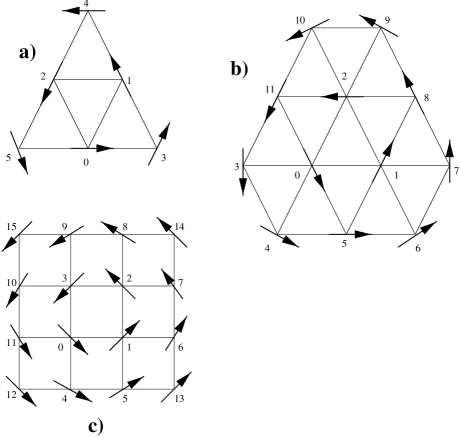
Figure 1: Classical vortex structrures on lattice samples which have a rotational symmetry axis intersecting the center of the vortex

Figure 2: Total square overlap of $|\psi_{+}\rangle$ in invariant subspaces of the Hamiltonian. The dashed line is a Gaussian with width $\Delta S^{z}$.

Figure 3: Square overlap of $|\psi_{\pm}\rangle$ with eigenstates of the Hamiltonian (upper diagram) and density of states as a function of the energy for the system of figure 1a) and $S=2$

Figure 4: Time evolution of local expectation values in the state $|\psi_{+}\rangle$ for the system of figure 1a) and $S=2$

Figure 5: Time evolution of local expectation values in the state $|\psi_{+}\rangle$ for the system of figure 1b) and $S=1/2$

Figure 6: The low–lying part of the spectrum of the system of figure 1a) for $S=2$

References

- [1] A. M. Kosevich, B. A. Ivanov, A. S. Kovalev, Phys. Rep. 194, 117 (1990)
- [2] M. E. Gouvea, G. M. Wysin, A. R. Bishop, F. G. Mertens, Phys. Rev. B 39, 11840 (1989)
- [3] F. G. Mertens, H. J. Schnitzer, A. R. Bishop, Phys. Rev. B 56, 2510 (1997)
- [4] S. Komineas, N. Papanicolaou, Nonlinearity 11, 265 (1998)
- [5] J. M. Kosterlitz, D. J. Thouless, J. Phys. C: Solid State Phys. 6, 1181 (1973), J. M. Kosterlitz, J. Phys. C: Solid State Phys. 7, 1046 (1974)
- [6] F. G. Mertens, A. R. Bishop, G. M. Wysin, C. Kawabata, Phys. Rev. B 39, 591 (1989)
- [7] J. E. R. Costa, B. V. Costa, D. P. Landau, Phys. Rev. B 57, 11510 (1998)
- [8] A. Cuccoli, V. Tognetti, P. Verrucchi, R. Vaia, Phys. Rev B 51, 12840 (1995)
- [9] J. Schliemann, F. G. Mertens, J. Phys.: Condens. Matter 10, 1091 (1998)
- [10] J. M. Radcliffe, J. Phys. A: Math. Gen. 4, 313 (1971)
- [11] V. S. Ostrovskii, Sov. Phys. JETP 64, 999 (1986)
- [12] B. A. Ivanov, A. N. Kichizhiev, D. D. Sheka, Sov. J. Low Temp. Phys. 18, 684 (1992)