Kinetics and thermodynamics across single-file pores: solute permeability and rectified osmosis

Abstract

We study the effects of solute interactions on osmotic transport through pores. By extending single-file, single-species kinetic models to include entrance of solute into membrane pores, we model the statistical mechanics of competitive transport of two species across membrane pores. The results have direct applications to water transport across biomembrane pores and particle movement in zeolites, and can be extended to study ion channel transport. Reflection coefficients, the reduction of osmotic fluxes measured using different solutes, are computed in terms of the microscopic kinetic parameters. We find that a reduction in solvent flow due to solute-pore interactions can be modelled by a Langmuir adsorption isotherm. Osmosis experiments are discussed and proposed. Special cases and Onsager relations are presented in the Appendices.

I Introduction

Recent X-ray[1] and electron crystallographic studies[2, 3] have yielded structures of integral membrane proteins such as K⁺ ion and water channels to near atomic resolution. Since many biological transport channels have specificity in allowing specific molecules to permeate and mediate simultaneous flows of numerous species.[4, 5] These new data may offer insights that may help correlate structure to function. The pores spanning biomembranes as well as those found in zeolites (important in numerous industrial processes such as hydrocarbon separations and catalytic agents) are typically few Angstroms in diameter, and contain very few molecules at any time. Therefore, we will study osmosis-driven particle transport across such pores using simple one-dimensional lattice models.

The next section reviews the linear phenomenological expressions[6] and their parameters, allowing for a second interacting, competing species. The empirical parameters arise from macroscopic considerations only and are not derived from any microscopic pore structure. Section III formally defines a two-species model similar to that used by Su et al.[7] and Wang et al.[8] Here, we assume a microscopic structure consisting of single-file pores. Unlike the single species case, where the statistics of one-dimensional particle dynamics are well understood,[9, 10, 11, 12, 13, 14] if solutes are allowed to enter a pore, no general analytical solution exists for the current across channels of arbitrary length. However, similar assumptions implicit in modelling single-species, single-file transport are used here: All nonlinearities except for those associated with the internal particle dynamics are neglected. Although our analysis is semiquantitative, and neglects some precise details about the specific particle-particle and particle-pore interactions, it provides a physically and mathematically consistent microscopic picture of nonequilibrium flow through single-file, solute permeable pores.

In the Solutions and Discussion section, we plot the behavior of steady state flows under a variety of experimentally motivated conditions. Certain macroscopic conjectures of the role of solute size on osmotic permeability[15] are re-examined. For short pores that allow partial and total passage of solute, the effective reflection coefficients (defined in Section II) and counterflow of solute are also computed and plotted in a number of illustrative graphs. An extension to longer pores is derived using an equilibrium multi-site Langmuir adsorption model.[16]

In the Conclusions, we summarize our analyses and discuss interpretations of osmosis measurements. We argue that models which intuitively incorporate solute-membrane interactions into linear coefficients[15] are inconsistent with a virial expansion in the solute-pore interactions. Possible experiments and correlations among the rate parameters are proposed. For completeness, the lattice statistics, rate equations for two-sectioned pores, Onsagers relations, and analytic solutions in a special case are treated in detail in the Appendices.

II Phenomenological Equations

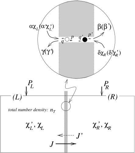
FIG. 1.: Schematic of osmosis and pressure driven flow through a membrane pore system. The reservoirs $(L)$ and $(R)$ are assumed infinite. The coefficients in the inset $\{\xi\}=(\alpha,\beta,\gamma,\delta,p,q)$, and $\{\xi^{\prime}\}=(\alpha^{\prime},\beta^{\prime},\gamma^{\prime},\delta^{\prime},p^{\prime},q^{\prime})$ are microscopic conditional transport rates for solvent and solute respectively and are defined by the figure. The solvent(solute) mole fractions in the $(L)$ and $(R)$ reservoirs are $\chi_{L}(\chi^{\prime}_{L})$ and $\chi_{R}(\chi^{\prime}_{R})$ respectively, and $\chi_{L,R}+\chi^{\prime}_{L,R}=1$. In a typical osmosis experiment, the membrane is impermeable to solute, (e.g. $\gamma^{\prime}$ or $\delta^{\prime}=0$), and the hydrostatic pressure difference $\Delta P=P_{R}-P_{L}=0$.

We first review the linear phenomenological equations describing two species transport across a membrane separating two infinite reservoirs (Fig. 1). When a membrane is permeable to solute as well as solvent, their fluxes, $J^{\prime}$ and $J$, are coupled. Following Katchalsky and Curran [6] and defining the fluxes in terms of a volume flow $J_{V}\equiv\tilde{v}J+\tilde{v}^{\prime}J^{\prime}$ conjugate to hydraulic pressure driving forces, and a relative flow $J_{D}\equiv J^{\prime}/n^{\prime}_{L}-J/n_{L}$ conjugate to diffusive driving forces, a set of linear Onsager relations are derived:

$$\begin{array}[]{ll}J_{V}&=L_{P}\Delta P+L_{PD}\Delta\Pi\\[13.0pt] J_{D}&=L_{DP}\Delta P+L_{D}\Delta\Pi.\end{array}$$ (1)

Here, $\tilde{v}(\tilde{v}^{\prime})$ is the molecular volume of solvent(solute) in solution, $n_{L}(n^{\prime}_{L})$ is the solvent(solute) particle number density in reservoir $(L)$. The osmotic pressure $\Delta\Pi\cong n_{T}k_{B}T\Delta\chi^{\prime}$, where $n_{T}$ is the total particle number density which we approximate as equal in the two reservoirs. The condition for zero volume flow $(J_{V}=0)$ requires $\Delta P=-(L_{PD}/L_{P})\Delta\Pi$. Thus, equilibrium across solute-impermeable membranes requires $\Delta P=\Delta\Pi$, and the reflection coefficient [6] $\Sigma\equiv-L_{PD}/L_{P}=1$. For permeable solutes, the condition for zero volume flow yields a reflection coefficient $\Sigma<1$ implying that a smaller hydraulic pressure is required to balance volume flow under a steady state osmotic pressure $\Delta\Pi$,

$$J_{V}=L_{P}(\Delta P-\Sigma\Delta\Pi).$$ (2)

Since $L_{PD}=-L_{P}\,(\Sigma=1)$ for an impermeable solute, $\Sigma$ can be measured by comparing $J_{V}$ induced by permeable solutes to the maximum ($J_{V}\equiv\tilde{v}J_{max}$) induced by impermeable solutes. However, the experimental measurement of

$$\Sigma={J_{V}\over\tilde{v}J_{max}}={\tilde{v}J+\tilde{v}^{\prime}J^{\prime}\over\tilde{v}J_{max}}$$ (3)

(under isobaric $\Delta P=0$ conditions) does not rely on the linearity assumed by (1), and nonlinear mechanisms may manifest themselves in $\Sigma$. Furthermore, as we will see, the current derived from an impermeable solute can also depend (to higher order in solute concentration difference $\Delta\chi^{\prime}$) on how the solute particles partly enter and bind to the pore interiors. Thus, measurements of $\Sigma$ may have more intricate dependences on solute-pore structure than is sometimes taken into account.

III Two Species 1D Exclusion Model

We now study flow mediated by one-dimensional channels. Single species exclusion models[9, 12, 13, 14] are extended to allow partial or complete entrance of solute particles inside a pore. This approach qualitatively models noncylindrical shapes[17] often found in biological pores and ion channels, i.e. flares, conical sections [1, 4], and vestibules [2] in the pore structure. These wider sections may allow solute entrance and binding, and may render the pore permeable to solute. Ion specific channels are also believed to have a narrower section near the midplane which acts like a selectivity filter for only those ions which can bind or pass through.

The one-dimensional chain shown in Fig. 1 which allows two types of particles (e.g. solvent and solute, or A and B) to enter and occupy any site.[10, 14] The kinetic rates pictured in Fig. 1 are defined as follows. A solvent particle enters site $i=1$ from $(L)$ with probability per unit time $dt$ or rate $\alpha\chi_{L}$ if and only if site $i=1$ is empty. This entrance rate is given by an intrinsic rate $\alpha$ times the mole fraction of solute particles in $(L)$. Similarly, the entrance rate from $(R)$ into the empty site $i=N$ is given by $\delta\chi_{R}$. The exit rates from the pore to the reservoirs at site $i=1,N$ provided they are occupied are $\gamma,\beta$ respectively. In the pore interior, a solvent particle hops to the left with probability $q$ only if the site $i-1$ to the left is empty. transitions to an empty site to the right are denoted by $p$. If the particles do not experience pondermotive forces (electrostatic or gravitational forces) and are being transported across microscopic, uniform pores, $p\simeq q$. However,, in general, the pores need not be uniform, and pondermotive forces (such as electric fields acting on charged particles) may also exist such that $p\neq q$. Completely analogous rates are defined for the second type of particle, or solutes, by primed quantities. The chain length is $L=N\ell$, where $\ell$ is set by the size of the larger of the two types of particles. If $a$ and $a^{\prime}$ are the approximate molecular sizes of the solvent and solute molecules, $a\gtrsim a^{\prime}/2$, then each site can contain at most one particle of either type.

By considering transitions among all possible particle configurations, the kinetic steps defined by (A1) and (A2) in Appendix A can be written in terms of dynamical rate equations. When solutes cannot enter the pore ($\alpha^{\prime}=\delta^{\prime}=0$), the solvent current $J_{max}$ across symmetric pores ($p=q$) in the presence of noninteracting solutes (i.e. $\alpha^{\prime}=\beta^{\prime}=\gamma^{\prime}=\delta^{\prime}=p^{\prime}=q^{\prime}=0$) is exactly[12, 13]

$$J_{max}(N)={p(\alpha\chi_{L}\beta-\gamma\delta\chi_{R})\over(N-1)(\alpha\chi_{L}+\gamma)(\beta+\delta\chi_{R})+p(\alpha\chi_{L}+\beta+\gamma+\delta\chi_{R})}.$$ (4)

When the solute particles can enter the pore, no analytic expressions exist for $J$, $J^{\prime}$. However, for illustration, consider a membrane so thin that $N=1$, and only boundary entrance and exit rates are relevant. The single site within the membrane can be in only one of three possible states: empty ($P_{1}$), solvent filled ($P_{2}$), and solute filled ($P_{3}$). The probability fluxes are determined by the rate equations

$$\begin{array}[]{ll}\partial_{t}P_{1}&=-\left(\alpha\chi_{L}+\alpha^{\prime}\chi^{\prime}_{L}+\delta\chi_{R}+\delta^{\prime}\chi^{\prime}_{R}\right)P_{1}+(\beta+\gamma)P_{2}+(\beta^{\prime}+\gamma^{\prime})P_{3}\\[13.0pt] \partial_{t}P_{2}&=(\alpha\chi_{L}+\delta\chi_{R})P_{1}-(\beta+\gamma)P_{2}\\[13.0pt] \partial_{t}P_{3}&=(\alpha^{\prime}\chi_{L}^{\prime}+\delta^{\prime}\chi_{R}^{\prime})P_{1}-(\beta^{\prime}+\gamma^{\prime})P_{3}\end{array}$$ (5)

Upon imposing steady state ($\partial_{t}P_{i}=0$), and normalization ($P_{1}+P_{2}+P_{3}\equiv 1$), the averaged occupations $\langle\sigma\rangle,\,\langle\sigma^{\prime}\rangle$ can be found and used in $J(N=1)=\alpha\chi_{L}(1-\langle\sigma\rangle-\langle\sigma^{\prime}\rangle)-\gamma\langle\sigma\rangle$ to find the steady state solvent current

$$J(N=1)={(\alpha\chi_{L}\beta-\gamma\delta\chi_{R})(\beta^{\prime}+\gamma^{\prime})\over(\alpha\chi_{L}+\beta+\gamma+\delta\chi_{R})(\beta^{\prime}+\gamma^{\prime})+(\alpha^{\prime}\chi^{\prime}_{L}+\delta^{\prime}\chi^{\prime}_{R})(\beta+\gamma)},$$ (6)

The solute current $J^{\prime}$ is given by interchanging $\{\xi\}\equiv(\alpha,\beta,\gamma,\delta)\leftrightarrow\{\xi^{\prime}\}\equiv(\alpha^{\prime},\beta^{\prime},\gamma^{\prime},\delta^{\prime})$ and $\chi_{L,R}\leftrightarrow\chi^{\prime}_{L,R}$ in (6). Note that $J(N=1)$ has the same form as $J_{max}(N=1)$ appropriate for single-species transport except for an additional term in the denominator,

$${(\alpha^{\prime}\chi^{\prime}_{L}+\delta^{\prime}\chi^{\prime}_{R})(\beta+\gamma)\over\beta^{\prime}+\gamma^{\prime}},$$ (7)

representing interference from states with solute occupation, $\sigma^{\prime}=1,(P_{3})$. The reflection coefficient defined for a single-site pore is thus

$$\begin{array}[]{l}\displaystyle\Sigma(N=1)=\displaystyle{1\over 1+{(\alpha^{\prime}\chi^{\prime}_{L}+\delta^{\prime}\chi^{\prime}_{R})(\beta+\gamma)\over(\alpha\chi_{L}+\beta+\gamma+\delta\chi_{R})(\beta^{\prime}+\gamma^{\prime})}}+{\tilde{v}\over\tilde{v}^{\prime}}{J^{\prime}(N=1)\over J_{max}(N=1)}\end{array}$$ (8)

and represents two factors; reduction of solvent flow (first term), and solute backflow (second term).

The microscopic activation energies $E_{\xi}(E^{\prime}_{\xi}),$ and the rate parameters $\{\xi\}=(\alpha,\beta,\gamma,\delta,p,q)$ and $\{\xi^{\prime}\}=(\alpha^{\prime},\beta^{\prime},\gamma^{\prime},\delta^{\prime},p^{\prime},q^{\prime})$, are governed by the microscopic membrane-solvent(solute) interactions, and are approximated by the Arrenhius forms $\xi\simeq\xi_{0}\exp(-E_{\xi}/k_{B}T)$ and $\xi^{\prime}\simeq\xi_{0}^{\prime}\exp(-E^{\prime}_{\xi}/k_{B}T)$.

Kinetic equations can be readily solved for slightly longer pores. The states and transition probabilities for a two species, two section ($N=2$) pore are enumerated in Appendix B. Currents across longer pores become increasingly tedious to compute as the matrix size increases as $3^{N}\times 3^{N}$. The general transition rates for an $N=3$ ($27\times 27$ matrix) pore are shown in Fig. 2 and will serve as the basis for most our subsequent analyses.

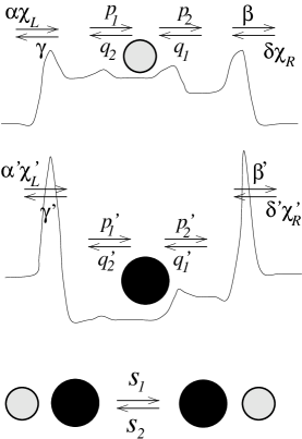
FIG. 2.: Schematic of a three sectioned pore displaying all microscopic energies and transition rates. Separate energy landscapes and occur for solvent(open circles) and solutes(filled circles). Exchange rates associated with wider pores are designated $s_{1},_{2}$. We take $s_{1}=s_{2}=s$ for the same reasons $q=p$.

IV Solutions and Discussion

Various effects of physical and chemical parameters, such as pore length and solute interaction dependences, are considered. We do not attempt to assign precise values to $\{\xi\},\{\xi^{\prime}\}$, but take the simplest, physically reasonable values to illustrate the relevant physical mechanisms.

A Solute Interacting, Impermeable Pores

First consider solutes only in the $(R)$-reservoir that can interact (i.e. partially enter) with a single-site ($N=1$) pore, but that encounters an infinite barrier while on the left side of the site (e.g. $\delta^{\prime}\neq 0,\gamma^{\prime}=\chi^{\prime}_{L}=0$). Assume for simplicity a pore that remains microscopically symmetric with respect interactions with the solvent. A reduction of solvent flux manifests itself in the definition of $\Sigma$ even though the pore is impermeable to solute and $J^{\prime}=0$. Thus $\Sigma(N=1,J^{\prime}=0)$ reduces to

$$\begin{array}[]{l}\displaystyle\Sigma_{\em eff}(N=1)\equiv{J(N=1)\over J_{max}(N=1)}\\[13.0pt] \displaystyle\>\quad\quad=\left[1+{2\delta^{\prime}\chi^{\prime}_{R}\over(2(\bar{\alpha}+1)-\bar{\alpha}\chi^{\prime}_{R})\beta^{\prime}}\right]^{-1}<1\end{array}$$ (9)

where $\bar{\alpha}\equiv\alpha/\beta$ defines an effective solvent-pore binding affinity.[18] We find the reduction in osmotic solvent flux for solutes that enter the site, represented by $\Sigma_{\em eff}$, depends mainly on the solute equilibrium constant $\delta^{\prime}\chi^{\prime}_{R}/\beta^{\prime}$, and $(\bar{\alpha}+1)^{-1}$. Since occupation of the site by solute is required to influence (block) solvent flow, the $\delta^{\prime}\chi^{\prime}_{R}/\beta^{\prime}$ behavior is not surprising. A low solvent affinity $\bar{\alpha}$ further allows the site to be more likely occupied by solute. These competitive factors determine the likelihood solute enters the pore and hinders solvent flux. Note that $\Sigma_{\em eff}(\chi^{\prime}_{R}\rightarrow 0)\rightarrow 1$.

The dependence on solute concentration $\chi^{\prime}_{R}$ is not unexpected. Qualitatively, one power of $\chi^{\prime}_{R}$ contributes the first order driving force for osmosis (the entropy of mixing); solute-solute (which we do not consider) and solute-membrane interactions must come at higher orders of $\Delta\chi^{\prime}$ via a virial expansion. Theories that suggest partial solute entrance into the pores [15, 19] as a mechanism for reducing solvent flows require the presence of solute in the vicinity (adsorbed near) the pore mouth. The likelihood of this configuration will depend on the bulk solute concentration. Thus, these types of nonlinearities can be effectively built into a concentration dependent $P_{os}=P_{os}(\Delta\chi^{\prime})$.[20] In the $\Delta\chi^{\prime}\rightarrow 0$ limit, $P_{os}$ approaches a constant (that depends only on how solvent travels through the membrane pore). The lowest order term is independent of solute identity.

Equation (9) arises from a Langmuir adsorption isotherm[16] determining the statistical fraction of solute-free (thus solvent conducting) states:

$$\Sigma_{\em eff}\simeq 1-P_{eq}\{\sigma^{\prime}=1\}\simeq{1+\alpha\chi_{L}/\beta\over Z}$$ (10)

where $Z\propto 1+\alpha\chi_{L}/\beta+\delta^{\prime}\chi^{\prime}_{R}/\beta^{\prime}$ is the partition function incorporating the three distinguishable pore occupancy states of the entire pore-$(R)$ reservoir ensemble. Equation (9) is recovered from (10).

While a single occupancy pore may not be molecularly realistic, many of its qualitative physical characteristics remain relevant for longer, multi-occupation pores. We explicitly compute flows in two (Appendix B) and three sectioned pores by calculating the coupled $9\times 9$ and $27\times 27$ rate equations. For these longer pores, the reduction of $J_{V}<J_{max}$ due to decreased solvent flux will also depend on where along the pore the membrane first becomes impenetrable to solute.

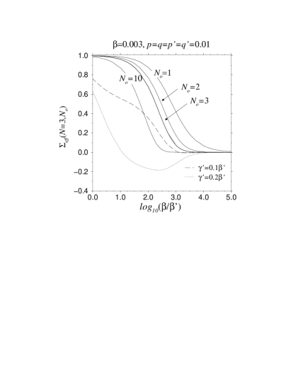
FIG. 3.: (a). Effective reflection coefficients $\Sigma_{\em eff}\equiv J(N=3)/J_{max}(N=3)$, as a function of solute-pore attraction $\beta^{\prime}$, for solute impermeable pores ($\gamma^{\prime}=0$, solid curves). The choice $\alpha=\delta=\delta^{\prime}=0.01,\beta=0.003$ corresponds to a slightly solvent attracting pore. The three sectioned pore allows solute entry into $N_{o}=1,2,\,\mbox{and}\,3$ of its sections, schematically shown in (b). Also shown by the broken curves are $\Sigma_{\em eff}$ (this does not include the volume transfer by backflow of solute, treated in Section III) when the solute is allowed to slowly permeate the pore, $(\gamma^{\prime}/\beta^{\prime}=0.1,0.2)$. The curve labelled $N_{o}=10$ is the equilibrium approximation (11) for a pore that allows solute entry into $\sim 10$ sites. Note the accuracy of (11) for $N_{o}=3$, which is nearly indistinguishable from the exact result. (b) Schematic of asymmetric pores allowing varying degrees of solute entrance.

Although solvent flux further decreases as solute is allowed to permeate deeper into the pore (allowing more solvent blocking configurations) solute-pore binding energies influence solute occupation exponentially. The sensitivity to solute-pore binding energy for various $N_{o}$ is demonstrated by Fig. 3(a), which shows the effective reflection coefficients for a three sectioned pore, $\Sigma_{\em eff}(N=3,N_{o})=J(N,N_{o})/J_{max}(N)$, as a function of the relative pore-solvent and pore-solute affinities. For concreteness we take $dt=10$fs, such that $(v_{T}/\ell)\sim 1$ps^-1 sets $p_{i}=q_{i}\simeq 0.01\ll 1$. Across pore sections that allow solute passage, we also assume $p^{\prime}=q^{\prime}=0.01$. These are reasonable estimates when considering molecular length, mass, and energy scales under ambient conditions. Sections that do not allow solute passage are defined by $p^{\prime}=0$ or $q^{\prime}=0$. The parameters used are $s=\alpha^{\prime}\chi^{\prime}_{L}=\gamma^{\prime}=0,\,\alpha=\delta=\delta^{\prime}=0.01$, and $\beta=0.003$. These values correspond to a slightly solvent-attracting pore ($\bar{\alpha}\simeq 3.33$), with identical intrinsic entrance rates for solvent or solute particles. The concentration $\chi^{\prime}_{R}=0.1/55.556$ corresponds to a 100mM aqueous solution in $(R)$. The measure of relative affinity $\log_{10}(\beta/\beta^{\prime})$ is varied by tuning the solute-pore attraction $\beta^{\prime}$ from $\alpha^{\prime}_{0}=0.01\rightarrow 0$. $N_{o}\leq N$ is the number of sections into the pore the solute can enter from $(R)$, as shown in Fig. 3(b). For example, when $N_{o}=2$, $p^{\prime}_{1}=p^{\prime}_{2}=q^{\prime}_{1}=0.01$ and $q^{\prime}_{2}=0$. The upper three solid curves in Fig. 3 represent the flux reduction from $J_{max}(N=3)$ due to solute entrance into one, two, and all three sites, corresponding to $q^{\prime}_{i}=0,q_{2}=0$, and $\gamma^{\prime}=0$ respectively.

The decrease of $\Sigma_{\em eff}$ for larger $N_{o}$ (the number of sites open or accessible to solute) can be physically understood in terms of a multisite Langmuir adsorption isotherm similar to that applied to the one-site model. The probability that there are no solute particles in any of the $N_{o}$ accessible sites is

$$\Sigma_{\em eff}(N,N_{o})\simeq\left[{1+\delta\chi_{R}/\beta\over 1+\delta\chi_{R}/\beta+\delta^{\prime}\chi^{\prime}_{R}/\beta^{\prime}}\right]^{N_{o}}.$$ (11)

This Increasing $N_{o}$, enhances the probability of nonconducting pores and can also be thought of as an additional entropic factor $k_{B}T\ln N_{o}$ in free energy difference favoring nonconducting (solute adsorbed pores) over conducting states. Equation (11) is valid provided $J$ is too small to significantly affect equilibrium occupancies. For the parameters used, the estimate (11) for $\Sigma(N_{o}=3)$ is nearly indistinguishable from the exact solution. The effective reflection coefficient (11) for $N\geq N_{o}=10$ ($\gamma^{\prime}=0,s=0$) is also indicated in Fig. 3. Note that the estimated relative flow reduction, (11), is independent of the total pore length $N$.

FIG. 4.: Solute concentration dependences of $\Sigma_{\em eff}$ are strongest highly attracting solute-pore species (small $\beta^{\prime}$). The $N$ dependence is negligible with under these parameters, consistent with the multisite Langmuir adsorption model (11).

Figure 4 shows the dependence of $\Sigma_{\em eff}(N,N_{o}=1)$ on solute concentration for $N=1,2,3$ at various solute bindings $\beta^{\prime}=0.00003,0.0003,0.003$. All other parameters are identical to those used in Fig. 3. The reflection coefficient decreases for larger solute concentration and smaller $\beta^{\prime}$ as expected. The independence of (11) on $N$ is also confirmed by the curves in Fig. 4, which are each three indistinguishable curves corresponding to $N=1,2,$ and 3.

B Solute Permeable Pores

When solute can steadily pass from $(R)$ to $(L)$ on time scales of the measurement,[21] the solute flow can nonnegligibly contribute to total volume flow. This flow comprises the solvent flux tending in one direction and solute flux tending in another. Therefore, the measured reflection coefficient $\Sigma$ (Eqn. (3)) can even be negative. The solvent current $J$ can also be independently negative, i.e. driven back by a strong counterflowing solute. Negative solvent flow is shown by the broken curves in Fig. 3 where the pore is permeable to solute ($\gamma^{\prime}>0$). The reflection coefficients measured and defined by $\Sigma_{\em eff}$ or (3) can thus be negative. However, for the $N=1$ case, we see from (6) that increasing $\gamma^{\prime}$ from zero can actually increase solvent flow $J$. This occurs particularly as $\chi^{\prime}_{L}\rightarrow 0$ and is the consequence of the additional route for emptying the solute from the membrane site to $(L)$, increasing the probability for a solute-free conducting state. This “backside” exiting effect will only occur for very short pores where a single kinetic step governed by $\gamma^{\prime}$ (in addition to $\beta^{\prime}$) renders the pore conducting and will disappear as $N$ increases.

The total volume flux, $J_{V}=\tilde{v}J+\tilde{v}^{\prime}J^{\prime}$ for $N=1$ found from (6) and $J^{\prime}$ can also increase as $\gamma^{\prime}$ increases provided $(\partial J_{V}/\partial\gamma^{\prime})>0$, which yields (for $\chi^{\prime}_{L}=0$,$\alpha=\delta$, and $\beta=\gamma$)

$${\beta\over\beta^{\prime}}>{2(\alpha+\beta)-\alpha\chi^{\prime}_{R}\over\alpha\chi^{\prime}_{R}(\tilde{v}/\tilde{v}^{\prime})-2\delta^{\prime}\chi^{\prime}_{R}}$$ (12)

Thus, a single site pore that is impermeable ($\gamma^{\prime}=0$) but allows solute entry only ($\delta^{\prime}\neq 0$) can actually increase net volume flow as it is made slightly permeable ($\gamma^{\prime}>0$). This anomalous behavior is more prevalent when $\tilde{v}^{\prime}/\tilde{v}$ and $\chi^{\prime}_{L}$ are small, since the volume backflow due to solute would be small and solute re-entrance rates from $(L)$ vanish.

FIG. 5.: Currents for various internal solute barrier heights occuring at different positions. $N_{o}=1,2,3$ correspond to $1,2,3$ easily solute-accessible sites within an $N=3$ pore. The quantity $x^{\prime}_{i}=q^{\prime}_{1},q^{\prime}_{2},\gamma^{\prime}$ measures the hopping rate to the left past this site.

In Fig. 5, we relax the impermeable solute constraint and allow for passage of solute from $(R)\rightarrow(L)$. Heights of the rate limiting internal barrier is varied relative to $\beta^{\prime}$ at various internal positions $i$, where $x^{\prime}_{i}=q^{\prime}_{1},q^{\prime}_{2}$, or $\gamma^{\prime}$. The $x^{\prime}_{i}/\beta^{\prime}\rightarrow 0$ limit of $J$ and $J^{\prime}$ approach those expected from simple osmosis resulting from an impermeable (although pore-entering) solute, as studied in Fig. 3. As impermeability is relaxed, $J$ decreases, while $J^{\prime}$ becomes negative. The effects are most pronounced for pores that have the largest number of easy entrance sites (e.g. $N_{o}=3$). In fact, for solute-binding pores where $q^{\prime}_{i}/\beta^{\prime}>1$, and larger $N$, the negative solute flux can actually drag, or pump solvent backwards ($N_{o}=3$ curves in (b). for $\gamma^{\prime}/\beta^{\prime}\gtrsim 1$).

FIG. 6.: (a). Solvent and solute fluxes as functions of relative pore-solute, pore-solvent binding affinity $\log(\alpha^{\prime}\beta/\alpha\beta^{\prime})$ (with $\alpha,\beta$ fixed). To the left of the discontinuity, (defined by $\alpha^{\prime}_{0}=0.003,\beta^{\prime}_{0}=0.01$ and most evident for $N=1$) the pore is solute-repelling, and $\alpha^{\prime}$ is being varied, while to the right, the pore is being made increasingly solute-attractive by decreasing $\beta^{\prime}$. (b). The associated total pore occupancies.

Negative solvent flux is shown in Fig. 6. Here, we assume a molecularly symmetric (with respect to both solvent and solute) pore such that $\beta^{\prime}=\gamma^{\prime},\beta=\gamma$ and $q=p$ is constant along the pore, as assumed in the specific dynamical model presented in Appendix A. Figure 6(a) shows the currents $J(N=3),J^{\prime}(N=3)$ as functions of the solute-pore affinity $\alpha^{\prime}/\beta^{\prime}$ expressed in terms of the logarithm of the relative (to solvent-pore binding fixed at $\alpha=0.01,\beta=0.003$) affinities. The discontinuity at $\log(\alpha^{\prime}_{0}/\beta^{\prime}_{0})=\log(0.003/0.01)$ indicates the crossover from solute-repelling to solute-attracting pores. Only at intermediate solute affinity, and longer pores ($N\geq 3$), does solute current $J^{\prime}<0$ sweep solvent in a direction opposite from that expected from simple osmosis. Pores that repel solute rarely contain such particles that drive solvent up its chemical potential gradient $\Delta\mu$. However, pores that bind strongly to solute are choked off, and both $J$ and $J^{\prime}$ diminish. Fig. 6(b) shows the associated total pore occupancies $\sum_{i}^{N}\langle\sigma_{i}\rangle$ and $\sum_{i}^{N}\langle\sigma^{\prime}_{i}\rangle$.

FIG. 7.: Solvent and solute fluxes across symmetric solute permeable pores as function of solute concentrations. (a) $\chi^{\prime}_{L}=0$ as $\Delta\chi^{\prime}=\chi^{\prime}_{R}$ is varied. The lower three thin curves and upper thick curves depict solute ($J^{\prime}<0$) and solvent flow respectively. The parameters used correspond to a solvent attracting pore with strong solute binding (solid curves), intermediate binding (dotted courves), and solute repelling (dashed curves) pores. (b) The currents as absolute concentration $\chi^{\prime}_{L}$ is varied, with $\Delta\chi^{\prime}=0.1/55.556$ fixed.

Figure 7(a) shows the dependences of $J(N=3)$ and $J^{\prime}(N=3)$ on solute concentration difference $\Delta\chi^{\prime}$ with $\chi^{\prime}_{L}=0$. For strong solute-binding pores (low $\beta^{\prime}$, solid curves), the solvent current $J(N=3)<0$ due to a strong solute backflow $J^{\prime}(N=3)<0$. In Fig 7(b), we vary $\chi^{\prime}_{L}$ while keeping $\Delta\chi^{\prime}=0.1/55.556$ fixed. The higher absolute solute concentrations in this case decrease solvent occupation allowing a larger current in the same direction as osmosis, and solute is swept in the same direction $J^{\prime}>0$. However, for too strong a solute binding, increasing solute occupation eventually clogs the pore, precluding efficient solvent flow (solid curves). Here, at low absolute concentrations, $J,J^{\prime}<0$ indicating that solute is pushing solvent back against the direction expected from simple osmosis.

FIG. 8.: Currents across a symmetric, $N=3$ pore as a function of $s_{1}=s_{2}=s$. Concentrations used are $\chi^{\prime}_{L}=0,\chi^{\prime}_{R}=0.1/55.556$.

Effects of “slip” $s_{1}=s_{2}=s$ (see Fig. 2) are explored in Fig. 8. The magnitudes of both $J(N=3)$ and $J^{\prime}(N=3)$ are increased as $s$ increases since the counterflowing currents are occasionally allowed to more easily pass through each other. This variation is strongest for smaller $\beta^{\prime}$ (strong solute-binding pore) since large solute occupation configurations would be most influenced by slip. Note the near symmetry between $J$ and $-J^{\prime}$ when $\beta=\beta^{\prime}=0.003$.

V Summary and Conclusions

We have studied a commonly measured figure of merit, the reflection coefficient $\Sigma$ (which describes the reduction in fluid volume transport in the presence of permeable or membrane interacting solutes). The single site model of Kalko et al.[22] is extended to include longer pores and the effects of solute penetration and binding. The currents and reflection coefficints (Figs. 3-8) were computed in terms of microscopic molecular parameters in some limiting, yet illustrative cases. Solutes that enter and bind to pore interiors block and reduce solvent flux without being completely permeable, yielding an effective reflection coefficient $\Sigma_{\em eff}<1$. Although higher order corrections to van’t Hoff’s law have been studied [16, 23] and is well understood in terms of virial expansions of solute-solute interactions in the reservoirs, solute fouling arises from higher order concentration terms resulting from solute-membrane/pore interactions. Although the phenomenological Onsager coefficients $L_{P},L_{PD}=L_{DP},L_{D}$ can be qualitatively approximated from our plots of $J$ and $J^{\prime}$, care must be exercised when interpreting measurements since solute interference effects can be highly nonlinear, when Eqns. 1 do not apply. The magnitudes of the nonlinear effects depend on solute-pore interaction energies as well as the number of configurations that are solvent blocking, both of which can be inferred from microscopic models of the particular pore-solute system being considered.

For a one-site pore that allows solute entrance but remains solute-impermeable “solute interference” nonetheless reduces the solvent flux $J$ by a factor $\propto\chi^{\prime}_{R}\exp\left[(-E^{\prime}_{\delta^{\prime}}+E^{\prime}_{\beta})/k_{B}T\right]$, where $\chi^{\prime}_{R}$ is the solute mole fraction, and $E^{\prime}_{\delta}$ and $E^{\prime}_{\beta}$ are the solute-pore “in” and “out” energetic barriers. Because the nonlinearities are most pronounced for large $\delta^{\prime}/\beta^{\prime}$, e.g. a very large $E^{\prime}_{\beta}$ or a highly solute-binding pore, strong solute binding leads to the most effective solvent flow reduction. Measurements of $J$ vs. $\chi^{\prime}_{R}$ with different solutes should have the same slope as $\chi^{\prime}_{R}\rightarrow 0$. If different solutes can indeed yield different slopes,[24] the interactions are too strong for the linear limit to have been reached. Extreme cases are “solutes” such as mercurial compounds $p$-chloromecuribenzoate (PCMB) that can reversibly destroy aquaporin pore function at very low concentrations[25] due to strong binding; although here, the binding is so strong that pore structure is presumably altered. Experimentally, the solute concentration dependence on reflection coefficients has been observed in various systems.[19, 20, 26]

One possible experiment to probe solute blockage effects in asymmetric (with respect to solutes) pores and flow rectification[19] is to compare the currents $J$ and $-J$ associated with solutes in the $(L)$ and $(R)$ reservoirs. For a symmetric pore, the magnitudes of the currents will be equal. However, for asymmetric pores, flow induced by solutes in $(L)$ will be different from that generated by solutes in $(R)$, the difference being manifested in higher order terms in solute concentration.

If the pore is permeable to solute $(J^{\prime}\neq 0)$, and $\Sigma$ is defined by measuring the total volume flux $J_{V}=\tilde{v}J+\tilde{v}^{\prime}J^{\prime}$, a negative reflection coefficient $\Sigma<0$ can even occur when the counterflowing solute adds to a possibly counterflowing solvent, or overcompensates for the co-flowing solvent. For solute-permeable pores, correlations between volume flow and solute size typically used in macroscopic descriptions, when extended to the microscopic regime considered here, are not straightforward since $J_{V}$ depends directly on $\tilde{v}^{\prime}$ as well as on the rate parameters $\{\xi^{\prime}\}$. The notion of molecular size alone, based on van der Waal’s radii for example, neglects pore-particle attractions and nonadditive interactions among molecules such as hydrogen bonding. For example, urea may easily enter pores based on its small size (and thus have a larger $N_{o}$), but participates in strong H-bonding in aqueous solution, implying a very small $\alpha^{\prime}/\beta^{\prime}$ (solute-repelling pore) since H-bonds need to be broken prior to pore entry. Urea might then be expected to yield a larger measured reflection coefficient than that expected from its molecular size alone.[27] H-bonding in the bulk solution may also significantly change $D^{\prime}$ and affect the interpretation if unstirred layers are important. Furthermore, the additional solute interactions giving rise to $\Sigma_{\em eff},\Sigma$ provide additional energy scales which can yield apparently non-Arrhenius temperature dependences.[28]

The treatment given suggests that correlations between thermodynamic solute-solvent parameters and pressure or osmosis driven flows can be partly experimentally determined. Specific volume changes of bulk solute-solvent mixing, and enthalpies of mixing determine $\tilde{v}^{\prime}/\tilde{v}$ and constrains $\{\xi,\xi^{\prime}\}$. For example, a solute with a negative enthalpy of mixing (with solvent), $\Delta H_{m}$, would have a smaller $\delta^{\prime}/\beta^{\prime}$ than a solute-solvent pair with larger or positive $\Delta H_{m}$. Equilibrium measurements of relative solvent and solute absorption in pores also give relative measures of the parameters $\delta^{\prime}/\beta^{\prime}$ and $\alpha/\beta$. Further refinement of the parameters $\{\xi\},\,\{\xi^{\prime}\}$ may be obtained with more precise molecular mechanics [29] or molecular dynamics dynamics (MD) using appropriate molecular force fields.[22] Direct MD simulation of osmosis across very thin membrane pores (single atomic layers) have even been performed for high solute concentrations.[30] Nonequilibrium MD simulations have also been used to compute dynamic separation factors for two species flows.[31] Monte-Carlo simulations may also reveal qualitatively interesting behavior in transport across longer channels.

A 1D chain dynamics

For arbitrarily long pores, the dynamical rules of particle transport incorporating exclusion interactions can be formally implemented on a discrete lattice. If $\sigma_{i}(\sigma_{i}^{\prime})\in\{0,1\}$ denote the solvent(solute) particle occupation at site $i$, the instantaneous rules for the microscopic transport of the two species in the pore interior are mathematically defined by

$$\begin{array}[]{rl}J_{i,i+1}&=\hat{p}\sigma_{i}(1-\sigma_{i+1})(1-\sigma^{\prime}_{i+1})-\hat{q}\sigma_{i+1}(1-\sigma_{i})(1-\sigma^{\prime}_{i})\\[13.0pt] J^{\prime}_{i,i+1}&=\hat{p}^{\prime}\sigma^{\prime}_{i}(1-\sigma_{i+1})(1-\sigma^{\prime}_{i+1})-\hat{q}^{\prime}\sigma^{\prime}_{i+1}(1-\sigma_{i})(1-\sigma^{\prime}_{i})\end{array}$$ (A1)

where $(\hat{p},\hat{q},\hat{p}^{\prime},\hat{q}^{\prime})\in(0,1)$. The time variable has been suppressed for notational simplicity. These rules incorporate excluded volume into the dynamics of both solvent and solute. Equations (A1) are supplemented with the boundary transition rates

$$\begin{array}[]{rl}J_{(L),1}&=\hat{\alpha}(1-\sigma_{1})(1-\sigma^{\prime}_{1})-\hat{\gamma}\sigma_{1}\\[13.0pt] J_{N,(R)}&=\hat{\beta}\sigma_{N}-\hat{\delta}(1-\sigma_{N})(1-\sigma^{\prime}_{N})\\[13.0pt] J^{\prime}_{(L),1}&=\hat{\alpha}^{\prime}(1-\sigma_{1})(1-\sigma^{\prime}_{1})-\hat{\gamma}^{\prime}\sigma^{\prime}_{1}\\[13.0pt] J^{\prime}_{N,(R)}&=\hat{\beta}^{\prime}\sigma^{\prime}_{N}-\hat{\delta}^{\prime}(1-\sigma_{N})(1-\sigma^{\prime}_{N})\end{array}$$ (A2)

Upon taking the time or ensemble average of the above equations, and assuming the rate parameters are independent of the dynamical variables $\sigma,\sigma^{\prime}$, we formally obtain steady state flows that depend on $\{\xi,\xi^{\prime}\}$, the $dt\rightarrow 0$ limit of the averages of $\{\hat{\xi},\hat{\xi}^{\prime}\}$. However, the time averaged currents are not easily solved due to higher order correlations among $\sigma,\sigma^{\prime}$ such as $\langle\sigma_{i+1}\sigma^{\prime}_{i}\rangle$, etc.[10, 14] Nonetheless, transport across very short (small $N$) pores can be solved using rate equations defined by the rates $\{\xi\},\{\xi^{\prime}\}$ found from the mean of the distribution of $\{\xi\},\{\xi^{\prime}\}\in\{0,1\}$.

B Two Species Two Site model

Consider a membrane thick enough to accommodate a pore that can simultaneously fit two particles, solvent or solute, along its axis. We assume that the particle-particle interactions are dominated by excluded volume effects such that longer ranged microscopic interactions that cooperatively affect the particle hopping rates can be neglected. At any instant, either of the two partitions in the pore must be in one of three occupation states, empty, solvent(open circle), or solute(filled circle). Therefore, there are $3\times 3=9$ microscopic states denoted by

$$\begin{array}[]{llllll}&&P_{1}&&{}^{\mbox{\circle*{13.0}}}&P_{5}\\[13.0pt] \bigcirc&&P_{2}&{}^{\mbox{\circle*{13.0}}}&&P_{6}\\[13.0pt] &\bigcirc&P_{3}&\!\!\!\bigcirc&{}^{\mbox{\circle*{13.0}}}&P_{7}\\[13.0pt] \bigcirc&\bigcirc&P_{4}&{}^{\mbox{\circle*{13.0}}}&\!\!\!\bigcirc&P_{8}\\[13.0pt] &&&{}^{\mbox{\circle*{13.0}}}&{}^{\mbox{\circle*{13.0}}}&P_{9}\end{array}$$ (B1)

where the transitions among the probabilities are given by the coupled rate equations

$$\partial_{t}P_{i}+A_{ij}P_{j}=0$$ (B2)

with the transition matrix defined by ${\bf A}=$

$$\!\!\!\!\!\!\!\!\!\!\!\!\!\!\left(\begin{array}[]{ccccccccc}\alpha_{T}+\delta_{T}&-\gamma&-\beta&0&-\gamma^{\prime}&-\beta^{\prime}&0&0&0\\ -\alpha\chi_{L}&\gamma+\delta_{T}+q&-p&-\beta&0&0&0&-\beta^{\prime}&0\\ -\delta\chi_{R}&-q&\alpha_{T}+\beta+p&-\gamma&0&0&-\gamma^{\prime}&0&0\\ 0&-\delta\chi_{R}&-\alpha\chi_{L}&\gamma+\beta&0&0&0&0&0\\ -\alpha^{\prime}\chi^{\prime}_{L}&0&0&0&\delta_{T}+\gamma^{\prime}+q^{\prime}&-p^{\prime}&-\beta&0&-\beta^{\prime}\\ -\delta^{\prime}\chi^{\prime}_{R}&0&0&0&-q^{\prime}&\alpha_{T}+\beta^{\prime}+p^{\prime}&0&-\gamma&-\gamma^{\prime}\\ 0&0&-\alpha^{\prime}\chi^{\prime}_{L}&0&-\delta\chi_{R}&0&\gamma^{\prime}+\beta+s^{\prime}&-s&0\\ 0&-\delta^{\prime}\chi^{\prime}_{R}&0&0&0&-\alpha\chi_{L}&-s^{\prime}&+\gamma+\beta^{\prime}+s&0\\ 0&0&0&0&-\delta^{\prime}\chi^{\prime}_{R}&-\alpha^{\prime}\chi^{\prime}_{L}&0&0&\beta^{\prime}+\gamma^{\prime}\end{array}\right)$$ (B3)

where $\alpha_{T}(\delta_{T})\equiv\alpha\chi_{L}+\alpha^{\prime}\chi^{\prime}_{L}(\delta\chi_{R}+\delta^{\prime}\chi^{\prime}_{R})$. The coefficients are defined by the elementary steps shown in Figure 1; $\alpha,\beta,\gamma,\delta$ and their primed analogues carry the same physical meaning as in the one site model. The quantities $q(p),q^{\prime}(p^{\prime})$, and $s(s^{\prime})$ define the microscopic rates of transitions $P_{2}\rightarrow P_{3}(P_{3}\rightarrow P_{2})$, $P_{5}\rightarrow P_{6}(P_{6}\rightarrow P_{5})$, and $P_{8}\rightarrow P_{7}(P_{7}\rightarrow P_{8})$, respectively. Probability distributions $P_{i}$ are found by solving Eq. (B2) with (B3) and the constraint $\sum_{i=1}^{9}P_{i}=1$. Form these, the steady state solvent and solute currents are

$$\begin{array}[]{rl}J&=\alpha\chi_{L}(P_{1}+P_{3}+P_{6})-\gamma(P_{2}+P_{4}+P_{8})\\[13.0pt] J^{\prime}&=\alpha^{\prime}\chi^{\prime}_{L}(P_{2}+P_{3}+P_{6})-\gamma^{\prime}(P_{5}+P_{7}+P_{9}).\end{array}$$ (B4)

An analogous set of equations hold for the kinetics of a three section, two-species pore.

C $N$ site, Two-Species Case

We generalize the single section model to $N$ sections. Under special cases, analytic expressions can be found for general $N$. Using notation describing the one section, the time averaged fluxes of $\sigma$ and $\sigma^{\prime}$ particles are

$$\begin{array}[]{l}J=p\langle\sigma_{i}-\sigma_{i+1}\rangle+(p-s)\langle\sigma_{i+1}\sigma^{\prime}_{i}-\sigma_{i}\sigma^{\prime}_{i+1}\rangle\\[13.0pt] J^{\prime}=p^{\prime}\langle\sigma^{\prime}_{i}-\sigma^{\prime}_{i+1}\rangle+(p^{\prime}-s)\langle\sigma_{i}\sigma^{\prime}_{i+1}-\sigma_{i+1}\sigma^{\prime}_{i}\rangle,\end{array}$$ (C1)

since $\langle\sigma_{i}\sigma_{i}^{\prime}\ldots\rangle=0$. The steady state volume flux $J_{V}\equiv\tilde{v}J+\tilde{v}^{\prime}J^{\prime}$ in the interior and at the boundaries are

$$\begin{array}[]{l}J_{V,i}=\tilde{v}p\langle\sigma_{i}-\sigma_{i+1}\rangle+\tilde{v}^{\prime}p^{\prime}\langle\sigma_{i}^{\prime}-\sigma_{i+1}^{\prime}\rangle+\left[(p-s)\tilde{v}-(p^{\prime}-s)\tilde{v}^{\prime}\right]\langle\sigma_{i+1}\sigma_{i}^{\prime}-\sigma_{i}\sigma_{i+1}^{\prime}\rangle\\[13.0pt] J_{V,1}=(\tilde{v}\alpha\chi_{L}+\tilde{v}^{\prime}\alpha^{\prime}\chi^{\prime}_{L})-Q_{L}\langle\sigma_{1}\rangle-Q^{\prime}_{L}\langle\sigma^{\prime}_{1}\rangle\\[13.0pt] J_{V,N}=-(\tilde{v}\delta\chi_{R}+\tilde{v}^{\prime}\delta^{\prime}\chi^{\prime}_{R})+Q_{R}\langle\sigma_{N}\rangle+Q^{\prime}_{R}\langle\sigma^{\prime}_{N}\rangle.\end{array}$$ (C2)

where

$$\begin{array}[]{rl}Q_{L}&=\tilde{v}\alpha\chi_{L}+\tilde{v}^{\prime}\alpha^{\prime}\chi^{\prime}_{L}+\tilde{v}\gamma\\[13.0pt] Q^{\prime}_{L}&=\tilde{v}\alpha\chi_{L}+\tilde{v}^{\prime}\alpha^{\prime}\chi^{\prime}_{L}+\tilde{v}^{\prime}\gamma^{\prime}\\[13.0pt] Q_{R}&=\tilde{v}\delta\chi_{R}+\tilde{v}^{\prime}\delta^{\prime}\chi^{\prime}_{R}+\tilde{v}\beta\\[13.0pt] Q^{\prime}_{R}&=\tilde{v}\delta\chi_{R}+\tilde{v}^{\prime}\delta^{\prime}\chi^{\prime}_{R}+\tilde{v}^{\prime}\beta^{\prime}.\end{array}$$ (C3)

The quadratic terms in $J_{V,i}$ cancel provided

$$(p-s)\tilde{v}=(p^{\prime}-s)\tilde{v}^{\prime}.$$ (C4)

Under this special condition, it is useful to define $\sigma^{+}_{i}\equiv p\tilde{v}\sigma_{i}+p^{\prime}\tilde{v}^{\prime}\sigma^{\prime}_{i}$ so that the current can be summed as

$$J_{V}={\langle\sigma^{+}_{1}-\sigma^{+}_{N}\rangle\over N-1}.$$ (C5)

The volume flux $J_{V}$ is completely determined when the boundary currents depend only upon $\sigma^{+}$, which is the case provided

$${Q_{L}\over Q^{\prime}_{L}}={Q_{R}\over Q^{\prime}_{R}}={\tilde{v}p\over\tilde{v}^{\prime}p^{\prime}}.$$ (C6)

The above relationships, along with (C4) provide constraints among $\alpha^{\prime},\,\beta^{\prime},\,\gamma^{\prime},\,\delta^{\prime}$ given $\alpha,\,\beta,\,\gamma,\,\delta$. In the simple case of no-pass pores, $s=0$, a simple scaling exists;

$$p^{\prime}=p\phi,\quad\beta^{\prime}=\beta\phi,\quad\gamma^{\prime}=\gamma\phi$$ (C7)

where $\phi\equiv\tilde{v}/\tilde{v}^{\prime}$. These special conditions imply larger (in the aqueous bulk phase) solute are more sluggish in hopping between sections and into and out of the pore, and are not qualitatively unreasonable. In this illustrative case, the volume flux is

$$J_{V}(N)={\gamma(\tilde{v}\delta-\tilde{v}^{\prime}\delta^{\prime})\Delta\chi^{\prime}+\tilde{v}(\alpha\beta-\gamma\delta)\chi^{\prime}_{L}+\tilde{v}^{\prime}(\alpha^{\prime}\beta-\gamma\delta^{\prime})\chi^{\prime}_{L}\over(N-1)Q_{L}Q_{R}+p\tilde{v}(Q_{L}+Q_{R})},$$ (C8)

an implicit function of $\Delta P$. In the $\chi^{\prime}_{L}=0$, isobaric ($\Delta P\propto\alpha\beta-\gamma\delta=0$) limit the sign of $J^{\prime}$ is determined by $\tilde{v}\delta-\tilde{v}^{\prime}\delta^{\prime}$.

D Onsager relations for one site model

We have only explicitly considered osmotic flow between isobaric reservoirs $(L)$ and $(R)$. However, when a hydraulic pressure is applied, the enthalpies between the two baths will generally be unequal, and two independent thermodynamic driving forces may exist. For microscopically symmetric pores ($\alpha=\delta,\alpha^{\prime}=\delta^{\prime}$), the differences $\Delta E$ and $\Delta E^{\prime}$ can be readily related to hydrostatic pressure differences. Expanding the solutions (6) and $J^{\prime}(N=1)$ about $\Delta\chi^{\prime}=0$ and $P_{L}=P_{R}$, we find

$$\begin{array}[]{rl}J&=P_{os}\Delta\Pi-L_{p}\Delta P\\[13.0pt] J^{\prime}&=-P^{\prime}_{os}\Delta\Pi-L^{\prime}_{p}\Delta P\end{array}$$ (D1)

where the coefficients in terms of the microscopic kinetic parameters are

$$\begin{array}[]{rl}\displaystyle P_{os}&\displaystyle={\alpha\gamma\gamma^{\prime}\over 2n_{T}k_{B}T(\alpha\gamma^{\prime}\chi_{L}+\alpha^{\prime}\gamma\chi^{\prime}_{L}+\gamma\gamma^{\prime})}\\[13.0pt] \displaystyle P^{\prime}_{os}&\displaystyle={\alpha^{\prime}\gamma\gamma^{\prime}\over 2n_{T}k_{B}T(\alpha\gamma^{\prime}\chi_{L}+\alpha^{\prime}\gamma\chi^{\prime}_{L}+\gamma\gamma^{\prime})}\\[13.0pt] \displaystyle L_{p}&\displaystyle={\alpha\gamma\gamma^{\prime}\chi_{L}\tilde{v}\over 2k_{B}T(\alpha\gamma^{\prime}\chi_{L}+\alpha^{\prime}\gamma\chi^{\prime}_{L}+\gamma\gamma^{\prime})}\\[13.0pt] \displaystyle L^{\prime}_{p}&\displaystyle={\alpha^{\prime}\gamma\gamma^{\prime}\chi^{\prime}_{L}\tilde{v}^{\prime}\over 2k_{B}T(\alpha\gamma^{\prime}\chi_{L}+\alpha^{\prime}\gamma\chi^{\prime}_{L}+\gamma\gamma^{\prime})},\end{array}$$ (D2)

where we have assumed an attractive pore and linearized the exit rates using their Arrhenius forms according to

$$\beta\simeq\gamma+\left({\partial\beta\over\partial P_{R}}\right)_{P_{R}=P_{L}}\!\!\!\!\Delta P=\gamma-{\gamma\over k_{B}T}\left({\partial E_{\beta}\over\partial P_{R}}\right)\Delta P,$$ (D3)

and the Maxwell relation $(\partial E_{\beta}/\partial P_{R})=\tilde{v}$.

Upon forming the conjugate flows and using the definition (1),

$$\begin{array}[]{rl}\displaystyle L_{P}&\displaystyle=-{\alpha\gamma\gamma^{\prime}\chi_{L}\tilde{v}^{2}+\alpha^{\prime}\gamma\gamma^{\prime}\chi^{\prime}_{L}\tilde{v}^{\prime 2}\over 2k_{B}T(\alpha\gamma^{\prime}\chi_{L}+\alpha^{\prime}\gamma\chi^{\prime}_{L}+\gamma\gamma^{\prime})}\\[13.0pt] \displaystyle L_{PD}=L_{DP}&\displaystyle={\alpha\gamma\gamma^{\prime}\tilde{v}-\alpha^{\prime}\gamma\gamma^{\prime}\tilde{v}^{\prime}\over 2n_{T}k_{B}T(\alpha\gamma^{\prime}\chi_{L}+\alpha^{\prime}\gamma\chi^{\prime}_{L}+\gamma\gamma^{\prime})}\\[13.0pt] \displaystyle L_{D}&\displaystyle={\alpha\gamma\gamma^{\prime}\chi_{L}-\alpha^{\prime}\gamma\gamma^{\prime}\chi^{\prime}_{L}\over 2n_{T}^{2}k_{B}T(\alpha\gamma^{\prime}\chi_{L}+\alpha^{\prime}\gamma\chi^{\prime}_{L}+\gamma\gamma^{\prime})}\end{array}$$ (D4)

which manifestly satisfies Onsager reciprocity. Corresponding expressions for longer pores are very cumbersome but can be evaluated with e.g. Mathematica.

REFERENCES

• [1] D. A. Doyle, J. M. Cabral, R. A. Pfuetzner, A. L. Kuo, J. M. Gulbis, S. L. Cohen, B. T. Chait, and R. MacKinnon, Science, 280, 69-77, (1998).
• [2] A. Cheng, A. N. van Hoek, M. Yeager, A. S. Verkmen, and A. K., and Mitra, Nature, 387, 627-630, (1997).
• [3] B. K. Jap and H. Li, J. Mol. Biol., 251, 413-420, (1995).
• [4] A. Finkelstein, Water Movement Through Lipid Bilayers, Pore, and Plasma Membranes, (Wiley-Interscience, New York, 1987).
• [5] T. Zeuthen, Int. Rev. Cytology, 160, 99, (1995).
• [6] A. Katchalsky, P. F. and Curran, Nonequilibrium Thermodynamics in Biophysics, (Harvard University Press, Cambridge, 1965)
• [7] A. Su, S. Mager, S. L. Mayo, and H. A. Lester, Biophys. J., 70, 762, (1996).
• [8] K.-W. Wang, S. Tripathi, and S. B. Hladky, J. Membr. Bio., 143, 247, (1995).
• [9] H. van Beijeren, K. W. Kehr, and R. Kutner, Phys. Rev. B, 28, 5711, (1983).
• [10] R. B. Stinchcombe and G. M. SchΓΌltz, Phys. Rev. Lett., 75, 140, (1995); Nonequilibrium Statistical Mechanics in One Dimension, Ed. V. Privman, (Cambridge University Press, 1997).
• [11] M. R. Evans, D. P. Foster, C. GodrΓ¨che, and D. Mukamel, J. Stat. Phys., 80, 69-102, (1995).
• [12] T. Chou, Phys. Rev. Lett., 80, 85-88, (1998).
• [13] T. Chou, To be published.
• [14] C. RΓΆdenbeck, J. KΓ€rger, and K. Hahn, Phys. Rev. E, 55(5), 5697-5712, (1997).
• [15] A. E. Hill, Int. Rev. Cytology, 163, 1-42, (1995).
• [16] T. L. Hill, An Introduction to Statistical Thermodynamics, (Dover, New York, 1986).
• [17] S. Sokolowski, Molecular Physics, 75(6), 1301, (1992).
• [18] Since $\alpha$ is an intrinsic entrance, or β€œon” rate, and $\beta$ is an β€œoff” rate, the ratio $\bar{\alpha}\equiv\alpha/\beta$ gives an effective equilibrium solvent-pore binding constant averaged across the pore.
• [19] C. J. Toupin, M. Le Maguer, and L. E. McGann, Cryobiology, 26, 431-444, (1989).
• [20] R. I. Sha’afi, G. T. Rich, D. C. Mikulecky, and A. K. Solomon, J. Gen. Physiol., 55, 427-450, (1970).
• [21] Strictly speaking, all membranes are solute permeable, given sufficient time for particle tunneling.
• [22] S. G. Kalko, J. A. Hernandez, Biochim. et Biophys. Acta-Biomembranes, 1240(2), 159, (1995).
• [23] J. A. Cohen and S. Highsmith, Biophys. J., 73, 1689, (1997); C. Reid and R. P. Rand, Biophys. J., 73, 1692, (1997).
• [24] A. E. Hill, Private Communication
• [25] C. H. van Os, P. Deen, J. A. Dempster, Biochim. Biophys. Acta, 1197, 291, (1994).
• [26] W. S. Opong and A. L. Zydney, J. Membr. Sci., 72, 277, (1992).
• [27] M. R. Toon and A. K. Solomon, J. Membrane Biol., 153, 137, (1996).
• [28] B. A. Boehler, J. de Gier, L. L. M. van Deenen, Biochimica et Biophysica Acta, 512, 480, (1978).
• [29] D. Sholl and K. A. Fichthorn, J. Chem. Phys., 107, 4384, (1997).
• [30] S. Murad, P. Ravi, and J. G. Powles, J. Chem. Phys., 98(12), 9771, (1993).
• [31] L. Xu, M. G. Sedigh, M. Sahimi, and T. T. Tsotsis, Phys. Rev. Lett., 80, 3511, (1998).