Second-Order Phase Transition Induced by Deterministic Fluctuations in Aperiodic Eight-State Potts Models

Abstract

We investigate the influence of aperiodic modulations of the exchange interactions between nearest-neighbour rows on the phase transition of the two-dimensional eight-state Potts model. The systems are studied numerically through intensive Monte Carlo simulations using the Swendsen-Wang cluster algorithm for different aperiodic sequences. The transition point is located through duality relations, and the critical behaviour is investigated using FSS techniques at criticality. While the pure system exhibits a first-order transition, we show that the deterministic fluctuations resulting from the aperiodic coupling distribution are liable to modify drastically the physical properties in the neighbourhood of the transition point. For strong enough fluctuations of the sequence under consideration, a second-order phase transition is induced. The exponents $\beta/\nu$, $\gamma/\nu$ and $(1-\alpha)/\nu$ are obtained at the new fixed point and crossover effects are discussed. Surface properties are also studied.

1 Introduction

The study of the influence of impurities on phase transitions is a quite active field of research, motivated by the importance of disorder in real experiments Aharony78 ; Lubensky78 ; ItzyksonDrouffe89 ; Cardybk96 . For a disordered system to reach equilibrium, the time evolution should be large compared to relaxation processes which are themselves governed by the dynamics of impurity redistributions. In practical experiments, such a situation can never occur in condensed matter systems and one has to deal with quenched disorder Brout59 ; Ma76 .

According to the Harris criterion Harris74 , quenched bond randomness is a relevant perturbation at a second-order critical point when the specific heat exponent $\alpha$ of the pure system is positive. The analogous situation when the pure system exhibits a first-order phase transition was studied later. Imry and Wortis, generalizing the Harris criterion, argued that quenched disorder should soften the transition and could even induce a continuous phase transition ImryWortis79 . Phenomenological renormalization-group studies inspired from the Imry-Ma argument for random fields ImryMa75 , suggest that in two dimensions, an infinitesimal amount of randomly distributed quenched impurities changes the transition into a second-order one Berker84 ; AizenmanWehr89 ; HuiBerker89 ; Berker91 ; Berker93 , while in larger space dimensions a finite threshold is necessary to produce the same effect. The first exhaustive large-scale Monte Carlo study of the effect of disorder at a temperature-driven first-order phase transition was performed by Chen, Ferrenberg, and Landau ChenFerrenbergLandau92 who studied the two-dimensional (2D) eight-state random-bond Potts model. This model is known to exhibit, in the pure version, a first-order transition when the number of states $q$ is larger than 4 Wu82 , and, the larger the value of $q$, the sharper the transition. This property makes the Potts model a good candidate for testing the effect of quenched bond disorder. Chen, Ferrenberg, and Landau first showed that the transition is softened to a second-order phase transition in the presence of bond randomness, and obtained critical exponents very close to those of the pure 2D Ising model at the new critical point ChenFerrenbergLandau95 . Since then, different results obtained independently emerged. While they confirm the second-order character of the phase transition, they conclude to a new universality class CardyJacobsen97 ; ChatelainBerche98 ; Picco98 .

The essential properties of random systems are governed by disorder fluctuations usually described by normally distributed random variables. All physical quantities depend on the configuration of disorder, and the study of the influence of randomness requires an average over disorder realizations. Among the systems where the presence of fluctuations is also of primary importance, aperiodic systems have been of considerable interest since the discovery of quasicrystals ShechtmanBlechGratiasCahn84 . Quasiperiodic or aperiodic distributions of couplings strengths appear as an alternative to quenched bond randomness, albeit built in a deterministic way, making any configurational average useless. Their critical properties have been intensively studied, especially in the Ising model (for a review, see, e.g., ref. GrimmBaake96 ). The characteristic length scale in a critical system is given by the correlation length and, as in the Harris criterion for random systems, the coupling fluctuations on this scale determines the critical behaviour. An aperiodic perturbation can thus be relevant, marginal or irrelevant, depending on the sign of a crossover exponent involving both the correlation length exponent $\nu$ of the unperturbed system and the wandering exponent $\omega$ which governs the size-dependence of the fluctuations of the aperiodic couplings Luck93 . In the light of this criterion, the results obtained in early papers, mainly concentrated on the Fibonacci and the Thue-Morse sequences (see e.g. Refs. Igloi88 ; DoriaSatija88 ; Tracy88 ; Benza89 ; DoriaNoriSatija89 ) found a consistent explanation, since, resulting from the bounded character of fluctuations, a critical behaviour which belongs to the pure model universality class was found in two dimensions.

In the last years, much progress have been made in the understanding of the properties of marginal and relevant aperiodically perturbed systems. Exact results for the 2D layered Ising model and the quantum Ising chain have been obtained with irrelevant, marginal and relevant aperiodic perturbations TurbanIgloiBerche94 ; IgloiTurban94 ; KarevskiPalagyiTurban95 ; BercheBerche97b . The critical behaviour is in agreement with Luck’s criterion, leading to essential singularities or first-order surface transition when the perturbation is relevant and power laws with continuously varying exponents in the marginal situation with logarithmically diverging fluctuations. A strongly anisotropic behaviour has been recognized in this latter situation BercheBercheTurban96 ; IgloiLajko96 ; IgloiTurbanKarevskiSzalma97 .

The effect of quasiperiodic and aperiodic distributions of exchange couplings at first-order phase transitions has only recently been investigated. It was shown that the transition remains first-order for the eight-state Potts model on a quasiperiodic tiling LedueLandauTeillet97 , while a finite-size scaling study using Monte Carlo simulations has shown strong evidences in favor of a second-order phase transition for the “Paper-Folding” aperiodic perturbation BercheChatelainBerche98 . In the present paper, we report an extensive Monte Carlo study of the influence of aperiodic modulations of the coupling strengths on the nature of the phase transition in the 2D eight-state Potts model. We are interested in both bulk and surface properties, and several aperiodic sequences are considered.

The paper is organized as follows: In Section 2, after a summary of the essential properties of aperiodic sequences and a presentation of the layered structure of the system, the critical point of the models is exactly located through duality. A qualitative description of the phase transition is given in Section 3 from a numerical study of the temperature dependence of some physical quantities. Eventually Section 4 contains the results of a Finite-Size Scaling (FSS) analysis.

2 Layered aperiodic structure and details of the Monte Carlo simulations

The Thue-Morse sequence is an example of aperiodic succession of digits $f_{k}=0$ or $1$ leading to bounded fluctuations. It may be defined as a two digits substitution sequence which follows from the inflation rule

$$0\rightarrow S(0)=01,\quad 1\rightarrow S(1)=10,$$ (1)

leading, by iterated application of the rule on the initial word $0$, to successive words of increasing lengths: $\{f_{k}\}=0\ 1\ 1\ 0\ 1\ 0\ 0\ 1\dots$ It is well known that most of the properties of such a sequence can be characterized by a substitution matrix whose elements $M_{ij}$ are given by the number $n_{i}^{S(j)}$ of occurrences of digits $i$ in the substitution $S(j)$ Queffelec87 . The largest eigenvalue of the substitution matrix is related to the length of the sequence after $n$ iterations, $L_{n}\sim\Lambda_{1}^{n}$, while the second eigenvalue $\Lambda_{2}$ governs the behaviour of the cumulated deviation from the asymptotic density $\rho_{\infty}=\bar{f}_{k}$:

$$\sum_{k=1}^{L}(f_{k}-\rho_{\infty})\sim\mid\Lambda_{2}\mid^{n}\sim(\Lambda_{1}^{\omega})^{n},$$ (2)

where the wandering exponent is defined by:

$$\omega={\ln\mid\Lambda_{2}\mid\over\ln\Lambda_{1}}.$$ (3)

The spin system considered in the following is a layered two-dimensional 8-state Potts model. The Hamiltonian of the system with aperiodic interactions can be written

$$-\beta{\cal H}=\sum_{(i,j)}K_{ij}\delta_{\sigma_{i},\sigma_{j}},$$ (4)

where the spins $\sigma_{i}$, located at sites $i$, can take the values $\sigma=1,2,\dots,q$, the sum goes over nearest-neighbour pairs, and the coupling strengths are allowed to take two different values $K_{0}=K$ and $K_{1}=Kr$. They are distributed according to a layered structure i.e. the distribution is translation invariant in one lattice direction, and follows the aperiodic modulation $\{f_{k}\}$ in the other direction: In layer $k$, both horizontal and vertical couplings take the same value $Kr^{f_{k}}$. This layered structure is reminiscent in the shape of the correlated clusters obtained by Monte Carlo simulations (Fig. 1).

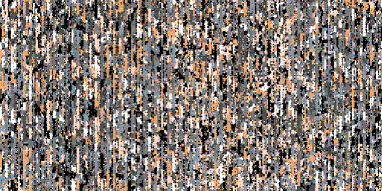
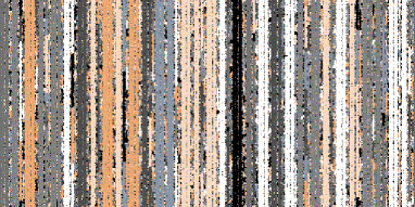
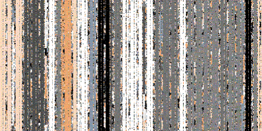
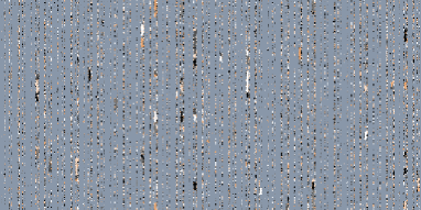
Figure 1: Typical Monte Carlo configurations (system of size $256\times 512$) in the high-temperature phase ($K_{0}=0.3$), in the neighbourhood of the critical point ($K_{0}=0.5$ and $K_{0}=0.6$), and in the low-temperature phase ($K_{0}=0.7$). The layered structure of the system is clearly visible.

Particular choices of coupling distribution make it possible to determine exactly the critical point by duality arguments BercheChatelainBerche98 . Consider a system of $N$ layers with a distribution $\{f_{k}\}$, made from a succession of vertical-horizontal (V-H) bonds when read from left to right (Fig. 2), and let us write its singular free energy density $f_{s}(K_{0},K_{1};\{f_{k}\})$. Under a duality transformation, the strong and weak couplings $K_{i}$ are, respectively, replaced by weak and strong dual couplings $\tilde{K}_{i}$, where ${\rm e}^{\tilde{K}_{i}}-1=q/({\rm e}^{K_{i}}-1)$. Since a vertical bond on the original lattice becomes horizontal on the dual system, the same V-H bond configuration is recovered for the transformed system when the distribution is read from right to left, and one gets the same type of system, but a reverse distribution $\{f_{L+1-k}\}$. The free energies of the two systems are equal: $f_{s}(K_{0},K_{1};\{f_{k}\})=f_{s}(\tilde{K}_{0},\tilde{K}_{1};\{f_{L+1-k}\})$. The sequences considered here have the property that the reverse distribution corresponds to the original one after exchange of perturbed and unperturbed couplings $K_{1}\leftrightarrow K_{0}$:

$$f_{s}(\tilde{K}_{0},\tilde{K}_{1};\{f_{L+1-k}\})=f_{s}(\tilde{K}_{1},\tilde{K}_{0};\{f_{k}\}).$$ (5)

The system being thus self-dual, the critical point, if unique, is exactly given by the critical line $(K_{0})_{c}=(\tilde{K}_{1})_{c}$ of the usual anisotropic model Fisch78 ; KinzelDomany81 :

$$({\rm e}^{K_{c}}-1)({\rm e}^{K_{c}r}-1)=q.$$ (6)

One should mention that the required symmetry property of the sequences possibly holds after omitting the last digit which simply introduces an irrelevant surface effect.

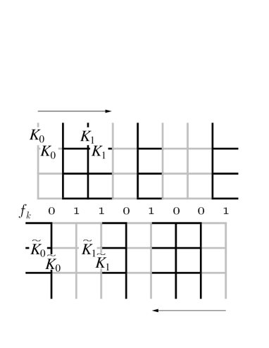
Figure 2: Layered structure of the system and its transformation under duality (above). The critical line in the coupling space is also shown (below).

The fluctuations of the coupling strengths per bond at the correlation length scale $\xi$ induce a thermal perturbation $\langle\delta t\rangle\sim t^{-\nu(\omega-1)}$, which has to be compared to the deviation from the critical point $t$. The resulting perturbation has a crossover exponent $\Phi=1+\nu(\omega-1)$ and is relevant when $\Phi>0$. This criterion, first obtained by Luck Luck93 , founds its justification at a critical point, i.e. when the correlation length of the pure system diverges as the transition point is approached. The question of its application at first-order phase transitions is not yet clear. The purpose of this paper is to report some results in this situation. The eight-state Potts model has the advantage of undergoing a strong first-order transition in the pure case, and has been already intensively studied by several techniques with random bonds ChenFerrenbergLandau95 ; CardyJacobsen97 ; ChatelainBerche98 .

In the following, we consider three different aperiodic sequences and a periodic system (PS) with the regular succession of couplings $K_{1}$, $K_{0}$, $K_{1}$, $K_{0},\dots$, in which the transition is surely first-order. This system constitutes a reference for the first-order type behaviour and presents the advantage of having the same value for the critical coupling (at fixed $r$) than the aperiodic sequences considered. The substitution rules for the aperiodic sequences studied in the paper are given in Table 1.

Table 1: Substitution rules for the aperiodic sequences considered in the text.

Sequence		substitutions	wandering
			exponent
Thue-Morse	(TM):	$0\to 01,$	$\omega_{\rm TM}=-\infty$
		$1\to 10.$
Paper-Folding	(PF):	$00\to 1000,$	$\omega_{\rm PF}=0$
		$01\to 1001,$
		$10\to 1100,$
		$11\to 1101.$
Three-Folding	(TF):	$0\to 010,$	$\omega_{\rm TF}=0$
		$1\to 011.$

Details on their properties can be found in ref. TurbanIgloiBerche94 ; BercheBercheTurban96 . We first performed preliminary runs (to be presented in the next section) for different values of the temperature, and then intensive Monte Carlo simulations at criticality on two-dimensional square lattices of sizes $L\times 4L$ (PF, TM, PS) or $L\times 3L$ (TF), using the Swendsen-Wang cluster algorithm SwendsenWang87 . This technique is known to be very efficient to study second-order phase transitions, since it is less affected by the critical slowing down than conventional Metropolis algorithm. At first-order phase transition points, other methods can be used to improve the effectiveness, but we favoured the use of the same algorithm to study the different regimes, increasing the number of Monte Carlo iterations when necessary in order to obtain reliable results. The multi-spin coding technique has also been used to speed up the simulations CreutzJacobsRebbi81 . The geometry $L\times pL$ allows a sufficiently large number of rows in order to explore the aperiodic structure at long enough length scales and the value of $p$ has been chosen with respect to the symmetries of the sequences. The boundary conditions are periodic in the short direction ($L$) and free or fixed in the long direction ($pL$).

Table 2: Details of the typical parameters used in the Finite-Size Scaling Monte Carlo simulations^a and energy auto-correlation time in the case $r=5$. Sizes $L=2^{n}$ or $3^{n}$ between the limits indicated in the table have been used.

Sequence	size(b)	$\#$ MCS/spin(c)	$\tau_{E}$
			min.	max.
PS	8 to 256	$2.10^{5}$ to $3.10^{6}$	7.3	651.1
TM	8 to 2048	$1.10^{5}$ to $4.10^{6}$	6.7	141.4
PF	8 to 2048	$3.10^{5}$ to $4.10^{5}$	6.7	8.8
TF	3 to 2187	$2.10^{5}$ to $2.5\ 10^{5}$	4.5	18.2

^a5000 iterations (in MCS/spin) have been discarded. ^bThe values indicated correspond to the largest size $pL$ (horizontal direction) with $p=4$ (PS, TM, PF) and $p=3$ (TF). ^cThe same numbers of MC iterations have been used for the two types of boundary conditions (free and fixed in the horizontal direction).

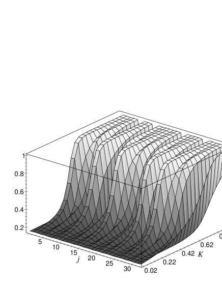
Figure 3: Temperature dependence of the order parameter profile in the case of the Thue-Morse sequence.

With these boundary conditions, translational invariance holds in the vertical direction, and a local order parameter is defined by the majority orientation of the spins at column $j$ ChallaLandauBinder86 :

$$m(j)=\frac{q\rho_{\rm max}(j)-1}{q-1},\quad M_{j}\equiv\langle m(j)\rangle.$$ (7)

Here, $\rho_{\rm max}(j)={\rm max}_{\sigma}[\rho_{\sigma}(j)]$, where $\rho_{\sigma}(j)$ is the density of spins in the state $\sigma$ at column $j$ and $\langle\dots\rangle$ denotes the thermal average over the Monte Carlo iterations. The systems under consideration are highly inhomogeneous, as it can be seen in Fig. 3, so, in order to reduce fluctuations, we studied average quantities, e.g.

$$m=\frac{q\rho_{\rm max}-1}{q-1},\quad M\equiv\langle m\rangle,$$ (8)

where $\rho_{\rm max}$ has the same meaning as above, over the whole system and is not restricted to a given row. The susceptibility is obtained as usually via the fluctuations of magnetization $\chi=KpL^{2}(\langle m^{2}\rangle-\langle m\rangle^{2})$, and we also computed the energy density

$$E=\frac{1}{2KpL^{2}}\left\langle\sum_{(i,j)}K_{ij}\delta_{\sigma_{i},\sigma_{j}}\right\rangle,$$ (9)

where the prefactor ensures a normalization to 1. Local properties at the surface have also been calculated, e.g. $M_{1}=\langle m(1)\rangle$.

3 Off-critical point behaviour

In this section, we give a qualitative description of the order of the phase transition. For this purpose, we performed preliminary MC simulations over a range of values of $K$ for a system of size $L\times 2L$ ($L$ from 8 to 256, TM and PF sequences), and determined the temperature dependence of the physical quantities. The behaviour of the average magnetization, susceptibility, and Binder cumulant of the magnetization for the TM and PF sequences at $r=5$ are shown in Fig. 4 and Fig. 5, respectively.

Figure 4: Temperature dependence of the average magnetization, susceptibility, and magnetization cumulant for the TM sequence ($r=5$). The different symbols correspond to simulations of systems of sizes $8\times 16$ ($\circ$) to $256\times 512$ ($\times$).

Figure 5: Temperature dependence of the average magnetization, susceptibility, and magnetization cumulant for the PF sequence ($r=5$). The different symbols correspond to simulations of systems of sizes $8\times 16$ ($\circ$) to $256\times 512$ ($\times$).

Figure 6: Rescaled susceptibility with respect to the size-dependent critical coupling $K_{c}(L)$ for TM and PF sequences at $r=5$. Three sizes ($64\times 128$, $128\times 256$ and $256\times 512$) have been used. In the case of TM, one observes a behaviour which approaches a $\delta$-function, while a power-law is obtained for PF.

As well known in Monte Carlo simulations, it is difficult to observe, in the numerical data, a jump of the order parameter at the transition point of a first-order phase transition, and similarly the $\delta$-like behaviour of the susceptibility cannot easily be distinguished from a pure power-law, so we report here also the results for the magnetization cumulant Vollmayretal93 . As a consequence of the highly inhomogeneous systems under consideration, these cumulants exhibit a quite complicated structure, but their behaviour already gives an idea of the nature of the transition for the two sequences. One can indeed observe in Fig. 4 (TM) that a narrow well appears in the vicinity of the transition point and becomes deeper as the system size increases. This should be the signature of a first-order phase transition, while in Fig. 5 (PF) there is no analogous significant trend. The direct comparison between the two sequences also shows that the variation of the magnetization and of the susceptibility close to the critical coupling is sharper for TM than PF.

A criterion to analyse the order of phase transitions, from the observation of the way the non-analytic behaviour develops as the critical point is approached, has recently been proposed Meyer-OrtmannsReisz98 . Singular quantities, like the susceptibility, are response functions with diverging non-analytic behaviour in the thermodynamic limit. In the scaling region, there exists a certain interval where such functions are decreasing at first-order transitions, leading to crossings of the rescaled curves which evolve towards a $\delta$-like behaviour, while they increase with the size of the system in the neighbourhood of $K_{c}$ at second-order transitions (power-law behaviour). This is illustrated in Fig. 6 where the case of Thue-Morse sequence belongs to the first situation, while Paper-Folding corresponds to the second one. For this latter perturbation, typical Monte Carlo simulations are shown in Fig. 1. In the disordered phase, the layered structure of the correlated clusters becomes appearent as the system approaches the transition point, where these clusters begin to grow in the perpendicular direction, leading to a second order critical point in the thermodynamic limit.

Similar qualitative observations were reported in Ref. BercheChatelainBerche98 , where temperature-dependent effective exponents, for average magnetization and susceptibility, were computed by comparing the data at two different sizes $L$ and $L^{\prime}=L/2$: In the case of the magnetization for example, assuming a scaling form $M_{L}(t)=L^{-\beta/\nu}{\cal M}(Lt^{\nu})$, where $t=\mid\!K-K_{c}\!\mid$ and ${\cal M}(x)$ is a scaling function, the quantity

$${X}_{L}(t)=\frac{\ln M_{L}/M_{L^{\prime}}}{\ln L/L^{\prime}}.$$ (10)

expanded in powers of $Lt^{\nu}$ close to $K_{c}$ leads to

$${X}_{L}(t)\simeq-\frac{\beta}{\nu}+\frac{Lt^{\nu}}{2\ln 2}\frac{{\cal M}^{\prime}(Lt^{\nu})}{{\cal M}(Lt^{\nu})}+O(L^{2}t^{2\nu}),$$ (11)

which defines an effective exponent which evolves towards $-\frac{\beta}{\nu}$ as the critical point is approached and in the thermodynamic limit. In the case of the TM sequence, the successive estimates of $\frac{\beta}{\nu}=d-y_{h}$ and $\frac{\gamma}{\nu}=2y_{h}-d$ evolve towards the values 0 and 2. This is characteristic of a first-order phase transition, since the scaling dimensions associated to the temperature and magnetic field, $y_{t}$ and $y_{h}$, respectively, take a special value equal to the dimension $d$ of the system FisherBerker82 . In the case of the PF sequence, the behaviour is drastically different, and these effective exponents evolve towards non trivial values around 0.5 and 1.

4 Finite-Size Scaling

4.1 Dynamical exponent

The conjectures of the previous section have to be confirmed by a FSS analysis. As well known in Monte Carlo simulations, the energy auto-correlation time $\tau_{E}$ is a good test to know about the order of the transition. In Table 2, we have given the characteristic values of $\tau_{E}$ for different sequences and sizes at the critical point. The number of MC iterations is always of order $10^{4}\tau_{E}$ to ensure reliable results. The autocorrelation time is shown in Fig. 7 in a semi-logarithmic scale.

Figure 7: Energy autocorrelation time $\tau$ at $K_{c}$ ($r=5$). For TM, the dashed line is a fit to an exponential behaviour, while it is a power-law fit for PF ($z\sim-0.04$) and TF ($z\sim 0.12$) sequences. The data corresponding to the periodic system have not been fitted.

The numerical data for PF and TF sequences can be fitted by a power-law $\tau_{E}\sim L^{z}$, with a very small dynamical exponent presumably linked to a logarithmic behaviour, while in the case of TM, $\tau_{E}$ is exponentially diverging $\tau_{E}\sim L^{d/2}{\rm e}^{2\sigma L^{d-1}}$ where $\sigma$ is an order-disorder interface tension. These results support strong evidences that in the case of Paper-Folding and Three-Folding sequences, the fluctuations are strong enough to soften the transition to a second-order regime. In the case of Thue-Morse, even if the autocorrelation time, compared to the periodic case, is lowered by the fluctuations, the transition remains first-order. We note that the data corresponding to the PS were not fitted since one has to go to strongly first order transitions ($q=15$) to observe the predicted exponential behaviour in the pure system Gupta .

4.2 Bulk properties

We can now enter upon a more refined characterization of the phase transition in the two regimes. Since the critical point is exactly known, FSS techniques are well indicated to get accurate results. We made different series of simulations with free-free ($f|f$), fixed-fixed ($F|F$), and mixed ($f|F$) or ($F|f$) boundary conditions (BC) in the horizontal direction. From all simulations we can extract the singular behaviour of the magnetization and of the susceptibility, since there is no regular contribution and, at the critical point we can write

$$M(K_{c},L)={\cal A}_{M}L^{-\beta/\nu},$$ (12)

$$\chi(K_{c},L)={\cal A}_{\chi}L^{\gamma/\nu},$$ (13)

where ${\cal A}_{X}$ are non-universal critical amplitudes. On the other hand, the four series of simulations are necessary in order to extract the singularity associated to the energy density which contains a regular part including both a bulk $E^{(0)}$ and a surface $E^{(-1)}\times L^{-1}$ contribution BercheBercheTurban96 ; KarevskiLajkoTurban97 . This latter part must be split in two terms, since the two surfaces are different. We thus have 

$$E_{(l|r)}(K_{c},L) = E^{(0)}(K_{c},L)$$ (14)

$$+ (E^{(-1)}_{l}(K_{c},L)+E^{(-1)}_{r}(K_{c},L))\times L^{-1}$$

$$+ {\cal A}_{(l|r)}L^{(\alpha-1)/\nu}+\dots$$

where $(l|r)$ specifies the BC’s (free or Fixed) for the left and right surfaces. We note that our simulations being performed in a cylinder geometry, the Euler number vanishes, and thus there is no $\ln L$ term in the free energy CardyPeschel88 ; Cardy88 . The asymptotic values of the bulk energy density with different BC’s are the same in the thermodynamic limit, but the amplitudes of the finite-size corrections being different, the regular contributions cancel in the combination:

$$\Delta E(K_{c},L) = E_{(F|F)}+E_{(f|f)}-E_{(f|F)}-E_{(F|f)}$$

$$= [{\cal A}_{(F|F)}+{\cal A}_{(f|f)}-{\cal A}_{(f|F)}-{\cal A}_{(F|f)}]L^{(\alpha-1)/\nu}$$

leaving a pure power-law.

The scaling dimensions can be deduced from log-log plots of the different quantities vs. the system size. In the case of the Thue-Morse sequence, a crossover appears, as the size increases, towards a behaviour which resembles the periodic one, characterized by a vanishing exponent for the magnetization. This effect is visible in Fig. 8 where the evolution of size-dependent effective exponents is shown. Similarly, after the crossover regime, the susceptibility is described by an exponent $\gamma/\nu$ close to the value $d=2$. The behaviour of the energy density difference exhibits log-periodic oscillations, characteristic of systems with discrete scale invariance. It makes more difficult a quantitative analysis, but a tendency to a decreasing slope for the largest size is nevertheless observed.

Certainly, a careful analysis is needed to avoid the crossover effects from small sizes to the true fixed point behaviour in the infinite lattice size limit, so we define the following procedure: From the log-log curves between $pL_{\rm min}$ and $pL_{\rm max}$, one determines an effective exponent $x(L_{\rm min})$ for each quantity; then the smaller size is canceled from the data and the whole procedure is repeated until only the three or four largest sizes remain. The effective exponent is then plotted against $L_{\rm min}^{-1}$. This prescription makes appearent the crossover effects and enables us to identify unambiguously the asymptotic regime. Different values of the aperiodic perturbation ($r=0.2$, 5, and 10) are shown in Fig. 8 in the case of TM sequence. At small sizes, the system is still strongly under the influence of the fluctuations induced by the aperiodic distribution of couplings, while as the size increases, the effective exponents converge towards trivial values which are characteristic of a first-order regime. The ratio $\beta/\nu=0$ is indeed characteristic of a discontinuity of the order parameter, while $\gamma/\nu=2$ is consistent with this discontinuity and with the scaling law $2\beta/\nu+\gamma/\nu=d$. This behaviour of effective exponents is the signature that the aperiodic fluctuations are eventually irrelevant. This is corroborated by the fact that the crossover takes place at larger sizes when the perturbation amplitude becomes stronger ($r=10$).

Figure 8: Effective size-dependent exponents associated to the susceptibility and magnetization in the case of TM sequence for different values $r=K_{1}/K_{0}=0.2$, 5, and 10, of the coupling ratio (Note that $r=0.2$ corresponds to a perturbation of the same strength than $r=5$). The error bars correspond to the standard deviations of the corresponding power-law fits.

On the contrary, the two other aperiodic sequences exhibit power-law behaviours with non-trivial exponents. Since a second-order phase transition occurs for these sequences, the question of the stability of the new fixed point has to be considered. A numerical study at different ratios of interactions $r=0.2$, 2, 3, 5, and 10 shows that the corresponding exponents remain stable for strong enough perturbations ($r$ not too close to the pure system value 1).

The numerical results of power-law fits in the linear part of log-log plots are given in Table 3 for PS, TM, PF and TF sequences.

Table 3: Bulk critical exponents obtained by the slope of finite-size scaling results for the fours sequences. The numbers in parentheses give the estimated uncertainty in the last digit.

	PS		TM
	$\beta/\nu$	$\gamma/\nu$	$\beta/\nu$	$\gamma/\nu$
$r=0.2$	0.046(6)	2.01(1)	0.10(3)	1.81(7)
$r=5.$	0.072(4)	1.97(1)	0.08(2)	1.90(5)
$r=10.$	0.045(2)	2.02(1)	cross.a	cross.
	PF		TF
	$\beta/\nu$	$\gamma/\nu$	$\beta/\nu$	$\gamma/\nu$
$r=2.$	0.464(7)	1.13(2)	–b	–
$r=3.$	0.475(8)	1.07(2)	–	–
$r=5.$	0.480(3)	1.017(9)	0.43(2)	1.15(2)
$r=10.$	0.49(1)	1.01(1)	0.44(2)	1.09(3)
$r=0.2$	0.46(1)	1.04(2)	0.43(1)	1.15(2)
	$(1-\alpha)/\nu$
	PS	TM	PF	TF
$r=5.$	0.05(4)	osc.c	1.015(4)	osc.

^a “cross.” means that the crossover is still too strong to allow any linear regime in the log-log plots. ^b The symbol – means that the corresponding runs have not been performed. ^c “osc.” means that the log-periodic oscillating behaviour does not allow any precise estimation of the exponent.

Since the values deduced from these power-law fits seem to remain stable with respect to the perturbation amplitude, we can use the effective exponents (Fig. 9) to determine a more accurate value of the critical exponents deduced from the extrapolation at infinite size. The results are given in Table 4 for all sequences at $r=5$, for which value we have the more exhaustive numerical results. Log-periodic oscillations again appear in the behaviour of the energy density combination in the TF sequence, but the tendency is coherent with the behaviour of PF sequence.

Figure 9: Effective size-dependent exponents associated to the susceptibility, magnetization, and energy density difference (dotted line: PS, dot-dashed line: TM, long-dashed line: TF, and solid line: PF) for $r=5$. Arrows on the right of the figure demarcate the curves corresponding to $\gamma/\nu$ and $-\beta/\nu$.

Table 4: Bulk critical exponents obtained by extrapolation at infinite size of finite-size scaling results for the sequences PS, TM, PF and TF with a ratio $r=5$.

	PS	TM	PF	TF
$\beta/\nu$	$0.012$	$0.020$	$0.499$	$0.508$
$\gamma/\nu$	$1.986$	$1.993$	$0.995$	$1.009$
$(1-\alpha)/\nu$	$0.05$	osc.a	$1.001$	osc.

^a “osc.” means that the log-periodic oscillating behaviour does not allow any precise estimation of the exponent.

From these values of the critical exponents, we can deduce the scaling dimensions associated to the temperature and the magnetic field, $y_{t}=d-\frac{1-\alpha}{\nu}\approx 1.00$ and $y_{h}=d-\frac{\beta}{\nu}=\frac{d+\gamma/\nu}{2}\approx 1.50$ at the new fixed point for PF and TF. It could be surprising to obtain, within the precision of our results, the same fixed point for these aperiodic perturbations, but we can mention here that both of them have the same wandering exponent $\omega=0$.

4.3 Surface properties

The surface properties can also be investigated, and here we ask if the aperiodic perturbations are also liable to modify the surface critical behaviour. We determined numerically the value of the order parameter at both surfaces $j=1$ and $j=pL$ for the four sequences considered. It gives the corresponding exponents, called $\beta_{1}/\nu$ and $\beta_{pL}/\nu$, respectively. The log-log plots are shown in Fig. 10 and the exponents, deduced from the slopes of log-log plots in the linear regime, are given in Table 5.

Figure 10: Local surface magnetization at both ends of the system for the four sequences considered in the text. The curves have been shifted for clarity.

Table 5: Surface critical exponents^a obtained by the slope of finite-size scaling results for the four sequences.

	PS		TM
	$\beta_{1}/\nu$	$\beta_{4L}/\nu$	$\beta_{1}/\nu$	$\beta_{4L}/\nu$
$r=5.$	0.60(1)	0.59(1)	0.55(2)	osc.b
$r=10.$	0.60(1)	0.60(1)	cross.c	cross.
$r=0.2$	0.56(1)	0.61(1)	0.60(2)	osc.
	PF		TF
	$\beta_{1}/\nu$	$\beta_{4L}/\nu$	$\beta_{1}/\nu$	$\beta_{3L}/\nu$
$r=2.$	0.013(3)	0.58(1)	–d	–
$r=3.$	0.0023(6)	0.58(1)	–	–
$r=5.$	0.0000(0)	0.58(1)	0.530(4)	0.17(1)
$r=10.$	0.0000(0)	0.58(1)	0.532(2)	0.095(3)
$r=0.2$	0.54(1)	0.000(0)	0.19(1)	0.61(2)

^aThe numbers in parentheses give the estimated uncertainty in the last digit. ^b “osc.” means that the log-periodic oscillating behaviour does not allow any precise estimation of the exponent. ^c “cross.” means that the crossover is still too strong to allow any linear regime in the log-log plots. ^d The symbol – means that the corresponding runs have not been performed.

We can observe that the PS and TM systems exhibit analogous singularities at the surfaces. It is known in the pure case that, even with a first-order phase transition in the bulk of the system, a second-order phase transition is obtained at the surface. The critical exponents keep constant values around 0.6 independently of the interaction ratio $r$. In the case of PF and TF sequences, a second-order regime which depends on the coupling ratio is obtained. The transition is strenghtened when the coupling are sufficiently enhanced, and one can even observe a first-order transition (in the case of PF) at the surface. This result can be understood by the behaviour of the average coupling at a length scale $n$ in the vicinity of the left surface for example, $\bar{K}_{n}$, compared to the asymptotic average coupling $\bar{K}_{\infty}$:

$$R_{n}=\frac{\bar{K}_{n}}{\bar{K}_{\infty}}=\frac{\rho_{n}(r-1)+1}{\rho_{\infty}(r-1)+1},\quad\rho_{n}=\frac{1}{n}\sum_{k=1}^{n}f_{k}.$$ (16)

This ratio is always greater than 1 when $r>1$ for PF and produces a significative enhancement of the interactions close to the boundary, leading to a decrease of the exponent of the surface magnetization. The contrary happens with TF as shown in Fig. 11. We have also checked that these exponents are characteristic not only of the local boundary behaviour, but also of an average surface property, since the average of the order parameter over a few rows (from 2 to 10) in the vicinity of the surface reproduces the same exponents.

Figure 11: Average coupling at a length scale $n$ from the left surface for the sequences PF, TM and TF ($r=2$). The interactions are enhanced, on average, close to the surface for PF, while they are reduced for TF, and remain constant in the case of TM.

4.4 Crossover effect or marginal variation of the exponents for PF and TF sequences?

The question one poses in this section is whether the small observed variations of the critical exponents in the second-order phase transition regime results from a crossover effect or from a marginal behaviour. It is interesting here to make a comparison with what occurs in the Ising model case $q=2$. For this model, the PF and TF sequences are known to lead to a marginal behaviour with continuoulsy varying critical exponents. The surface properties of this system have been intensively investigated BercheBercheTurban96 ; IgloiTurbanKarevskiSzalma97 , but the coupling distribution used here being different from the one used in previous works, we cannot directly compare the values of the exponents. We performed a few simulations for $q=2$, and the results are given in Table 6. It appears clearly that the values of the different critical exponents exhibit, as expected, a continuous variation with the amplitude of the interactions. The aim of these supplementary simulations is to show unambiguously that a marginal variation of the exponents is strong enough to be distinguished numerically from the crossover effect at small perturbations. Our results suggest that the small variation observed in the Potts model case is probably due to this latter situation.

Table 6: Bulk and surface critical exponents^a obtained by the slope of finite-size scaling results for PF sequences in the case of the Ising model $q=2$.

$r$	$\beta/\nu$	$\gamma/\nu$	$\beta_{1}/\nu$	$\beta_{4L}/\nu$
0.2	0.337(2)	1.37(1)	0.497(1)	0.0203(4)
5	0.360(2)	1.351(9)	0.0176(7)	0.517(3)
10	0.407(1)	1.233(6)	0.0044(2)	0.525(4)

^aThe numbers in parentheses give the estimated uncertainty in the last digit.

5 Conclusion

In this paper, we have shown that the deterministic fluctuations generated by an aperiodic modulation of nearest-neighbour couplings in the eight-state Potts model produce a softening of the transition, and are even liable to induce a second-order phase transition. It happens when the fluctuations around the average coupling are strong enough, and it is the case for the Paper-Folding and Three-Folding sequences, although they are characterized by a vanishing wandering exponent. In the case of the Thue-Morse sequence, the wandering exponent being $-\infty$, the transition remains of first-order, and the scaling dimensions keep their pure values. These results are consistent with Luck’s criterion Luck93 , provided that we replace the correlation-length exponent $\nu$ by its trivial value $1/y_{t}=1/d$ at the first-order fixed point. The crossover exponent associated to the aperiodic distribution $\Phi=1+(\omega-1)/d$ is then positive (relevant perturbation) for PF and TF sequences while it is negative (irrelevant) in the case of TM sequence.

The analysis of the bulk properties shows that the new fixed point exponents (PF and TF) are stable, i.e. do not depend, up to small crossover effects, on the value of the perturbation amplitude. This is clearly different from the marginal behaviour encountered for similar sequences in the Ising model case. We can furthermore notice that the new universality class seems to be robust, i.e. the same for both sequences, a result which is not a priori obvious. One can nevertheless mention that our results are coherent with the stability of the new fixed point, which requires a non-positive value for the crossover exponent $\Phi^{\prime}$ in the second-order regime. With $\omega=0$, $\Phi^{\prime}$ takes the value $\Phi^{\prime}=1-\nu$ at the new fixed point. Using hyperscaling relation $\alpha=2-d\nu$ (which should hold, unless anisotropic behaviour is found), the value $\alpha\simeq 0$, obtained numerically for PF, leads to $\nu\simeq 1$ and thus $\Phi^{\prime}\simeq 0$. It seems reasonable to propose a renormalization group sketch, illustrated by the evolution of the effective exponents, where the two possible sets of exponents should correspond to two different fixed points, the stability of which depend on the strength of fluctuations (i.e. the value of the wandering exponent). The two types of situations are shown in Fig 12. The periodic system, as it can be seen in Fig 9, is not influenced by the existence of the second fixed point.

Figure 12: Evolution of the size-dependent effecive exponents for the two types of aperiodic sequences.

The surface magnetization has also been analyzed and analogous conclusions can be given. It is interesting to notice that a first-order surface transition (with a second-order regime in the bulk) can be induced in the case of PF, i.e. the exact contrary of the pure model behaviour.

There are still some open questions concerning aperiodic perturbations in these systems. A possible anisotropic scaling behaviour could be obtained in the second-order induced regime, since it occurs in the Ising model already. One should also investigate aperiodic sequences with diverging fluctuations characterized by a positive wandering exponent, like Rudin-Shapiro for example. A second-order transition should also be obtained, but its universality class could be different.

- (1)
- (2) A. Aharony, J. Magn. Magn. Mater. 7, 198 (1978).
- (3) T. C. Lubensky, in Ill-condensed matter, Ecole d’été de Physique Théorique, Les Houches 31e session, R. Balian, R. Maynard and G. Toulouse eds. (North Holland Publishing Company, Amsterdam, 1978), p. 405
- (4) C. Itzykson and J.M. Drouffe, Théorie Statistique des Champs, vol. 2, (InterEditions ; Editions du CNRS, Paris 1989), chap. 10.
- (5) J. L. Cardy, Scaling and Renormalization in Statistical Physics (Cambridge University Press, Cambridge, 1996), chap. 8.
- (6) R. Brout, Phys. Rev. 115, 824 (1959).
- (7) S.-K. Ma, Modern Theory of Critical Phenomena (Benjamin, Reading, 1976), chap. 10.
- (8) A. B. Harris, J. Phys. C 7, 1671 (1974).
- (9) Y. Imry and M. Wortis, Phys. Rev. B 19, 3580 (1979).
- (10) Y. Imry and S.-K. Ma, Phys. Rev. Lett. 35, 1399 (1975).
- (11) A. N. Berker, Phys. Rev. B 29, 5293 (1984).
- (12) M. Aizenman and J. Wehr, Phys. Rev. Lett. 62, 2503 (1989).
- (13) K. Hui and A. N. Berker, Phys. Rev. Lett. 62, 2507 (1989).
- (14) A. N. Berker, J. Appl. Phys. 70, 5941 (1991).
- (15) A. N. Berker, Physica A 194, 72 (1993).
- (16) S. Chen, A. M. Ferrenberg, and D. P. Landau, Phys. Rev. Lett. 69, 1213 (1992).
- (17) F.Y. Wu, Rev. Mod. Phys. 54, 235 (1982).
- (18) S. Chen, A. M. Ferrenberg, and D. P. Landau, Phys. Rev. E 52, 1377 (1995).
- (19) J. L. Cardy and J. L. Jacobsen, Phys. Rev. Lett. 79, 4063 (1997).
- (20) C. Chatelain and B. Berche, Phys. Rev. Lett. 80, 1670 (1998).
- (21) M. Picco, cond-mat/9802092 Preprint
- (22) D. Shechtman, I. Blech, D. Gratias, and J. W. Cahn, Phys. Rev. Lett. 53, 1951 (1984).
- (23) U. Grimm and M. Baake, The Mathematics of Long-Range Aperiodic Order, R. V. Moody ed. (Kluwer, Dordrecht, 1996), p. 199.
- (24) J. M. Luck, Europhys. Lett. 24, 359 (1993).
- (25) F. Iglói, J. Phys. A 21, L911 (1988).
- (26) M. M. Doria and I. I. Satija, Phys. Rev. Lett. 60, 444 (1988).
- (27) C. A. Tracy, J. Phys. A 21, L603 (1988).
- (28) V. G. Benza, Europhys. Lett. 8, 321 (1989).
- (29) M. M. Doria, F. Nori, and I. I. Satija, Phys. Rev. B 39, 6802 (1989).
- (30) L. Turban, F. Iglói, and B. Berche, Phys. Rev. B 49, 12 695 (1994).
- (31) F. Iglói and L. Turban, Europhys. Lett. 27, 91 (1994).
- (32) D. Karevski, G. Palágyi, and L. Turban, J. Phys. A 28, 45 (1995).
- (33) P. E. Berche and B. Berche, Phys. Rev. B 56, 5276 (1997).
- (34) P. E. Berche, B. Berche, and L. Turban, J. Phys. (France) I 6, 621 (1996).
- (35) F. Iglói and P. Lajkó, J. Phys. A 29, 4803 (1996).
- (36) F. Iglói, L. Turban, D. Karevski, and F. Szalma, Phys. Rev. B 56, 11 037 (1997).
- (37) D. Ledue, D. P. Landau, and J. Teillet, in Computer Simulation Studies in Condensed-Matter Physics, Vol. X, D. P. Landau, K. K. Mon, and H. B. Schüttler eds. (Springer, Berlin, 1997).
- (38) P. E. Berche, C. Chatelain, and B. Berche, Phys. Rev. Lett. 80, 297 (1998).
- (39) M. Queffélec, in Substitution Dynamical Systems, Lecture Notes in Mathematics Vol. 1294, A. Dold and B. Eckmann eds. (Springer, Berlin, 1987), p. 97.
- (40) R. Fisch, J. Stat. Phys. 18, 111 (1978).
- (41) W. Kinzel and E. Domany, Phys. Rev. B 23, 3421 (1981).
- (42) R. H. Swendsen and J. S. Wang, Phys. Rev. Lett. 58, 86 (1987).
- (43) M. Creutz, L. Jacobs, and C. Rebbi, Comput. Phys. Commun. 23, 337 (1981).
- (44) A. M. Ferrenberg and R. H. Swendsen, Phys. Rev. Lett. 61, 2635 (1988).
- (45) A. M. Ferrenberg and R. H. Swendsen, Phys. Rev. Lett. 63, 1195 (1989).
- (46) M. S. S. Challa, D. P. Landau, and K. Binder, Phys. Rev. B 34, 1841 (1986).
- (47) K. Vollmayr, J. D. Reger, M. Scheucher, and K. Binder, Z. Phys. B 91, 113 (1993).
- (48) H. Meyer-Ortmanns and T. Reisz, hep-lat/9802020 Preprint
- (49) M. E. Fisher and A. N. Berker, Phys. Rev. B 26, 2507 (1982).
- (50) S. Gupta, Phys. Lett. B325, 418 (1994).
- (51) D. Karevski, P. Lajkó, and L. Turban, J. Stat. Phys. 86, 1153 (1997).
- (52) J. L. Cardy and I. Peschel, Nucl. Phys. B 300[FS22], 377 (1988).
- (53) J. L. Cardy, in fields, strings and critical phenomena, Les Houches 1988, E. Brézin and J. Zinn-Justin eds. (North-Holland, Amsterdam 1990), p. 169.
- (54) E. Buffenoir and S. Wallon, J. Phys. A 26, 3045 (1993).