Spectral function and quasiparticle weight in the generalized $t-J$ model

Abstract

We extend to the spectral function an approach which allowed us to calculate the quasiparticle weight for destruction of a real electron $Z_{c\sigma}({\bf k)}$ (in contrast to that of creation of a spinless holon $Z_{h}({\bf k)}$) in a generalized $t-J$ model, using the self-consistent Born approximation (SCBA). We compare our results with those obtained using the alternative approach of Sushkov et al., which also uses the SCBA. The results for $Z_{c\sigma}({\bf k)}$ are also compared with results obtained using the string picture and with exact diagonalizations of a 32-site square cluster. While on a qualitative level, all results look similar, our SCBA approach seems to compare better with the ED one. The effect of hopping beyond nearest neighbors, and that of the three-site term are discussed.

]

I Introduction

The momentum distribution function of holes in a quantum antiferromagnetic background has been a subject of considerable interest since the discovery of high-$T_{c}$ systems. Reliable information on these quantities was obtained from the exact diagonalization of the $t-J$ model in small clusters [1, 2, 3, 4, 5]. An analytical approximation which brings considerable insight into the underlying physics is based on the string picture [6]. Within the string picture, for realistic $t>J$, the movement of the hole can be separated into a fast motion around a fixed position $j$ on the lattice (to which the hole is attracted by a string potential caused by the distortion of the Neel background), and a slow motion of $j$ due essentially to spin fluctuations which restore the Neel background as $j$ is displaced. The resulting quasiparticle weight as a function of wave vector $Z_{c\sigma}({\bf k)}$ for one hole, agrees very well with exact diagonalizations (ED) of a $4\times 4$ cluster [6]. However, this cluster is still too small and finite-size effects are important [4, 5].

Another successful analytical approach is the self-consistent Born approximation (SCBA) [7, 8, 9, 10, 11]. The resulting dispersion of one hole in the $t-J$ model is in very good agreement with exact diagonalizations of small clusters [5, 9, 10], including a square cluster of 32 sites, which contains the most important symmetry points and smaller finite-size effects in comparison with previous calculations [5]. The SCBA has also been used to calculate the doping dependence of the superconducting critical temperature $T_{c}$ in qualitative agreement with experiment [12]. However, due to the particular representation used (see Eq. (4) below), the Green function which results from the SCBA is that of a spinless holon $G_{h}$, while the real particle becomes related with a composite operator $c_{k\sigma}$ (composed of a holon and a spin deviation). The holon quasiparticle weights $Z_{h}({\bf k)}$ differ from $Z_{c\sigma}({\bf k)}$ which are the physical quantities calculated by ED and accessible to experiment. Only recently, motivated by photoemission experiments in insulating Sr₂CuO₂Cl₂ [13], two approaches appeared which relate $Z_{c\sigma}$ [14] and the Green function of the physical hole $G_{c\sigma}$ [15] with $G_{h}$ within the framework of the SCBA. In addition, to fit accurately the experimentally observed dispersion, it is necessary to include second- $(t_{2})$ and third-nearest-neighbor hopping $(t_{3})$ to the $t-J$ model [16, 17], and to explain qualitatively the observed intensities, it is necessary to consider the strong-coupling limit of a Hubbard model [14, 18]. This implies that a three-site term $t^{\prime\prime}=-J/4$ should be included in the model, and the one-particle operators should be transformed. While a generalized Hubbard model is able to provide a consistent picture of the observed charge and and spin excitations in Sr₂CuO₂Cl₂ [19], we must warn that the effective strong-coupling low-energy effective model derived from a realistic multiband model [20, 21, 22, 23], although also includes $t_{2}$ and $t_{3}$, can have a different $t^{\prime\prime}$, even of opposite sign, favoring instead of suppressing of $d$-wave superconductivity and a resonance-valence-bond ground state [24, 25, 26, 27].

For future theoretical studies, as well as to compare with photoemission [13, 28, 29], or other experiments (like electron-energy-loss spectroscopy [30, 31]) it is important to compare the four above mentioned approaches to calculate the quasiparticle dispersion and intensities, trying to establish their relative accuracy or convenience. This is the main purpose of this work.

In Section 2 we derive an expression for the spectral density of the physical hole $\rho_{c\sigma}=-$Im$G_{c\sigma}/\pi$ in terms of the Green function of the spinless hole $G_{h}$ within the SCBA, and briefly describe the alternative expression derived by Sushkov et al. [15] for $G_{c\sigma}$. Section 3 contains a comparison of both resulting $\rho_{c\sigma}({\bf k,}\omega)$ after solving the SCBA equations. In Section 4, we compare the results for $Z_{c\sigma}({\bf k)}$ obtained using both SCBA approaches with ED results for the $t-J$ model [5], and those derived from a string picture [6]. In Section 5 we include $t_{2}$, $t_{3}$ and $t^{\prime\prime}$ and compare recent ED results for the 32-site cluster [32] with the SCBA ones. Section 6 contains the conclusions.

II Green function of a physical hole within the SCBA

We consider the dynamics of one hole in a square lattice described by a generalized $t-J$ model:

$$H = -\sum_{i\delta\sigma}t_{\delta}c_{i+\delta\sigma}^{{\dagger}}c_{i\sigma}+{\frac{J}{2}}\sum_{i\eta}({\bf S}_{i}\cdot{\bf S}_{i+\eta}-{\frac{1}{4}}n_{i}n_{i+\eta})$$ (2)

$$+t^{\prime\prime}\sum_{i\eta\neq\eta^{\prime}\sigma}c_{i+\eta^{\prime}\sigma}^{{\dagger}}c_{i+\eta\sigma}({\frac{1}{2}}-2{\bf S}_{i}\cdot{\bf S}_{i+\eta}).$$

The first term contains hopping to first, second and third nearest neighbors with parameters $t_{1},~{}t_{2},~{}t_{3}$ respectively. The nearest neighbors of site $i$ are labeled as $i+\eta$. In the SCBA, long-range antiferromagnetic order is assumed, and a spinless fermion $h_{i}$ at each site is introduced [7, 8, 9, 10, 11]. Calling A (B) the sublattice of positive (negative) spin projections in the Neel state, one can use the following representation:

$$c_{i\uparrow} = h_{i}^{\dagger},\,\,\,\,\,\,\,\,\,c_{i\downarrow}=h_{i}^{\dagger}a_{i}\,,\,\,\,\,\,\text{if }\,\,i\in\,\text{A}$$ (3)

$$c_{i\uparrow} = h_{i}^{\dagger}a_{i},\,\,\,c_{i\downarrow}=h_{i}^{\dagger}\,\,,\,\,\,\,\,\,\,\,\,\,\text{if}\,\,\,\,i\in\,\text{B,}$$ (4)

where $a_{i}^{\dagger}$ creates a spin deviation at site $i$ in the Neel state, and there is a constraint that at the same site there cannot be both, a hole and a spin deviation. This constraint is neglected [9]. The exchange part of Eq. (1) is diagonalized by a standard canonical transformation, and retaining only linear terms in the spin deviations for the other terms, the Hamiltonian takes the form:

$$H = \sum_{q}\omega_{q}\alpha_{q}^{\dagger}\alpha_{q}+\sum_{k}\epsilon_{k}h_{k}^{\dagger}h_{k}$$ (6)

$$+\frac{4t_{1}}{\sqrt{N}}\sum_{kq}M({\bf k,q})(h_{k}^{\dagger}h_{k-q}\alpha_{q}+\text{H.c.}),$$

where $\alpha_{q}=u_{q}a_{q}-v_{q}a_{q}^{\dagger}$, $\omega_{q}=2J\,\nu_{q},$ $\epsilon_{k}=(t_{2}+2(1-x)t^{\prime\prime})\epsilon_{2}(k)+(t_{3}+(1-x)t^{\prime\prime})\epsilon_{1}(2k)$ $x=1/N$ is the doping, $\epsilon_{1}(k)=4\gamma_{k}$, $\epsilon_{2}(k)=4$ cos $k_{x}$ cos $k_{y}$,

$$v_{q}^{2} = u_{q}^{2}-1=\frac{1}{2\nu_{q}}-\frac{1}{2},\ \nu_{q}=(1-\gamma_{q}^{2})^{1/2},$$ (7)

$$\gamma_{q} = (\cos q_{x}+\cos q_{y})/2,\ \text{sgn}(v_{q})=\text{sgn}(\gamma_{q}),$$ (8)

$$M({\bf k,q}) = u_{q}\gamma_{k-q}+v_{q}\gamma_{k},$$ (9)

and $u_{q}>0$.

From the Hamiltonian Eq.(6), the SCBA allows to calculate the holon Green function $G_{h}$ accurately through the self-consistent solution of the following two equations:

$$\Sigma({\bf k},\omega) = \frac{z^{2}t_{1}^{2}}{N}\sum_{q}M^{2}({\bf k,q})G_{h}({\bf k-q},\omega-\omega_{q})$$ (10)

$$\,\,\,\,\,\,\,\,\,\,\,\,\,\,\,\,\,\,\,\,G_{h}^{-1}({\bf k},\omega) = \omega-\epsilon_{k}-\Sigma({\bf k},\omega)+i\epsilon.$$ (11)

$z=4$ is the coordination number.

However, the physical operator is the Fourier transform of $c_{i\sigma}$ and since it is a composite operator in the representation Eq.(4), it is not trivial to find its Green function $G_{c\sigma}$. Recently, two different approaches to calculate the quasiparticle weight $Z_{c\sigma}({\bf k)}$ [14] and the whole Green function $G_{c\sigma}({\bf k},\omega)$ [15] using the SCBA have been proposed. Here we extend to the spectral density $\rho_{c\sigma}({\bf k,}\omega)=-$Im$G_{c\sigma}({\bf k,}\omega)/\pi$ our previous derivation [14]. We assume for the moment that the system is finite and its eigenvalues are discrete. The idea is to relate $G_{c\sigma}$ and $G_{h}$, using the equation of motion [33] to find the wave function for each eigenvector. If $|\psi_{k}^{n}\rangle$ is an eigenstate of Eq. (6) with total wave vector k and other quantum numbers labeled by $n$, it can be expanded as:

$$|\psi_{k}^{n}\rangle = A_{0}^{n}({\bf k})h_{k}^{\dagger}|0\rangle+\frac{1}{\sqrt{N}}\sum_{q}A_{1}^{n}({\bf k,q})h_{k-q}^{\dagger}\alpha_{q}^{\dagger}|0\rangle$$ (13)

$$+\frac{1}{N}\sum_{q_{1},q_{2}}A_{2}^{n}({\bf k,q}_{1},{\bf q}_{2})h_{k-q_{1}-q_{2}}^{\dagger}\alpha_{q_{2}}^{\dagger}\alpha_{q_{1}}^{\dagger}|0\rangle+...,$$

and the Schrödinger equation $(\lambda_{k}^{n}-H)|\psi_{k}^{n}\rangle=0$, leads to an infinite set of equations for the $A_{i}^{n}$. Neglecting some terms not described by the SCBA [33], the first two of these equations are:

$$A_{0}^{n}({\bf k})(\lambda_{k}^{n}-\epsilon_{k})=\frac{1}{N}\sum_{q}A_{1}^{n}({\bf k,q})M({\bf k,q})$$ (14)

$$A_{1}^{n}({\bf k,q})(\lambda_{k}^{n}-\epsilon_{k-q}-\omega_{q})\simeq zt_{1}[A_{0}^{n}({\bf k})M({\bf k,q})$$ (15)

$$+\frac{1}{N}\sum_{q_{2}}A_{2}^{n}({\bf k,q},{\bf q}_{2})M({\bf k-q,q}_{2})].$$ (16)

A solution of the set of approximate equations can be solved relating $A_{i}^{n}$ with $A_{i-1}^{n}$ [33]. In particular, if

$$A_{2}^{n}({\bf k,q},{\bf q}_{2}) = zt_{1}A_{1}^{n}({\bf k,q})M({\bf k-q,q}_{2})$$ (18)

$$\times G_{h}({\bf k-q-q}_{2},\lambda_{k}^{n}-\omega_{q}-\omega_{q_{2}}),$$

with $G_{h}({\bf k},\omega)$ and $\Sigma({\bf k},\omega)$ satisfying Eqs. (11), from Eqs. (16) it follows that:

$$A_{1}^{n}({\bf k,q})=zt_{1}A_{0}^{n}({\bf k})M({\bf k,q})G_{h}({\bf k-q},\lambda_{k}^{n}-\omega_{q}),$$ (19)

and the eigenvalue equation:

$$A_{0}^{n}({\bf k})[\lambda_{k}^{n}-\epsilon_{k}-\Sigma({\bf k},\lambda_{k}^{n})]=0\text{.}$$ (20)

Since we are considering the case of only one hole at zero temperature (otherwise Eqs. (11) have to be generalized [34, 35]), the relevant Fock space is composed by $|0\rangle$ (the ground state of the Heisenberg antiferromagnet), and the eigenstates with one added hole $|\psi_{k}^{n}\rangle$. In this restricted Hilbert space, the Lehmann representations [34, 35] of the relevant Green functions read:

$$G_{c\sigma}({\bf k},\omega) = \sum_{n}\frac{|\langle\psi_{k}^{n}|c_{k\sigma}|0\rangle|^{2}+|\langle\psi_{k+(\pi,\pi)}^{n}|c_{k\sigma}|0\rangle|^{2}}{\omega-\lambda_{k}^{n}+i\epsilon},$$ (21)

$$G_{h}({\bf k},\omega) = \sum_{n}\frac{|\langle\psi_{k}^{n}|h_{k}^{\dagger}|0\rangle|^{2}}{\omega-\lambda_{k}^{n}+i\epsilon}.$$ (22)

Using Eqs. (4) and the expression of the $a_{i}$ in terms of the magnon operators $\alpha_{q}$ to Fourier transform $c_{i\sigma}$ [14], Eqs.(13), (19), (22), and some algebra, we find for the ratio of spectral functions:

$$\frac{\rho_{c\sigma}({\bf k,}\omega)}{\rho_{h}({\bf k,}\omega)}=\frac{1}{2}|1+\frac{2zt_{1}}{N}\sum_{q}^{\prime}v_{q}M({\bf k,q})G_{h}({\bf k-q},\omega-\omega_{q})|^{2},$$ (23)

where the sum runs over all wave vectors of the antiferromagnetic Brillouin zone, excluding ${\bf q=0}$, and $v_{q}$ and $M({\bf k,q})$ are given by Eq. (9).

Although Eq. (23) has been derived assuming that the eigenvalues are discrete, we expect it to be also valid for a continuum distribution of energy levels (the incoherent background of the spectrum), or in other words, when the small imaginary part $i\epsilon$ in Eqs. (11) and (23) is larger than the average spacing between the levels. This seems to be confirmed by the results shown in the next section. A similar method of using the Schrödinger equation assuming discrete eigenvalues was used to obtain the non-interacting Green function of the Anderson model [36].

Sushkov et al. [15] used a different method to relate $G_{c\sigma}({\bf k},\omega)$ with $G_{h}({\bf k},\omega)$. They treat the operators $c_{k\sigma}$ as originated by an external perturbation to the Hamiltonian Eq. (6). This perturbation is characterized by two vertices in which the physical hole is transformed into a spinless hole $h_{k}^{\dagger}$, with or without exchange of a magnon. The physical Green function $G_{c\sigma}({\bf k},\omega)$ is obtained from a Dyson equation. Another difference with our approach lies in the different normalization of the operators $h_{k}^{\dagger}$, which is equivalent to another way of treating the constraint that there cannot be a hole and a spin deviation at the same site. We have neglected it since it has been shown that it does not affect the results for a quantum antiferromagnet (the situation is different if the spins are described by an Ising model) [9]. Sushkov et al. also have a factor $\sqrt{2}$ in their normalization of the $c_{k\sigma}$, which introduces a factor 2 in $G_{c\sigma}$. Dropping this factor to compare with other results, their final expression for the physical Green function reads:

$$G_{c\sigma}({\bf k},\omega)=0.4G_{h}({\bf k},\omega)+\frac{1}{N}\sum_{q}^{\prime}v_{q}^{2}G_{h}({\bf k-q},\omega-\omega_{q})$$ (24)

$$+4\sqrt{0.8}t_{1}G_{h}({\bf k},\omega)\frac{1}{N}\sum_{q}^{\prime}v_{q}M({\bf k,q})G_{h}({\bf k-q},\omega-\omega_{q})$$ (25)

$$+32t_{1}^{2}G_{h}({\bf k},\omega)[\frac{1}{N}\sum_{q}^{\prime}v_{q}M({\bf k,q})G_{h}({\bf k-q},\omega-\omega_{q})]^{2},$$ (26)

where $v_{q}$ and $M({\bf k,q})$ are given by Eq. (9).

III Comparison of spectral densities within SCBA.

The expression of the spectral density of the physical hole $\rho_{c\sigma}({\bf k,}\omega)$ derived from Eq. (26) is quite different from Eq. (23). Nevertheless, in both cases it is necessary first to solve numerically the SCBA Eqs. (11) to obtain the Green function of the spinless hole $G_{h}({\bf k},\omega)$. To perform this task with high accuracy, we have discretized the frequencies in intervals of $\Delta\omega=10^{-4}t_{1}$ and have taken the small imaginary part as $\epsilon=5\Delta\omega$. We have chosen a cluster of $16\times 16$ sites.

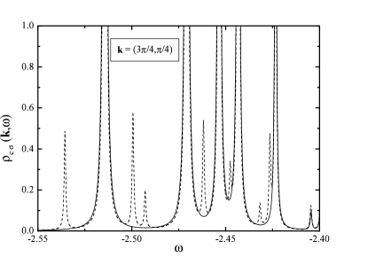
FIG. 1.: Spectral function of the physical hole obtained from the SCBA for wave vector k$=(3\pi/4,\pi/4)$. Full line: result of Eq.(12). Dashed line: result derived from the Dyson Eq. (13) [13]. Parameters are $t_{1}=1,~{}J=0.3,~{}t_{2}=-0.3,$ $t_{3}=0.2,$ $t^{\prime\prime}=0$.

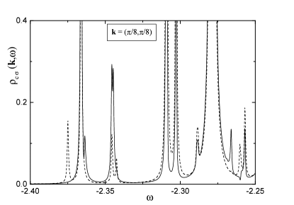
FIG. 2.: Same as Fig. 1 for k$=(\pi/8,\pi/8)$.

In Figs. 1 and 2, we represent the resulting spectral densities for a wave vector k at the boundary of the antiferromagnetic Brillouin zone, and another one near the zone center respectively. Except for wave vectors near $(\pi,\pi)$ at frequencies near the quasiparticle pole, the contribution of the term in $t_{1}$ in Eq. (23) is small compared to 1, and as a rough first approximation Eq. (23) gives $\rho_{c\sigma}({\bf k,}\omega)\simeq\rho_{h}({\bf k,}\omega)/2$. Thus, the result of our Eq. (23) looks qualitatively similar to the known results for $\rho_{h}$ within the SCBA [9, 10]. There are several peaks which can be qualitatively understood within the string picture as originated by different bound states of the string potential, which acquire dispersion as the center of the string potential is displaced by spin fluctuations or terms of sixth order in $t_{1}$ [6, 9]. The lowest peak corresponds to the coherent quasiparticle state. Note that the structure in the incoherent background displaying several different peaks cannot be resolved if the imaginary part in Eqs. (11) is as large as that used by Sushkov et al. ($\epsilon=0.1t_{1}$ [15]). The same happens for certain wave vectors and parameters with the quasiparticle peaks, when the quasiparticle energy $\lambda_{k}$ lies too near the incoherent background.

The result for $\rho_{c\sigma}({\bf k,}\omega)$ obtained using the Dyson Eq. (26) derived by Sushkov et al. [15] looks in general, and for any reasonable parameters of the generalized $t-J$ model, similar to ours, except for two differences: i) the intensity is a little bit smaller for the peaks already present in the spinless holon result $\rho_{h}({\bf k,}\omega)$ (see Fif. 1), ii) new peaks appear, which apparently do not have a physical meaning and seem to be an artifact of the approximations involved in the Dyson equation. In particular, except for high symmetry points of the Brillouin zone (like $(0,0)$, $(0,\pi)$ or $(\pi,\pi)$), for wave vectors k such that the quasiparticle energy $\lambda_{k}$ is near $\lambda_{(0,0)}$ (the bottom of the electron band), a new quasiparticle peak appears. Comparison with the position and intensity of the quasiparticle peak at k $=(3\pi/4,\pi/4)$ obtained from exact diagonalization of a square 32-site cluster [5, 32], described in the following two sections, confirm that this peak is spurious and is disregarded in the following.

IV Quasiparticle weights in the $t-J$ model

To obtain the quasiparticle intensity for each wave vector of the physical hole $Z_{c\sigma}({\bf k})$ within the SCBA, we have fitted the part of the spectral density (described by Eq. (23) or Eq. (26) and Eq. (9)) in the neighborhood of the quasiparticle peak by a sum of several Lorentzian functions. Since the imaginary part $\epsilon=5\times 10^{-4}t_{1}$ we have taken in the numerical solution of the SCBA Eqs. (11) is very small, we can isolate the quasiparticle peak (its width is practically identical to $2\epsilon$), even in some cases where the distance of this peak to the incoherent background is smaller than $\epsilon$. Integrating the corresponding Lorentzian we obtain $Z_{c\sigma}({\bf k})$. We have verified that using this method, finite-size effects are practically absent in our $16\times 16$ cluster. The peaks introduced by Eq. (26) which are absent in the spinless hole spectral density $\rho_{h}({\bf k,}\omega)$ were neglected.

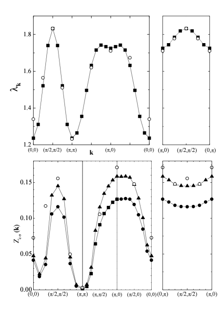
FIG. 3.: Top: quasiparticle energies obtained with the SCBA (solid squares). Bottom: corresponding quasiparticle weights obtained using Eq.(12) [12] (solid triangles) and from Dyson Eq. (13) [13] (solid circles). Open circles denote the corresponding results of an exact diagonalization (ED) of a square cluster of 32 sites [3]. Parameters are $t_{1}=1,~{}J=0.3,~{}t_{2}=t_{3}=t^{\prime\prime}=0$.

In Fig. 3 we compare quasiparticle energies $\lambda_{k}$ and weights $Z_{c\sigma}({\bf k})$ with those obtained from an exact diagonalization (ED) of a square cluster of 32 sites [5]. The SCBA results for $\lambda_{k}$ were already published [10]. We inverted the sign of $\lambda_{k}$ (the electron instead of the hole representation is used) in the following, in order to facilitate comparison with previous calculations and experiment. We also shifted the $\lambda_{k}$ in order that they coincide for the ground-state wave vector ${\bf k}=(\pi/2,\pi/2)$, as in Ref. [5]. The agreement between ED and SCBA results for $\lambda_{k}$ is excellent along the boundary of the antiferromagnetic Brillouin zone. However, there are some discrepancies near the zone center, particularly for ${\bf k}=(0,0)$ and ${\bf k}=(\pi/4,\pi/4)$. We ascribe this to finite-size effects, since in the thermodynamic limit $\lambda_{k}=\lambda_{k+(\pi,\pi)}$, due to the folding of the Brillouin zone caused by the antiferromagnetic symmetry breaking. Except for the above mentioned two wave vectors, the disagreement between the results for $Z_{c\sigma}({\bf k})$ of the ED and our SCBA approach [14] (Eq. (23)) is less than 7%. Using instead the SCBA expression (26) of Sushkov et al. [15], we obtain a quasiparticle weight which is $\sim 20\%$ below our results. Previous comparison of ED results for $Z_{c\sigma}({\bf k})$ on a square cluster of 20 sites [4] and SCBA results on a $20\times 20$ cluster using Eq. (23), also agreed very well except at ${\bf k}=(0,0)$.

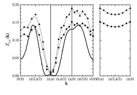
FIG. 4.: Quasiparticle weights obtained with the SCBA using Eq.(12) [12] (solid triangles) and Eq. (13) [13] (solid circles). The full thick line corresponds to results of the string picture scanned from Ref. 4. Parameters are $t_{1}=1,~{}J=0.4,~{}t_{2}=t_{3}=t^{\prime\prime}=0$.

Comparison between results of ED for clusters between 16 and 32 sites [4, 5], suggest that finite-size effects are very important for the $4\times 4$ cluster. In Fig. 4 we compare the results for $Z_{c\sigma}({\bf k})$ obtained using the string picture, scanned from Ref. [6] with both SCBA approaches. ED results on large enough clusters are not available for these parameters. While the three curves look qualitatively similar, it seems that the string picture results underestimate $Z_{c\sigma}({\bf k})$, particularly at ${\bf k}=(0,0)$ and near ${\bf k}=(\pi,\pi)$.

V Quasiparticle energies and weights in the generalized $t-J$ model

In this Section, we compare results for $\lambda_{k}$ and $Z_{c\sigma}({\bf k})$ which we obtained using the SCBA, with corresponding recent ED results, in which hoppings beyond nearest neighbors $t_{2},$ $t_{3}$ and the three-site term $t^{\prime\prime}$ were included [32]. A motivation to include these terms is that the inclusion of $t_{2}$ and $t_{3}$ is necessary [16, 17] to explain the experimentally observed dispersion in insulating Sr₂CuO₂Cl₂ [13]. However, to explain qualitatively the observed quasiparticle intensities, it is necessary to include at least Hubbard corrections to the relevant operators [14, 15, 18]. Their effect can be included in any theoretical approach and its main effect is to increase the intensities near the Brillouin zone center [14, 15, 18].

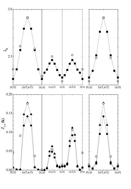
FIG. 5.: Same as Fig. 3 for the parameters of Fig. 1. The ED results were taken from Ref. 25.

Fig. 5 contains the results for $t^{\prime\prime}=0$. Comparing with Fig. 3 one can see that the effect of $t_{2}$ and $t_{3}$ is mainly to shift $\lambda_{(\pi,0)}$ towards the incoherent background, and as a consequence, the weight $Z_{c\sigma}(\pi,0)$ is strongly reduced. The same happens for neighboring k. Also, the agreement between ED and SCBA results for $\lambda_{k}$ near ${\bf k}=(\pi,0)$ is not so good as for $t_{2}=t_{3}=0$. In spite of this, the agreement between ED and SCBA results for $Z_{c\sigma}({\bf k})$ is still very good except at the points ${\bf k}=(0,0)$, ${\bf k}=(\pi/4,\pi/4)$ and ${\bf k}=(3\pi/4,3\pi/4)$, for which finite-size effects are present in the ED calculations as evidenced by the fact that $\lambda_{k}\neq\lambda_{k+(\pi,\pi)}$. In Fig. 6, we include the three-site term $t^{\prime\prime}=-J/4$, with magnitude corresponding to the strong-coupling limit of the Hubbard model. Its effect is to lower the quasiparticle energies $\lambda_{k}$ near the wave vectors $(0,0)$ and $(\pi,0)$, increasing the total dispersion. While the comparison between SCBA and ED results for $\lambda_{k}$ is not affected appreciably by $t^{\prime\prime}$, the corresponding weights $Z_{c\sigma}({\bf k})$ clearly disagree for wave vectors $(\pi/2,0)$ and ($\pi,\pi/2)$. However, the agreement between weights on the boundaries of the antiferromagnetic Brillouin zone continues to be satisfactory.

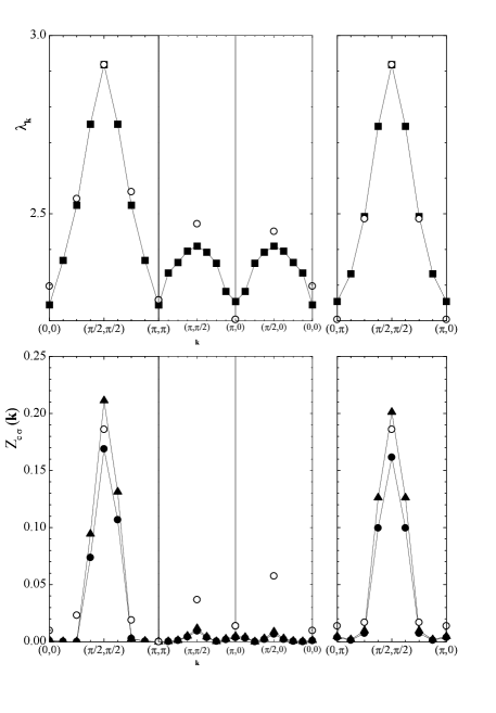
FIG. 6.: Same as Fig. 5 for $t^{\prime\prime}=-J/4$.

VI Summary and discussion

We have derived an expression which relates the spectral density of a physical hole with spin $\rho_{c\sigma}({\bf k,}\omega)$, with that of a spinless hole $\rho_{h}({\bf k,}\omega)$, and calculated it within the self-consistent Born approximation (SCBA). Another approach for the Green function of the physical hole, proposed by Sushkov et al. [15], introduces additional structure and spurious quasiparticle peaks in $\rho_{c\sigma}({\bf k,}\omega)$ for some wave vectors k. However, they can be identified and eliminated by comparison with the results obtained for $\rho_{h}$ within the SCBA.

We have also compared the SCBA quasiparticle energies $\lambda_{k}$ and weights $Z_{c\sigma}({\bf k})$ with available exact-diagonalization (ED) results on a square cluster of 32 sites for different parameters [5, 32], and with calculations using the string picture [6]. On a qualitative level, both SCBA approaches [14, 15], the string picture, and the ED results are similar. Quantitatively, although the string picture is very useful to give insight into the underlying physics, it seems that it underestimates the weights. The SCBA approach of Sushkov et al. [15] looks more accurate, but for all parameters and wave vectors studied here, the resulting $Z_{c\sigma}({\bf k})$ is smaller than the corresponding ED result and our SCBA one [14].

The agreement between $Z_{c\sigma}({\bf k})$ obtained from ED and our SCBA approach is very good, particularly for the $t-J$ model except at two k points where finite-size effects are evident in the ED results, and on the boundary of the antiferromagnetic Brillouin zone. In general, the $Z_{c\sigma}({\bf k})$ are larger if the corresponding $\lambda_{k}$ are near $\lambda_{(\pi/2,\pi/2)}$ (which correspond to the ground state for all parameters studied here). Inclusion of other hopping terms shifts $\lambda_{k}$, particularly for ${\bf k}\sim(\pi,0)$ away from $\lambda_{(\pi/2,\pi/2)}$, the corresponding weights $Z_{c\sigma}({\bf k})$ decrease, and the agreement between SCBA and ED results becomes poor for some of these wave vectors. This disagreement might be due to the fact that a nearest-neighbor hopping of the chosen sign weakens the antiferromagnetic long-range order [22, 23, 37, 38, 39]. While the existence of this order is an essential assumption of the SCBA, and is true for one hole in an infinite system, it is destroyed for a small finite concentration of holes $\sim 0.015$ in cuprates [40]. This concentration is smaller than the corresponding one (1/32) in the ED studies. Another possibility for the discrepancies is that vertex corrections which seem to not affect essentially the spinless hole Green function $G_{h}$ [11], become important for $Z_{c\sigma}({\bf k})$, particularly when the three-site term $t^{\prime\prime}$ is present.

For a quantitative comparison with photoemission experiments, it is necessary to transform the relevant operators of the appropriate multiband model, involving oxygen and copper orbitals, into those of the effective generalized $t-J$ model. This task might be performed generalizing previous related studies [41, 20, 21, 43].

REFERENCES

- [1] K. v. Szcepanski, P. Horsch, W. Stephan, and M. Ziegler, Phys. Rev. B 41 (1990) 2017.
- [2] V. Elser, D.A. Huse, B.I. Shraiman, and E.D. Siggia, Phys. Rev. B 41 (1990) 6715.
- [3] E. Dagotto, R. Joynt, A. Moreo, S. Bacci, and E. Gagliano, Phys. Rev. B 41 (1990) 9049.
- [4] D. Poilblanc, T. Ziman, H.J. Schulz, and E. Dagotto, Phys. Rev. B 47 (1993) 14267.
- [5] P.W. Leung and R.J. Gooding, Phys. Rev. B 52 (1995) R15711; 42 (1995) 711 (E).
- [6] R. Eder and K.W. Becker, Phys. Rev. B 44 (1991) 6982.
- [7] S. Schmitt-Rink, C.M. Varma, and A.E. Ruckenstein, Phys. Rev. Lett. 60 (1988) 2793.
- [8] C.L. Kane, P.A. Lee, and N. Read, Phys. Rev. B 39 (1988) 6880.
- [9] G. Martínez and P. Horsch, Phys. Rev. B 44 (1991) 317.
- [10] Z. Liu and E. Manousakis, Phys. Rev. B 45 (1992) 2425.
- [11] J. Bala, A.M. Oleś, and J. Zaanen, Phys. Rev. B 52 (1995) 4597.
- [12] N.M. Plakida, V.S. Oudovenko, P. Horsch, and A.I. Liechtenstein, Phys. Rev. B 55 (1997) R11997.
- [13] B.O. Wells, Z.-X. Shen, A. Matsuura, D.M. King, M.A. Kastner, M. Greven, and R.J. Birgeneau, Phys. Rev. Lett. 74 (1995) 964.
- [14] F. Lema and A.A. Aligia, Phys. Rev. B 55 (1997) 14092.
- [15] O.P. Sushkov, G.A. Sawatzky, R. Eder, and H. Eskes, Phys. Rev. B 56 (1997) 11769.
- [16] V.I. Belinicher, A.L. Chernyshev, and V.A. Shubin, Phys. Rev. B 54 (1996) 14914.
- [17] T. Xiang and J.M. Wheatley, Phys. Rev. B 54 (1996) R12653.
- [18] H. Eskes and R. Eder, Phys. Rev. B 54 (1996) 14226.
- [19] F. Lema, J. Eroles, C.D. Batista and E. Gagliano, Phys. Rev. B 55 (1997) 15289.
- [20] L.F. Feiner, J.H. Jefferson, and R. Raimondi, Phys. Rev. Lett. 76 (1996) 4939; references therein.
- [21] A.A. Aligia, F. Lema, M.E. Simon, and C.D. Batista, ibid 79 (1997) 3793; references therein.
- [22] A.A. Aligia, M.E. Simon, and C.D. Batista, Phys. Rev. B 49 (1994) 13061.
- [23] J. Eroles, C.D. Batista, and A.A. Aligia, Physica C 261 (1996) 237.
- [24] C.D. Batista and A.A. Aligia, Physica C 261 (1996) 237.
- [25] C.D. Batista, L.O. Manuel, H.A. Ceccatto, and A.A. Aligia, Europhys. Lett. 38 (1997) 147.
- [26] C.D. Batista and A.A. Aligia, J. Low Temp. Phys. 105 (1996) 591.
- [27] F. Lema, C.D. Batista and A.A. Aligia, Physica C 259 (1996) 287.
- [28] D.S. Marshall, D.S. Dessau, A.G. Loeser, C.H. Park, A.Y. Matsuura, J.N. Eckstein, I. Bozovik, P. Fournier, A. Kapitulnik, W.E. Spicer, and Z.X. Shen, Phys. Rev. Lett. 76 (1996) 4841.
- [29] J.M. Pothuizen, R. Eder, M. Matoba, G. Sawatzky, N.T. Hien, and A.A. Menovsky, Phys. Rev. Lett. 78 (1997) 717.
- [30] Y.Y. Wang, F.C. Zhang, V.P. Dravid, K.K. Ng, M.V. Klein, S.E. Schnatterly, and L.L. Miller, Phys. Rev. Lett. 77 (1996) 1809.
- [31] T. Böske, O. Knauff, R. Neudert, M. Knupfer, M.S. Golden, G. Krabbes, J. Fink, H. Eisaki, S. Uchida, K. Odaka, and A. Kotani, J. Low Temp. Phys. 105 (1996) 335.
- [32] P.W. Leung, B.O. Wells, and R.J. Gooding, Phys. Rev. B 56 (1997) 6320.
- [33] G.F. Reiter, Phys. Rev. B 49 (1994) 1536.
- [34] G.D. Mahan, Many Particle Physics (Plenum Press, New York, 1981).
- [35] F. Lema, Ph. D. thesis, Universidad Nacional de Cuyo, Argentina (1997).
- [36] D.R. Hamann, Phys. Rev. 2 (1970) 1373.
- [37] T. Tohyama and S. Maekawa, Phys. Rev. B 46 (1994) 3596.
- [38] R.J. Gooding, K.J.E. Vos, and P.W. Leung, Phys. Rev. B 49 (1994) 4119.
- [39] R.J. Gooding, K.J.E. Vos, and P.W. Leung, Phys. Rev. B 50 (1994) 12866.
- [40] R. Birgeneau, Am. J. Phys. 58 (1990) 28; B. Keimer, N. Belk, R.J. Birgeneau, A. Cassanho, C.Y. Chen, M. Greven, M.A. Kastner, A. Aharony, Y. Endoh, R.W. Erwin, and G. Shirane, Phys. Rev. B 46 (1992) 14034.
- [41] C.D. Batista and A.A. Aligia, Phys. Rev. B 47 (1993) 8929; 49 (1994) 16048.
- [42] L. Feiner, Phys. Rev. B 48 (1993) 16857.
- [43] M.E. Simon, A.A. Aligia and E.R. Gagliano, Phys. Rev. B 56 (1997) 5637.