Fundamental measure theory for mixtures of parallel hard cubes.
II. Phase behaviour of the one-component fluid and of the binary mixture

Abstract

A previously developed fundamental measure functional [J. Chem. Phys.107, 6379 (1997)] is used to study the phase behaviour of a system of parallel hard cubes. The single-component fluid exhibits a continuous transition to a solid with an anomalously large density of vacancies. The binary mixture has a demixing transition for edge-length ratios below 0.1. Freezing in this mixture reveals that at least the phase rich in large cubes always lies in the region where the uniform fluid is unstable, hence suggesting a fluid-solid phase separation. A method is developed to study very asymmetric binary mixtures by taking the limit of zero size ratio (scaling density and fugacity of the solvent as appropriate) in the semi-grand ensemble where the chemical potential of the solvent is fixed. With this procedure the mixture is exactly mapped onto a one-component fluid of parallel adhesive hard cubes. At any density and solvent fugacity the large cubes are shown to collapse into a close-packed solid. Nevertheless the phase diagram contains a large metastability region with fluid and solid phases. Upon introduction of a slight polydispersity in the large cubes the system shows the typical phase diagram of a fluid with an isostructural solid-solid transition (with the exception of a continuous freezing). Consequences about the phase behaviour of binary mixtures of hard core particles are then drawn.

I Introduction

This paper is the sequel of a previous one[3] (henceforth referred to as I) in which the so-called fundamental measure theory (FMT) was applied to build a density functional for the multicomponent system of parallel hard cubes (PHC). In I we explained all fundamentals of the theory and gave a full account of the technical details involved in the derivation of the functional. We also discussed the pros and cons of the theory, as compared with more standard density functional theories (DFTs), and suggested some possible extensions.

In this paper we apply the formalism developed in I to study the phase behaviour of the PHC fluid, with special emphasis in its relevance for the understanding of the phase behaviour of mixtures. The PHC fluid is a rather academic model and it possesses a bunch of ‘peculiarities’ which are rather odd for a fluid model, e.g. the uniform fluid is anisotropic at small scales (the cubes are kept parallel to each other), freezing occurs at very low packing fractions (around 0.3–0.4) and it is a continuous, instead of first order, transition (a consequence of the lack of isotropy of the fluid phase), and the depletion in the binary mixture is very strong compared to hard spheres (HS). But in spite of these peculiarities—which certainly make of this model a caricature of a fluid, the physics one can learn from its phase behaviour can be easily extended to more reasonable fluids, and it has the important added value of being a much simpler model to carry out analytical calculations (even more: FMT seems to be somehow optimal for this model [3, 4]).

There have been a few previous studies in the literature about the fluid of PHC [5, 6, 7, 8, 9, 10] scattered in the last forty years, but the relevance of this model has only recently become apparent when it has been proposed as a model of a fluid able to demix by a purely entropic mechanism. [11, 12]

Entropic demixing has been a long standing question which only recently begins to be understood. It is well known that different attractions between two types of particles in a fluid can produce segregation into two phases, each rich in one type of particles. [13] The question remains whether hard particles, for which only an entropic balance can drive a phase transition, ever demix and how. It is clear that nonadditive mixtures (mixtures in which particles of different type interact as if they had a larger volume) do demix, [14, 15, 16, 17] but they have the segregation mechanism introduced at the interaction potential. So the nontrivial question concerns additive hard-particle mixtures. The question is tricky because the simplest model of this type—HS—was solved in Percus-Yevick (PY) approximation [18] and shown never to demix. [19] It had to wait almost thirty years until the PY result was questioned. By solving numerically the Ornstein-Zernike equation with closure relations more accurate than the PY one a spinodal instability was shown to occur in a binary mixture of HS [20, 21, 22] for a diameter ratio below 0.1–0.25 (depending of the authors).

It was then believed that a sufficiently asymmetric HS binary mixture undergoes fluid-fluid demixing in a certain region of the phase diagram. But successive experiments performed in suspensions of polystyrene or silica spheres (which to a large accuracy can be considered HS) showed cumulative evidence that demixing is coupled to freezing, and so one of the phases shows up as a crystal—sometimes a glass—of large particles. [23, 24, 25, 26] Recent theoretical calculations confirm this scheme. [27, 28]

Direct computer simulations have run into troubles when dealing with this problem due to the extremely low probability of moving a larger particle in a sea of small ones without overlapping any of them. Simulations are still possible for not too dissimilar diameters, but they do not show demixing. [29, 30] With the help of specially designed cluster moves the first evidence of demixing has recently been found in simulations for diameter ratios smaller than 0.05. [31] Unfortunately these cluster moves do not help above the percolation threshold, and this sets a relatively low upper bound for the total packing fraction of the fluid. Besides, this method does not allow to identify the coexisting phases, so it does not distinguish fluid-fluid or fluid-solid demixing.

In order to elucidate the nature of demixing for very asymmetric mixtures the attention has shifted to understand the depletion interaction. An effective pair potential between the large spheres can be obtained by different procedures. [32, 33, 34, 35] Its shape reveals a very deep and narrow (one small-sphere diameter) well followed by a couple of small oscillations extending two or three small-sphere diameters. The depth and the amplitude of the oscillations depend on the small spheres packing fraction. In view of the phase behaviour of spheres with narrow and deep attractive potentials [36, 37] fluid-fluid demixing is ruled out for sufficient asymmetry, and instead fluid-solid demixing or even expanded-dense solid demixing (i.e. demixing once the large component has crystallised) should appear. Simulations of a system of HS supplemented by the depletion potential [33, 34, 35] confirm this conjecture if the diameter ratio is below 0.1. Expanded-dense solid demixing is indeed shown in some of this simulations for ratios 0.1 [34] or 0.05. [35] This phase behaviour has been recently corroborated by direct simulations of the binary mixture, [38] which have been shown to be possible in the relevant region of the phase diagram thanks to the small amount of small spheres present in those statepoints.

In the limit of zero size of the small spheres at constant packing fraction the depletion potential becomes Baxter’s adhesive potential. [39, 40] By applying a similar limit to the FMT functional of a binary mixture of PHC [3, 4] we have recently obtained a functional for parallel adhesive hard cubes (PAHC). [41] By avoiding the singularities of this potential (we will treat this point in detail later on) we show that the phase behaviour of this fluid is consistent with the above described picture for the mixture of HS, with the difference that expanded-dense solid demixing is the most common scenario because PAHC freezing occurs at rather low packing fractions.

II The one-component fluid

There are relatively few results in the literature concerning the fluid of PHC. As concerns the uniform fluid the virial coefficients, both in 2D and 3D, have been exactly obtained through diagrammatic expansions up to the seventh. [5, 6] They have also been obtained for different approximate integral equation theories. [7] The main consequence one draws from this information is that the virial expansion is very poorly convergent. For the 3D fluid, the seventh order virial expansion exhibits a maximum in the pressure at $\eta\approx 0.6$, and then goes down very quickly to reach negative values. [7] Its behaviour at moderate densities strongly deviates from that of a sixth order virial expansion—in contrast with what happens for HS. This is the fingerprint of a nearby divergence. In fact, the simulations of the fluid of PHC (3D) [8, 9] show a continuous freezing into a simple cubic lattice at [9] $\eta=0.48\pm 0.02$ (in contrast with the first order nature of the HS freezing). This result has been proven to be exact in infinite dimensions. [10] The reason for a continuous freezing is the lack of rotational symmetry of this system even in the disordered phase [10] (thus freezing does not brakes this symmetry). Allowing the cubes to rotate restores the first order nature of the freezing transition. [9]

FMT’s equation of state of the uniform PHC fluid is simply that of the scaled particle theory (SPT), i.e., from Eqs. (60) and (61) of I,

$$\beta P/\rho = \frac{1}{(1-\eta)^{2}}\,,\quad(D=2),$$ (1)

$$\beta P/\rho = \frac{1+\eta}{(1-\eta)^{3}}\,,\quad(D=3),$$ (2)

with $\beta$ the inverse absolute temperature in Boltzmann constant units, $P$ the pressure, $\rho$ the number density, and $\eta$ the packing fraction, $\eta=\rho\sigma^{D}$, $\sigma$ being the cube edge-length. In Fig. 1 the SPT equation of state (2) is compared with the simulation data.

On the other hand freezing can be studied as usual in DFT by parametrising the local density with a sum of gaussians centered at the lattice points. [42] Since the lattice is simple cubic, this can be easily achieved by setting

$$\rho({\bf r}) = \prod_{\nu=x,y,z}\sum_{n_{\nu}=-\infty}^{\infty}g(\nu-n_{\nu}d)\,,$$ (4)

$$g(u) \equiv \left(\frac{\alpha}{\pi}\right)^{1/2}e^{-\alpha u^{2}}\,,$$ (5)

with $d=\eta^{-1/3}\sigma$ the lattice spacing, and $\alpha$ a variational parameter determining the localisation of particles at the lattice sites.

In I we expressed the free-energy functional of a multicomponent system with density profiles $\rho_{i}({\bf r})$ ($i$ labeling the species) as

$$F[\{\rho_{i}({\bf r})\}] = F^{\rm id}[\{\rho_{i}({\bf r})\}]+F^{\rm ex}[\{\rho_{i}({\bf r})\}]\,,$$ (6)

$$\beta F^{\rm id}[\{\rho_{i}({\bf r})\}] = \sum_{i}\int d{\bf r}\,\rho_{i}({\bf r})\left[\ln{\cal V}_{i}\rho_{i}({\bf r})-1\right]\,,$$ (7)

$$\beta F^{\rm ex}[\{\rho_{i}({\bf r})\}] = \int d{\bf r}\,\Phi(\{n_{\alpha}({\bf r})\})\,,$$ (8)

with ${\cal V}_{i}$ the thermal volume of species $i$, and $n_{\alpha}=\sum_{i}\rho_{i}*\omega_{i}^{(\alpha)}$ a set of four weighted densities (stars denotes convolution) defined by the weights

$$\omega^{(0)}_{i} \equiv \delta_{i}^{x}\delta_{i}^{y}\delta_{i}^{z}\,,$$ (10)

$${\bf w}^{(1)}_{i} \equiv \bigl{(}\theta_{i}^{x}\delta_{i}^{y}\delta_{i}^{z},\delta_{i}^{x}\theta_{i}^{y}\delta_{i}^{z},\delta_{i}^{x}\delta_{i}^{y}\theta_{i}^{z}\bigr{)}\,,$$ (11)

$${\bf w}^{(2)}_{i} \equiv \bigl{(}\delta_{i}^{x}\theta_{i}^{y}\theta_{i}^{z},\theta_{i}^{x}\delta_{i}^{y}\theta_{i}^{z},\theta_{i}^{x}\theta_{i}^{y}\delta_{i}^{z}\bigr{)}\,,$$ (12)

$$\omega^{(3)}_{i} \equiv \theta_{i}^{x}\theta_{i}^{y}\theta_{i}^{z}\,,$$ (13)

with $\theta_{i}^{u}\equiv\Theta(\sigma_{i}/2-|u|)$, and $\delta_{i}^{u}\equiv(1/2)\delta(\sigma_{i}/2-|u|)$. As in I we will also need the two scalar densities $n_{i}=n_{i,x}+n_{i,y}+n_{i,z}$, $n_{i,\nu}$, $\nu=x,y,z$, being the vector components of ${\bf n}_{i}$, $i=1,2$. The function $\Phi({\bf r})$ is given in terms of the $n_{\alpha}$’s as (see I)

$$\Phi({\bf r})=-n_{0}\ln(1-n_{3})+\frac{{\bf n}_{1}\cdot{\bf n}_{2}}{1-n_{3}}+\frac{n_{2,x}n_{2,y}n_{2,z}}{(1-n_{3})^{2}}$$ (14)

with $n_{2,\nu}$, $\nu=x,y,z$, the components of ${\bf n}_{2}$.

For convenience let us introduce the functions

$$e(u) \equiv \frac{1}{2}\mbox{erf}\,\left(\sqrt{\alpha}u\right)\,,$$ (15)

$$p(u) \equiv \sum_{n=-\infty}^{\infty}[e(u-nd+\sigma/2)-e(u-nd-\sigma/2)]\,,$$ (16)

$$q(u) \equiv \sum_{n=-\infty}^{\infty}[g(u-nd+\sigma/2)+g(u-nd-\sigma/2)]$$ (17)

[notice that $g(u)=e^{\prime}(u)$]. The latter two are periodic with period $d$. In terms of these functions

$$n_{3} = p(x)p(y)p(z)\,,$$ (19)

$${\bf n}_{2} = \frac{1}{2}\bigl{(}q(x)p(y)p(z),p(x)q(y)p(z),p(x)p(y)q(z)\bigr{)}\,,$$ (20)

$${\bf n}_{1} = \frac{1}{4}\bigl{(}p(x)q(y)q(z),q(x)p(y)q(z),q(x)q(y)p(z)\bigr{)}\,,$$ (21)

$$n_{0} = \frac{1}{8}q(x)q(y)q(z)\,,$$ (22)

and accordingly $\Phi({\bf r})=n_{0}({\bf r})\psi({\bf r})$, where

$$\psi=-\ln(1-n_{3})+\frac{n_{3}}{1-n_{3}}+\frac{n_{3}^{2}}{(1-n_{3})^{2}}\,.$$ (23)

This simplification occurs because of the factorisation of the density (4)—and hence of (II).

The free energy per particle, $\Psi\equiv\beta F/N$, of the solid phase can be obtained as the integral over a unit cell of the lattice of the free energy density. Hence the ideal part turns out to be

$$\Psi^{\rm id} = \int_{-d/2}^{d/2}dx\int_{-d/2}^{d/2}dy\int_{-d/2}^{d/2}dz\,\rho({\bf r})[\ln{\cal V}\rho({\bf r})-1]$$ (24)

$$= \ln({\cal V}/\sigma^{3})-1$$ (26)

$$+3\int_{-\infty}^{\infty}dx\,g(x)\ln\left(\sum_{n=-\infty}^{\infty}\sigma g(x-nd)\right)\,.$$

The integrand is written in a suitable way to use Gauss-Hermite numerical quadratures. [43] As for the excess contribution, similar manipulations lead to

$$\Psi^{\rm ex} = \frac{1}{8}\int_{-d/2}^{d/2}dx\,q(x)\int_{-d/2}^{d/2}dy\,q(y)\int_{-d/2}^{d/2}dz\,q(z)\psi(x,y,z)$$ (27)

$$= \frac{1}{8}\int_{-\infty}^{\infty}dx\,g(x)\int_{-\infty}^{\infty}dy\,g(y)\int_{-\infty}^{\infty}dz\,g(z)$$ (29)

$$\times\sum_{\{\pm\}}\psi(x\pm\sigma/2,y\pm\sigma/2,z\pm\sigma/2)\,,$$

where the last summation runs over all combinations of signs. Again the latter expression is suitable for Gauss-Hermite integration, which is crucial this time because (29) involves a three-dimensional integration.

We can now minimise with respect to $\alpha$ to determine the equilibrium profile. This yields a continuous freezing at $\eta=0.348$. As the transition is continuous we can make a more accurate determination of the transition density via a standard bifurcation analysis. This is equivalent to finding the density at which the structure factor diverges for some wavevector ${\bf k}_{c}$. The structure factor is expressed in terms of the DCF as

$$S({\bf k})=\frac{1}{1-\rho\hat{c}({\bf k})}\,,$$ (30)

and the Fourier transform of the DCF, $\hat{c}({\bf k})$, is obtained through Eq. (56) of I for a one-component fluid. In order to simplify the final expression we exploit the symmetry of the crystal by choosing ${\bf k}_{c}=(k_{c},0,0)$ (the result would be the same if we chose $k_{c}$ along the Y or Z axes). Thus the condition to determine the critical point is

$$1 + 2\eta_{c}\frac{4-3\eta_{c}+\eta_{c}^{2}}{(1-\eta_{c})^{3}}j_{0}(k\sigma)$$ (31)

$$+ \eta_{c}^{2}\frac{9-4\eta_{c}+\eta_{c}^{2}}{(1-\eta_{c})^{4}}j_{0}(k\sigma/2)^{2}\geq 0\,,$$ (32)

the equality holding only for $k=k_{c}$; $j_{0}(x)\equiv\sin x/x$ is the zeroth order spherical Bessel function. The solution to this equation is $\eta_{c}=0.3143\dots$ and $k_{c}\sigma=4.8276\dots$.

It is noticeable the discrepancy between the value of $\eta_{c}$ obtained from the divergence of the structure factor and that obtained using the profile (II). The reason for this discrepancy can be inferred if we obtain from $k_{c}$ the lattice spacing, $d_{c}/\sigma=2\pi/k_{c}=1.3015\dots$; thus $\eta_{c}(d_{c}/\sigma)^{3}=0.6929\dots$, what means that the resulting crystal has a large fraction of vacancies (around 31% of the lattice sites!). This is a strong effect that can be accounted for by simply multiplying the r.h.s. of (4) by an average occupancy ratio $\vartheta$ and minimising with respect to this new variational parameter. In the calculation process this simply amounts to (i) add a term $\ln\vartheta$ to the ideal free energy (26), and (ii) replace $n_{3}$ by $\vartheta n_{3}$ in the definition of $\psi$ [Eq. (23)]. Notice that $d$ is now given by $d=\sigma(\vartheta/\eta)^{1/3}$. As a result we obtain the correct value of $\eta_{c}$ and an occupancy ratio of $\vartheta\approx 0.694$, consistent with the value obtained above. [44]

FIG. 1.: Equation of state of the PHC fluid. Solid lines correspond to the pressure of the stable phase (fluid or solid) at the given packing fraction, $\eta$. Dotted line is the unstable fluid branch beyond freezing. Dashed line is the solid branch computed without accounting for vacancies in the lattice (see text). Full circles are the simulations of Ref. [8] and empty circles those of Ref. [9] (actually we have averaged the two data sets reported for the largest system size).

The solid equation of state—with and without vacancies—is plotted in Fig. 1 and compared with the simulations. It is obtained as $\beta P\sigma^{3}=\eta^{2}\partial\Psi/\partial\eta$. We can see that the overall agreement is good, although the freezing point is shifted down with respect to the simulations because the SPT equation of state overestimates the pressure of the fluid phase.

III Stability of the binary fluid mixture

Two are the requirements for a fluid mixture to be stable: [45] (i) the positiveness of the specific heat at constant volume ($c_{V}$), and (ii) the positive definiteness of the matrix

$${\sf M}_{ij}\equiv\beta\frac{\partial^{2}f}{\partial\rho_{i}\partial\rho_{j}}\,,$$ (33)

where $f\equiv F/V$, $F$ being the Helmholtz free energy, and $\rho_{i}$ the number density of species $i$. Condition (i) is trivially fulfilled, because any hard core model is athermal, what means that the dependence of the free energy on temperature is that of an ideal gas; hence the positiveness of $c_{V}$. Condition (ii) is a consequence of the equilibrium state being a minimum of the free energy.

According to (8) the matrix M will be given by

$\displaystyle{\sf M}_{ij}=\beta\frac{\partial\mu_{j}}{\partial\rho_{i}}=\frac{1}{\rho_{i}}\delta_{ij}+\sum_{\alpha\gamma}\hat{\omega}^{(\gamma)}_{i}({\bf 0})\hat{\omega}^{(\alpha)}_{j}({\bf 0})\frac{\partial^{2}\Phi}{\partial n_{\gamma}\partial n_{\alpha}}\,,$

and relating the second term of the r.h.s. of this equation to the DCF of the fluid [Eq. (7) of I] it can simply be written as

$${\sf M}_{ij}=\frac{1}{\rho_{i}}\delta_{ij}-\hat{c}_{ij}({\bf 0})\,.$$ (34)

Now, for a binary mixture, M is a $2\times 2$ matrix with all its elements positive; thus the mixture will be stable provided $|{\sf M}|>0$. The solution to the equation $|{\sf M}|=0$, if it exist at all, will represent a spinodal curve. Such a condition can be understood in terms of the structure factor matrix of the mixture, given by

$$\rho{\sf S}({\bf k})\equiv[{\sf P}^{-1}-\hat{\sf C}({\bf k})]^{-1}\,,$$ (35)

where $\hat{\sf C}_{ij}\equiv\hat{c}_{ij}$ and ${\sf P}_{ij}\equiv\rho_{i}\delta_{ij}$. Then, after (34), $|{\sf M}|=0$ is the condition for the structure factor to diverge at zero wavevector (the uniform fluid).

In order to work out the expression of $|{\sf M}|$ let us introduce the following notation: $\eta_{i}\equiv\sigma_{i}^{D}\rho_{i}$, the packing fraction of species $i$; $\eta\equiv\eta_{1}+\eta_{2}=\xi_{D}$, the total packing fraction of the fluid; $r\equiv\sigma_{1}/\sigma_{2}$, the large-to-small edge ratio ($r\geq 1$); and $x\equiv\eta_{1}/\eta$, the relative packing fraction of the large component. With these definitions as well as the short-hand ${\cal M}\equiv\rho_{1}\rho_{2}|{\sf M}|$ we obtain, after a tedious but straightforward calculation,

$${\cal M}=\frac{1+\eta}{(1-\eta)^{3}}\,,$$ (36)

for $D=2$, and [12]

$${\cal M}=\frac{\eta^{2}}{(1-\eta)^{4}}\left[1+\frac{4}{\eta}+\frac{1}{\eta^{2}}-\frac{3(r-1)^{2}}{r}x(1-x)\right]\,,$$ (37)

for $D=3$.

From (36) it follows that the 2D mixture is stable whichever the values of $\eta$, $r$ and $x$. Accordingly, parallel hard squares never demix into two fluids with different composition. Equation (37), however, tells us that the mixture of PHC will be stable provided the expression in square brackets is positive, i.e.

$$1+\frac{4}{\eta}+\frac{1}{\eta^{2}}>\frac{3(r-1)^{2}}{r}x(1-x)\,.$$ (38)

Since the minimum of the function $1+4/\eta+1/\eta^{2}$, for $0\leq\eta\leq 1$, is 6 (reached when $\eta=1$) and the maximum of $x(1-x)$, for $0\leq x\leq 1$, is $1/4$ (reached when $x=1/2$), (38) will hold for any $\eta$ and $x$ whenever

$\displaystyle 6>\frac{3(r-1)^{2}}{r}\frac{1}{4}\quad\Longleftrightarrow\quad r^{2}-10r+1<0\,,$

which means for any $1/r_{c}<r<r_{c}$, where

$$r_{c}=5+\sqrt{24}\approx 9.98$$ (39)

(or, equivalently, as we have defined $r\geq 1$, for any $1\leq r<r_{c}$). For $r\geq r_{c}$ there will exist values of $\eta$ and $x$ for which (38) does not hold, and thus the mixture demixes. From (38) it is very simple to find that those values correspond to the region above the curve

$$\frac{1}{\eta}=\sqrt{3}\sqrt{1+\frac{(r-1)^{2}}{r}x(1-x)}-2\,,$$ (40)

which therefore defines the spinodal. Figure 2 shows this curve for a few values of $r$. It is interesting to notice the symmetry of the spinodal with respect to $x=1/2$. This means that for a given packing fraction, $\eta$, the stability of the mixture depends on the fraction of occupied volume of any of the particles, regardless their type, large or small.

The existence of a spinodal instability of this type means that if the system is kept at constant pressure, there is a certain region in the density-composition phase diagram in which the fluid is stable in two coexisting phases, one rich in small particles and the other one rich in large particles. In order to determine the values of $\eta$ and $x$ of the two coexisting phases we must solve, at a given pressure, the equilibrium equations. If we denote $\eta_{s}$, $x_{s}$ (respectively $\eta_{\,l}$, $x_{\,l}$) the values of the small-particle (respectively large-particle) rich phase, those equations can be written

$$P(\eta_{s},x_{s}) = P(\eta_{\,l},x_{\,l})=p\,,$$

$$\mu_{1}(\eta_{s},x_{s}) = \mu_{1}(\eta_{\,l},x_{\,l})\,,$$

$$\mu_{2}(\eta_{s},x_{s}) = \mu_{2}(\eta_{\,l},x_{\,l})\,,$$

$p$ being the externally fixed pressure. This equations express equality of the pressure and chemical potentials of both kinds of particles in each of the two coexisting phases. For the present binary mixture, $\mu_{1}$, $\mu_{2}$ and $P$ are given by

$$\beta P\sigma_{1}^{3} = y(r^{3}-(r^{3}-1)x)+2y^{3}(r-(r-1)x)^{3}$$ (42)

$$+3y^{2}(r^{2}-(r^{2}-1)x)(r-(r-1)x)\,,$$

$$\beta\Delta\mu_{1} = \ln(xy)+3y(r^{2}+r-(r^{2}+r-2)x)$$ (44)

$$+3y^{2}(r-(r-1)x)^{2}+\beta P\sigma_{1}^{3}\,,$$

$$\beta\Delta\mu_{2} = \ln[(1-x)y]+3y(2-(2-r^{-1}-r^{-2})x)$$ (46)

$$+3y^{2}(1-(1-r^{-1})x)^{2}+\beta P\sigma_{1}^{3}r^{-3}\,,$$

where $y=\eta/(1-\eta)$, and $\beta\Delta\mu_{i}=\beta\mu_{i}-\ln(\Lambda_{i}/\sigma_{i})^{3}$.

FIG. 2.: Phase diagram of the demixing transition of parallel hard cubes; $\eta$ is the fraction of volume occupied by all cubes, whereas $x\equiv\eta_{1}/\eta$ is the fraction of volume occupied by the large cubes. Short-dashed lines represent the spinodals for different values of the edge-to-edge ratio; solid lines are the corresponding coexistence lines (the actual transition lines); the dotted line is the line of critical points of the demixing transition for all values of $r>r_{c}$; finally, the long-dashed segments joining black dots are two examples of coexisting states.

To determine the critical point of this transition we use the fact that this point is the only one for which the spinodal and the coexistence line coincide, and it corresponds to the minimum value of the pressure on the spinodal. Hence Eqs. (40) and (42) allow us to determine this point for every value of the edge-ratio $r$.

The phase diagram (Fig. 2) shows a few features that are worth noticing. First of all, it is interesting to see that the critical line collides, when $r\to\infty$, with the $x=1$ edge of the phase diagram at a nonzero packing fraction. What this suggests is that in this limit the packing fraction of the small component goes to zero but it still remains a residual depletion between the large cubes. This depletion forces the one-component effective fluid of large cubes to collapse beyond a certain packing fraction. We will explore this matter in full detail in Sec. V.

Another interesting feature of the phase diagram is the remaining impurity of the two separated phases even when the system undergoes an infinite pressure. This reflects in the fact that the coexistence lines end up at values of $x$ other than 1 or 0 (pure components) when $\eta=1$ (actually, this effect is noticeable only for the values of the large-cube rich phase, although it is also present in the other phase). The prominent asymmetry of the coexistence line is another striking feature, but easy to understand: it arises from the enormous volume difference between large and small cubes necessary to produce demixing (notice that demixing begins for $r\approx 10$, and this means that large cubes occupy a volume 1000 times larger than the small ones). This forces the large-cube impurities in the small-cube rich phase to be in an extremely low concentration. The wide metastability region in the small-cube rich side means that for those compositions the mixture is less sensitive to variations in composition.

IV Freezing of the binary mixture

In order to check to which extent the demixing scenario found in the previous section holds we have to determine whether the fluids are stable against spatial modulations at the coexisting compositions. Spatial inhomogeneities cause a divergence of the structure factor matrix (35) at a certain nonzero wavevector. Thus for a given composition, $x$, the spatial instability is found as the lowest total packing fraction at which the determinant

$${\cal M}({\bf k})\equiv\left|{\sf P}^{-1}-\hat{\sf C}({\bf k})\right|$$ (47)

vanishes for at least one vector ${\bf k}$. We can use the expression for the DCF found in I [Eqs. (53), (54), and (57) of I] and simplify the problem by simply looking for instabilities along the three coordinate axes. By symmetry, this amounts to take ${\bf k}=(k,0,0)$.

The value of $\eta$ at which ${\cal M}({\bf k})=0$, as a function of $x$, is plotted in Fig. 3 for different values of $r$; these lines of instability are compared with the coexistence lines of the demixing transition (Fig. 2). It is clear from the figure that the critical points of the latter are always in the unstable region; therefore, for any pair of coexisting fluids, at least one (the large-cube rich one) is always unstable against spatial inhomogeneities. In other words, of the two phases in which the system phase separates, the one rich in large cubes must always be a solid. Notice, on the other hand, that the other phase is also unstable for size ratios smaller than $r\approx 30$. One is then tempted to conclude that fluid-fluid demixing is preempted by freezing in this system. However coexistence between a large-cube rich solid phase and a small-cube rich fluid phase may change drastically the compositions of the coexisting phases and thus make a fluid-solid demixing more stable than just a freezing of the whole system. The only conclusion we can draw from Fig. 3 is that the fluid-fluid demixing transition found in Sec. III is always metastable.

FIG. 3.: Phase diagram of the demixing transition of parallel hard cubes; $\eta$ is the fraction of volume occupied by all cubes, whereas $x\equiv\eta_{1}/\eta$ is the fraction of volume occupied by the large cubes. Dashed lines represent the coexistence lines of the demixing transition for different values of $r=\sigma_{1}/\sigma_{2}$; solid lines are the freezing spinodals for the same values of $r$; finally, the dotted line is the line of critical points for all $r>r_{c}$.

V Infinitely asymmetric binary mixture: parallel adhesive hard cubes

A The binary mixture as an effective one-component fluid

In order to study the phase behaviour of a very asymmetric binary mixture let us first consider the effect on the interaction of the big particles induced by the small ones (depletion). To this purpose let us use a semi-grand ensemble in which the small particles (solvent) are kept at constant chemical potential. This is the usual experimental setup in colloidal suspensions. In this situation the element of the structure-factor matrix (35) corresponding to the correlations between large particles can be considered as the structure factor of an equivalent one-component fluid made of the large particles interacting via the effective potential induced by the solvent. This turns out to be a very useful viewpoint. Let us see how this come about.

The appropriate thermodynamic potential for the semi-grand ensemble is obtained through a Legendre transformation of the Helmholtz free energy, namely

$$\Upsilon(\mu_{2},[\rho_{1}]) = F[\rho_{1},\rho_{2}]-\mu_{2}\int d{\bf r}\,\rho_{2}({\bf r})\,,$$ (48)

$$\mu_{2} = \frac{\delta F}{\delta\rho_{2}({\bf r})}=\beta^{-1}\ln{\cal V}_{2}\rho_{2}({\bf r})+\frac{\delta F^{\rm ex}}{\delta\rho_{2}({\bf r})}\,,$$ (49)

where Eq. (49) provides the equilibrium density of the solvent for a given chemical potential $\mu_{2}$ and a solute density profile $\rho_{1}({\bf r})$, thus allowing us to eliminate $\rho_{2}({\bf r})$ from the r.h.s. of (48). The thermodynamic potential $\Upsilon$ can also be looked at as the Helmholtz free energy functional of an effective one-component fluid, for which $\mu_{2}$ is just an external parameter tuning the interaction between its particles. Accordingly we can separate out the ideal and excess parts,

$$\Upsilon(\mu_{2},[\rho_{1}]) = \beta^{-1}\int d{\bf r}\,\rho_{1}({\bf r})\left[\ln{\cal V}_{1}\rho_{1}({\bf r})-1\right]$$ (50)

$$+ \Upsilon^{\rm ex}(\mu_{2},[\rho_{1}])\,,$$ (51)

where, upon comparison with (48),

$$\Upsilon^{\rm ex}(\mu_{2},[\rho_{1}]) \equiv \beta^{-1}\int d{\bf r}\,\rho_{2}({\bf r})\left[\ln{\cal V}_{2}\rho_{2}({\bf r})-1\right]$$ (52)

$$+ F^{\rm ex}[\rho_{1},\rho_{2}]-\mu_{2}\int d{\bf r}\,\rho_{2}({\bf r})\,,$$ (53)

with $\rho_{2}({\bf r})$ determined by Eq. (49).

Now, the DCF of the effective fluid will be

$$c_{\rm eff}({\bf r},{\bf r}^{\prime})=-\beta\frac{\delta^{2}\Upsilon^{\rm ex}}{\delta\rho_{1}({\bf r})\delta\rho_{1}({\bf r}^{\prime})}\,.$$ (54)

The first functional derivative of $\Upsilon^{\rm ex}$ can be written

$$\frac{\delta\Upsilon^{\rm ex}}{\delta\rho_{1}({\bf r})} = \int d{\bf s}\,\left\{\beta^{-1}\ln{\cal V}_{2}\rho_{2}({\bf s})+\frac{\delta F^{\rm ex}}{\delta\rho_{2}({\bf s})}-\mu_{2}\right\}\frac{\delta\rho_{2}({\bf s})}{\delta\rho_{1}({\bf r})}$$ (55)

$$+ \frac{\delta F^{\rm ex}}{\delta\rho_{1}({\bf r})}=\frac{\delta F^{\rm ex}}{\delta\rho_{1}({\bf r})}\,,$$ (56)

A new derivative yields

$$c_{\rm eff}({\bf r},{\bf r}^{\prime})=c_{11}({\bf r},{\bf r}^{\prime})+\int d{\bf s}\,A({\bf r},{\bf s})c_{21}({\bf s},{\bf r}^{\prime})\,,$$ (57)

where we have used (54), the usual DCF matrix definition $c_{ij}({\bf r},{\bf s})=-\beta\delta^{2}F^{\rm ex}/\delta\rho_{i}({\bf r})\delta\rho_{j}({\bf s})$, and the shorthand $A({\bf r},{\bf s})\equiv\delta\rho_{2}({\bf s})/\delta\rho_{1}({\bf r})$.

The functional $A({\bf r},{\bf s})$ can be readily obtained by deriving (49) with respect to $\rho_{1}({\bf r})$, which leads to

$$\frac{1}{\rho_{2}({\bf s})}A({\bf r},{\bf s})-c_{12}({\bf r},{\bf s})-\int d{\bf t}\,A({\bf r},{\bf t})c_{22}({\bf t},{\bf s})=0\,.$$ (58)

Then

$$A({\bf r},{\bf s})=\int d{\bf t}\,c_{12}({\bf r},{\bf t})B({\bf t},{\bf s})\,,$$ (59)

where $B$ is the solution to

$$\int d{\bf t}\,\left\{\frac{1}{\rho_{2}({\bf r})}\delta({\bf r}-{\bf t})-c_{22}({\bf r},{\bf t})\right\}B({\bf t},{\bf s})=\delta({\bf r}-{\bf s})\,.$$ (60)

Substitution of (59) into (57) finally leads to

$$c_{\rm eff}({\bf r},{\bf r}^{\prime})=c_{11}({\bf r},{\bf r}^{\prime})+\iint d{\bf t}d{\bf s}\,c_{12}({\bf r},{\bf t})B({\bf t},{\bf s})c_{21}({\bf s},{\bf r}^{\prime})\,.$$ (61)

This expressions have full generality: it is valid for any binary mixture of any kind and in any particular phase. But we can get a bit further if we particularise for the uniform fluid. In this case the density profiles are constant and all the above functions depend on the difference of their arguments, because of translational invariance. Then, a Fourier transform of Eq. (60) permits to obtain explicitly $B$ as

$$\widehat{B}({\bf k})=\frac{\rho_{2}}{1-\rho_{2}\hat{c}_{22}({\bf k})}\,.$$ (62)

Again Fourier transforming (61) and using (62) finally yields

$$\hat{c}_{\rm eff}({\bf k})=\hat{c}_{11}({\bf k})+\frac{\rho_{2}\hat{c}_{12}({\bf k})^{2}}{1-\rho_{2}\hat{c}_{22}({\bf k})}\,.$$ (63)

In order to understand the meaning of Eq. (63) let us compute the structure factor of the effective fluid:

$$\rho_{1}S_{\rm eff}({\bf k})=\frac{1}{\rho_{1}^{-1}-\hat{c}_{\rm eff}({\bf k})}=\frac{\rho_{2}^{-1}-\hat{c}_{22}({\bf k})}{\left|{\sf P}^{-1}-\hat{\sf C}({\bf k})\right|}\,;$$ (64)

the resulting expression is but the $(1,1)$-element of the structure-factor matrix $\rho\widehat{\sf S}({\bf k})$, according to its definition (35). This was, by the way, the starting point from which the effective fluid was defined in Ref. [40].

Further insight can be gained if we expand the second term of (63) in powers of $\rho_{2}$:

$$\hat{c}_{\rm eff}({\bf k})=\hat{c}_{11}({\bf k})+\rho_{2}\sum_{n=0}^{\infty}\rho_{2}^{n}\hat{c}_{12}({\bf k})[\hat{c}_{22}({\bf k})]^{n}\hat{c}_{21}({\bf k})\,,$$ (65)

where it can be explicitly seen that while the first term in (63) represent the direct correlation between two solute particles via the direct potential between them, the second term accounts for the indirect contributions to this correlation due to interaction with one, two, three, etc, intermediate solvent particles. Is this effect that accounts for depletion in the binary mixture of hard particles.

B Depletion in the binary mixture of parallel hard cubes

Let us first compare the effective attraction between large particles induced by the small ones (depletion). A simple way to achieve this is by computing the work we have to make against the system in order to separate two big particles further than the diameter of a small one. This work will be simply $P\Delta V$, with $P$ the pressure of the fluid and $\Delta V$ the free volume lost by the small particles due to the disappearance of the overlap between the excluded regions of the large particles (shaded in Fig. 4).

In the case of HS $\Delta V=(3v_{0}/2)\epsilon^{2}+O(\epsilon^{3})$, with $v_{0}$ the volume of a big sphere and $\epsilon$ the small-to-large diameter ratio. It means that in the diluted regime of the small particles ($P\sim\rho_{2}$) this work can be estimated as $\sim\beta^{-1}(3/2)\eta_{2}/\epsilon$. In the case of PHC $\Delta V=v_{0}\epsilon+O(\epsilon^{2})$, with $v_{0}$ the volume of a big cube and $\epsilon$ the small-to-large edge-length ratio. Again in the diluted regime of the small cubes the work is $\sim\beta^{-1}\eta_{2}/\epsilon^{2}$.

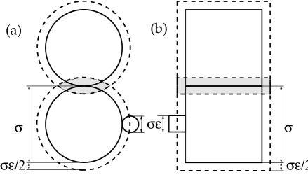
FIG. 4.: Increment in the total volume volume, $\Delta V$, available to the small particles when two large particles come to touch each other (shaded region). If $v_{0}$ denotes the volume of a large particle, $\Delta v$ is (a) $v_{0}\epsilon^{2}(3/2+\epsilon)$ for HS, and (b) $v_{0}\epsilon(1+\epsilon^{2})$, for PHC.

In other words, the depletion induced by PHC is much stronger than that induced by HS. In the infinite asymmetry limit, the binary mixture HS has been shown to reduce to the fluid of adhesive HS, provided $\eta_{2}$ is kept constant.[40] According to our estimation, in order to have a similar limit for the binary mixture of PHC we must scale the packing fraction of the small cubes as $\eta_{2}=\epsilon\xi$, with $\xi$ a constant.

We can now assume this scaling of $\eta_{2}$ and take the $\epsilon\to 0$ limit in Eq. (63). A tedious but straightforward calculation leads to

$$c_{\rm eff}({\bf r}) = c_{\rm PHC}({\bf r})+c_{\rm ad}({\bf r})\,,$$ (66)

$$c_{\rm ad}({\bf r}) = \frac{\xi}{2(1-\eta)^{2}}\left\{\delta_{\rm S}({\bf r})+yS({\bf r})+6y^{2}V({\bf r})\right\}\,,$$ (67)

where $y\equiv\eta_{1}/(1-\eta_{1})$, $c_{\rm PHC}({\bf r})$ is the DCF of the one-component PHC fluid [Eq. (56) of I], and

$$\delta_{\rm S}({\bf r}) = A(x,y,z)+A(y,z,x)+A(z,x,y)\,,$$ (68)

$$A(u,v,w) \equiv \delta(\sigma_{1}-|u|)L(v)L(w)\,,$$ (69)

$$L(u) \equiv (\sigma_{1}-|u|)\Theta(\sigma_{1}-|u|)\,,$$ (70)

$\Theta(t)$ being the usual Heaviside step function. Equation (68) represents a delta function at contact of two large cubes, multiplied by the contact surface. The functions $S({\bf r})$ and $V({\bf r})$ are the overlap surface and volume, respectively, which already appear in the definition of $c_{\rm PHC}$ [Eq. (53) of I]. In the zero density limit $c_{\rm eff}$ becomes

$$c_{\rm eff}({\bf r})\sim f({\bf r})+\xi\delta_{\rm S}({\bf r})\,,$$ (71)

with $f({\bf r})$ the Mayer function of the large cubes; so, as in HS, in the infinitely asymmetric mixture depletion induces an adhesive potential (in this case, of strength $\xi$). We will henceforth refer to this effective fluid as the fluid of parallel adhesive hard cubes (PAHC).

C Free energy functional of the fluid of parallel adhesive hard cubes

Let us now take the $\epsilon\to 0$ limit in the functional (48) to obtain the Helmholtz free-energy functional for the fluid of PAHC. In the limit we will find that $\Upsilon\to\infty$; however, this is not a problem as long as for every fixed $\epsilon$ there is a well-defined functional giving rise to a phase behaviour which do have a finite limit when $\epsilon\to 0$. We will show that this is the case, and thus this functional will be the effective functional we are looking for. We will see that the infinite contribution is just a constant shift in the origin of free energies, absolutely irrelevant for the phase behaviour.

Let us begin by recalling what FMT prescribes for the semi-grand potential (48). It is convenient to introduce two dimensionless densities, $\eta({\bf r})\equiv\sigma_{1}^{3}\rho_{1}({\bf r})$, and $\xi({\bf r})\equiv\sigma_{1}^{3}\epsilon^{2}\rho_{2}({\bf r})$. [There is no possible confusion between the function $\eta({\bf r})$ and the total packing fraction, because when $\epsilon\to 0$ the total packing fraction is simply the packing fraction of the large component, i.e. the average of $\eta({\bf r})$.] In what follows we will fix the unit length of our system by choosing $\sigma_{1}=1$. In terms of these functions the FMT form of the functional (48) is

$$\beta\Upsilon = \beta\overline{F}^{\rm id}+\int d{\bf r}\,\Phi({\bf r})$$ (73)

$$+\epsilon^{-2}\int d{\bf r}\,\xi({\bf r})\Bigl{(}\ln[{\cal V}_{2}\epsilon^{-2}\xi({\bf r})]-1-\beta\mu_{2}\Bigr{)}\,,$$

$$\beta\overline{F}^{\rm id} = \int d{\bf r}\,\eta({\bf r})\Bigl{(}\ln[{\cal V}_{1}\eta({\bf r})]-1\Bigr{)}\,.$$ (74)

Equation (74) is just the ideal Helmholtz free energy of the effective fluid, and $\Phi({\bf r})$ is given by (14), where, in the current notation, $n_{\alpha}=\eta*\omega_{1}^{(\alpha)}+\epsilon^{-2}\xi*\omega_{2}^{(\alpha)}$. But $\xi({\bf r})$ is a dependent variable which should be eliminated in terms of $\eta({\bf r})$ and $\mu_{2}$ via Eq. (49), which in our case reads

$$\ln\xi({\bf r})=\ln z-\sum_{\alpha}\frac{\partial\Phi}{\partial n_{\alpha}}*\omega^{(\alpha)}({\bf r})\,,$$ (75)

where we have defined the renormalised fugacity $z\equiv\epsilon^{2}\exp(\beta\mu_{2}^{\rm ex})$, $\mu_{2}^{\rm ex}\equiv\mu_{2}-\beta^{-1}\ln{\cal V}_{2}$. For $\xi({\bf r})$ to have a well-defined expansion in powers of $\epsilon$ we are forced to assume that $z=O(1)$.

We are almost ready to carry out the $\epsilon$-expansion. It only remains to determine the contributions to this expansion coming from convolutions with $\omega_{2}^{(\alpha)}$. Let $f(u)$ be an arbitrary function of a single variable $u$. Then

$$f*\theta^{u}_{2} = \int_{u-\epsilon/2}^{u+\epsilon/2}f(t)\,dt=\epsilon f(u)+O(\epsilon^{3})\,,$$ (76)

$$f*\delta^{u}_{2} = \frac{1}{2}[f(u+\epsilon/2)+f(u-\epsilon/2)]$$ (78)

$$=f(u)+\frac{\epsilon^{2}}{8}f^{\prime\prime}(u)+O(\epsilon^{4})\,.$$

Accordingly if $f({\bf r})$ is an arbitrary function of ${\bf r}$, from the definitions (II) and the expansions above it follows

$$f*\omega^{(0)}_{2} = f+(\epsilon^{2}/8)\nabla^{2}f+O(\epsilon^{4})\,,$$ (80)

$$f*\omega^{(\alpha)}_{2} = \epsilon^{\alpha}f+O(\epsilon^{\alpha+2})\,,$$ (81)

for $\alpha=3$ or any vector component of $\alpha=2$ and 1. Then, assuming $\xi=\xi_{0}+\xi_{1}\epsilon+\xi_{2}\epsilon^{2}+O(\epsilon^{3})$, the weighted densities $n_{\alpha}$ can be expanded as

$$n_{0} = \xi_{0}\epsilon^{-2}+\xi_{1}\epsilon^{-1}+\left\{\overline{n}_{0}+\xi_{2}+\frac{1}{8}\nabla^{2}\xi_{0}\right\}+O(\epsilon)\,,$$ (83)

$${\bf n}_{1} = \xi_{0}{\bf u}\epsilon^{-1}+\left\{\xi_{1}{\bf u}+\overline{\bf n}_{1}\right\}+O(\epsilon)\,,$$ (84)

$${\bf n}_{2} = \left\{\xi_{0}{\bf u}+\overline{\bf n}_{2}\right\}+\xi_{1}{\bf u}\epsilon+O(\epsilon^{2})\,,$$ (85)

$$n_{3} = \overline{n}_{3}+\epsilon\xi_{0}+\epsilon^{2}\xi_{1}+\epsilon^{3}\xi^{2}+O(\epsilon^{4})\,,$$ (86)

where ${\bf u}\equiv(1,1,1)$ and $\overline{n}_{\alpha}\equiv\eta*\omega_{1}^{(\alpha)}$.

 

From the expansions (V C), (V C), we can obtain

$$\sum_{\alpha}\frac{\partial\Phi}{\partial n_{\alpha}}*\omega^{(\alpha)}_{2} = -\ln(1-\overline{n}_{3})+\frac{8\xi_{0}+\overline{n}_{2}}{1-\overline{n}_{3}}\epsilon$$ (88)

$$+\left\{\frac{1}{8}\nabla\cdot\left(\frac{\nabla\overline{n}_{3}}{1-\overline{n}_{3}}\right)+\frac{1}{2}\frac{\overline{n}_{2}^{2}-\overline{\bf n}_{2}\cdot\overline{\bf n}_{2}}{(1-\overline{n}_{3})^{2}}+\frac{8\xi_{1}+\overline{n}_{1}}{1-\overline{n}_{3}}+\frac{(27/2)\xi_{0}^{2}+4\xi_{0}\overline{n}_{2}}{(1-\overline{n}_{3})^{2}}\right\}\epsilon^{2}+O(\epsilon^{3})\,.$$

On the other hand, $\ln\xi=\ln\xi_{0}+\frac{\xi_{1}}{\xi_{0}}\epsilon+\left\{\frac{\xi_{2}}{\xi_{0}}-\frac{\xi_{1}^{2}}{2\xi_{0}^{2}}\right\}\epsilon^{2}+O(\epsilon^{3})$, hence (75) implies

$$\xi_{0} = z(1-\overline{n}_{3})\,,$$ (90)

$$\xi_{1} = -z\overline{n}_{2}-8z^{2}(1-\overline{n}_{3})\,,$$ (91)

$$\xi_{2} = -\frac{z}{8}\nabla^{2}\overline{n}_{3}-z\overline{n}_{1}+12z^{2}\overline{n}_{2}+\frac{37}{2}z^{3}(1-\overline{n}_{3})-\Phi^{\rm ad}\,,$$ (92)

where for convenience we have introduced the shorthand

$$\Phi^{\rm ad}\equiv\frac{z}{8}\frac{|\nabla\overline{n}_{3}|^{2}-4\overline{\bf n}_{2}\cdot\overline{\bf n}_{2}}{1-\overline{n}_{3}}\,.$$ (93)

We have already explicitly eliminated $\xi$ in terms of $\eta$ and $z$, with the help of the expansion in $\epsilon$. We can now proceed to expand $\Upsilon$ itself, but before, let us rewrite the excess part appearing in (73) as

$$\beta\Upsilon^{\rm ex}=\epsilon^{-2}\int\xi\left[\ln\left(\frac{\xi}{z(1-\overline{n}_{3})}\right)-1\right]+\int\Bigl{\{}\Phi+\epsilon^{-2}\xi\ln(1-\overline{n}_{3})\Bigr{\}}\,;$$ (94)

then, using (V C) and (V C), and defining $\overline{\Phi}$ as in (14) with the $n_{\alpha}$ replaced by $\overline{n}_{\alpha}$ (i.e., the excess free-energy functional of the one-component PHC fluid),

$$\Phi+\epsilon^{-2}\xi\ln(1-\overline{n}_{3}) = \Bigl{\{}z\overline{n}_{2}+4z^{2}(1-\overline{n}_{3})\Bigr{\}}\epsilon^{-1}$$ (95)

$$+ \Biggl{\{}z\overline{n}_{1}-14z^{2}\overline{n}_{2}-\frac{119}{2}z^{3}(1-\overline{n}_{3})-\frac{z}{2}\frac{\overline{n}_{2}^{2}}{1-\overline{n}_{3}}+\frac{z}{8}\nabla\cdot\Bigl{[}\ln(1-\overline{n}_{3})\nabla\overline{n}_{3}\Bigr{]}+\overline{\Phi}+\Phi^{\rm ad}\Biggr{\}}+O(\epsilon)\,,$$ (96)

$$\xi\ln\left(\frac{\xi}{z(1-\overline{n}_{3})}\right)-\xi = -z(1-\overline{n}_{3})+\left\{8z^{2}\overline{n}_{2}+32z^{3}(1-\overline{n}_{3})+\frac{z}{2}\frac{\overline{n}_{2}^{2}}{1-\overline{n}_{3}}\right\}\epsilon^{2}+O(\epsilon^{3})\,.$$ (97)

 

Substituting these two expansions into (94), and using $\int\nabla\cdot[\ln(1-\overline{n}_{3})\nabla\overline{n}_{3}]=0$, which holds if the density is constant at the boundaries or if it is a periodic function, we finally obtain

$$\Upsilon=-\Pi_{0}(\epsilon)V+\mu_{0}(\epsilon)N+\overline{F}+F^{\rm ad}+O(\epsilon)\,,$$ (98)

where $\overline{F}$ is the FMT free-energy functional of the fluid of the large PHC; $V$ and $N$ are, respectively, the system volume and the number of large cubes; $F^{\rm ad}=\int\Phi^{\rm ad}$ is the new adhesive term; and $\Pi_{0}$ and $\mu_{0}$ are given by

$$\beta\Pi_{0}(\epsilon) = z\epsilon^{-2}-4z^{2}\epsilon^{-1}+\frac{55}{2}z^{3}+O(\epsilon)\,,$$ (99)

$$\beta\mu_{0}(\epsilon) = z\epsilon^{-2}+\{3z-4z^{2}\}\epsilon^{-1}$$ (101)

$$+\left\{\frac{55}{2}z^{3}-18z^{2}+3\right\}+O(\epsilon)\,.$$

The term $-\Pi_{0}(\epsilon)V+\mu_{0}(\epsilon)N$ is divergent with $\epsilon\to 0$. It is the contribution of the small cubes to the free energy (as a matter of fact, their density is infinite in this limit). However it is irrelevant for the phase behaviour of the effective fluid because it simply adds $\Pi_{0}$ to the pressure and $\mu_{0}$ to the chemical potential; as these two terms are independent of the density, they just cancel out in the equilibrium equations. Accordingly the final free energy functional for the effective one-component PAHC fluid turns out to be

$$F_{\rm PAHC}([\rho];z)=F_{\rm PHC}[\rho]+F^{\rm ad}([\rho];z)\,.$$ (102)

As a selfconsistency test, it is straightforward to show [using Eq. (90)] that $c^{\rm ad}({\bf r}-{\bf r}^{\prime})=-\beta\delta^{2}F^{\rm ad}/\delta\rho({\bf r})\delta\rho({\bf r}^{\prime})$, for the $c^{\rm ad}$ function defined in (67).

D Phase behaviour of the infinitely asymmetric binary mixture

The phase behaviour of a very asymmetric binary mixture of PHC can be understood from that of the effective fluid of PAHC, whose FMT free-energy functional we have just derived.

As concerns the phase behaviour of the uniform PAHC fluid, from (102), (14), and (93) we can readily obtain the free energy per unit volume,

$$\beta f=\eta\left\{\ln{\cal V}_{1}-1+\ln y+3(1-z/2)y+y^{2}\right\}\,.$$ (103)

The pressure, $P=-\partial F/\partial V=y^{2}\partial(f/\eta)/\partial y$, turns out to be

$$\beta P=y+3(1-z/2)y^{2}+2y^{3}\,.$$ (104)

This equation has a van der Waals loop; the critical point can be found as the solution of the equations $\partial P/\partial\eta=0$ and $\partial^{2}P/\partial\eta^{2}=0$, [45] i.e.

$$1+6(1-z_{c}/2)y_{c}+6y_{c}^{2} = 0\,,$$ (106)

$$1-z_{c}/2+2y_{c} = 0\,,$$ (107)

which is $z_{c}=2(1+\sqrt{2/3})\approx 3.63$, and $y_{c}=1/\sqrt{6}$, i.e. $\eta_{c}=1/(1+\sqrt{6})\approx 0.29$. On the other hand, the equation of the spinodal ($\partial P/\partial\eta=0$) of this vapor-liquid transition is

$$z=\frac{1+4\eta+\eta^{2}}{3\eta(1-\eta)}\,;$$ (108)

it is plotted in Fig. 5. Notice that this spinodal could have been obtained directly from (37) by taking the limit $r\to\infty$, $x\to 1$, under the constraint $r\eta(1-x)=\xi\to z(1-\eta)$ [the limit follows from (90)]. Thus it is not surprising that the line of critical points in Fig. 2 reaches $\eta_{c}$ for $x\to 1$. This makes clear the double interpretation of this transition: as a vapor-liquid transition of the PAHC fluid (with $z^{-1}$ playing the role of a temperature), or as a demixing transition of the infinitely asymmetric binary mixture.

Freezing of this system into a simple cubic lattice is again a continuous transition. Hence the transition line can be determine by the procedure described in Sec. II, i.e. as the divergence of the structure factor [Eq. (30)] with the effective DCF (66). The result is the line shown in Fig. 5. As it occurred for the general binary mixture (see Sec. III), the freezing line crosses the demixing spinodal at a packing fraction smaller than $\eta_{c}$; in other words fluid-fluid demixing is a metastable transition.

So far we have gone no further than we did in Secs. III, IV. However this time we can study fluid-solid coexistence because the density profile of the solvent is absent from the description. To proceed we again parametrise the density of the large cubes as in (II), also with a prefactor $\vartheta$ to account for vacancies. We recall that the lattice parameter is related to this occupancy ratio by $d=(\vartheta/\eta)^{1/3}$. The ideal contribution to the free energy per particle, $\Psi$, is again given by (26) (adding $\ln\vartheta$ from the vacancies), and the hard-core part of the excess contribution is given by (29) [with $n_{3}({\bf r})=\vartheta p(x)p(y)p(z)$]. We now need to work out the adhesive term. To this purpose first notice that

$$p^{\prime}(u)^{2}-q(u)^{2} = -4\sum_{n,m=-\infty}^{\infty}g(u-nd+1/2)$$ (110)

$$\times g(u-md-1/2)\,;$$

hence the adhesive free energy per particle can be written

$$\Psi^{\rm ad} = -\frac{3}{2}\vartheta z\sum_{n,m=-\infty}^{\infty}\int_{-d/2}^{d/2}dx$$ (112)

$$\times g(x-nd+1/2)g(x-md-1/2)U(x)$$

$$= -\frac{3}{2}\vartheta z\int_{-\infty}^{\infty}dx\,g(x)$$ (114)

$$\times\left[\sum_{n=-\infty}^{\infty}g(x-nd+1)\right]U(x+1/2)\,,$$

where $U(x)$ is defined as

$$U(x)\equiv\int_{-d/2}^{d/2}dy\int_{-d/2}^{d/2}dz\frac{p(y)^{2}p(z)^{2}}{1-\vartheta p(x)p(y)p(z)}\,,$$ (115)

and it is periodic with period $d$ [we have made use of periodicity in obtaining (114)].

It is convenient to rewrite Eq. (115) integrating by part with respect to both variables, $y$ and $z$; in doing so this equation becomes

$$U(x) = \int_{-d/2}^{d/2}dy\,p^{\prime}(y)\int_{-d/2}^{d/2}dz\,p^{\prime}(z)V(x,y,z)\,,$$ (116)

$$V({\bf r}) \equiv T(y)p(y)T(z)p(z)\frac{4-3n_{3}({\bf r})+3n_{3}({\bf r})^{2}}{1-n_{3}({\bf r})}\,,$$ (117)

where $T(u)=u$ if $u\in(-d/2,d/2)$ [the only relevant interval in (116)] and it is $d$-periodic. Function $V(x,y,z)$ is then also $d$-periodic in all its three arguments; accordingly Eq. (116) can be rewritten as

 

$$U(x)=\int_{-\infty}^{\infty}dy\,g(y)\int_{-\infty}^{\infty}dz\,g(z)\left[V(x,y+1/2,z+1/2)-2V(x,y+1/2,z-1/2)+V(x,y-1/2,z-1/2)\right]\,,$$ (118)

and therefore

$$\Psi^{\rm ad} = -\frac{3}{2}\vartheta z\int_{-\infty}^{\infty}dx\,g(x)\int_{-\infty}^{\infty}dy\,g(y)\int_{-\infty}^{\infty}dz\,g(z)\left[\sum_{n=-\infty}^{\infty}g(x-nd+1)\right]$$ (120)

$$\times\left[V(x+1/2,y+1/2,z+1/2)-2V(x+1/2,y+1/2,z-1/2)+V(x+1/2,y-1/2,z-1/2)\right]\,,$$

 

also suitable for Gauss-Hermite numerical integration.

In order to understand the effect of the adhesive contribution (114) let us see its asymptotic behaviour when $\alpha\to\infty$ and $d\to 1^{+}$ (equivalently $\vartheta\to\eta^{+}$), a limit which would represent a close packed solid. From its definition (16) $p(u)\sim 1$ in this limit; thus $U(x)\sim 1/(1-\eta)$. On the other hand, $g(u)$ is very sharply peaked, so

$\displaystyle\int_{-\infty}^{\infty}dx\,g(x)\sum_{n=-\infty}^{\infty}g(x-nd+1)\sim g(0)=\left(\frac{\alpha}{\pi}\right)^{1/2}\,,$

therefore

$$\Psi^{\rm ad}\sim-\frac{3}{2}z\frac{\eta}{1-\eta}\left(\frac{\alpha}{\pi}\right)^{1/2}\to-\infty\,.$$ (121)

On the other hand $\Psi^{\rm ex}=O(1)$ in this limit, while $\Psi^{\rm id}\sim 3\ln g(0)\sim(3/2)\ln\alpha$. In other words, the total free energy per particle of the effective fluid monotonically decreases as the system approaches the close packing, regardless the value of density and solvent fugacity. This means that the system always collapses, i.e. the equilibrium phase behaviour is always a close-packed solid coexisting with an infinitely diluted gas. This singular phase diagram is not exclusive of PAHC. For adhesive HS, the adhesiveness vs. packing fraction phase diagram ($z$ plays the role of adhesiveness for PAHC) has recently been mapped out from simulations of the square-well fluid in the limit of narrow and deep wells. [36] These simulations prove that the only stable phases of this system are also a close-packed solid and an infinitely diluted gas. The reason for this pathology was put forward some years ago by Stell, [46] who showed that the partition function of adhesive HS diverges if the number of particles is $N\geq 12$ (precisely the coordination number of the fcc solid lattice).

FIG. 5.: Solvent fugacity, $z$, vs. solute packing fraction, $\eta$, of the infinitely asymmetric binary mixture of PHC. The thick solid line separates the unstable region (U) from the metastable one; the thin one marks the (continuous) transition from a metastable fluid (MF) to a metastable solid (MS); the dashed one is the fluid-fluid spinodal.

In spite of the above we have seen that, as a function of $\alpha$ and $\vartheta$, the free energy per particle exhibits local minima at any value of $z$ for some range of densities, the smaller $z$ the wider this range. These local minima correspond to metastable phases. The upper bound to the packing fractions at which local minima exist for a given $z$ can be determined as the point where the compressibility vanishes. This upper bound, as a function of $z$, appears in Fig. 5. This figure shows the metastable phases. Notice that the region of metastability widens as $z$ decreases. At low $z$ these metastable phases are separated from the “collapse” by a large free energy barrier, so the system spends a long time in them before eventually becoming a close-packed solid. As a matter of fact, if the system is prepared as a metastable solid at low $z$, for a long time it will show a pseudo-coexistence between two solid phases (an expanded solid and a close-packed solid). The situation resembles the isostructural solid-solid transition reported to occur in some colloidal fluids with a narrow and deep attractive well. [36, 37] At higher $z$ the same pseudo-coexistence should be observed between a diluted fluid and a close-packed solid.

It is interesting to compare this phase behaviour with what has been determined to occur for adhesive HS using an effective-liquid DFT. [47] Fluid and solid also appear as local minima of the free energy per particle as a function of the gaussian width; however, above a certain line the free energy becomes concave up to close packing. This puzzling behaviour was interpreted in Ref. [47] as a percolation transition. In the light of our findings it is the equivalent to the instability line of Fig. 5. The fluid of adhesive HS also collapses into a close-packed solid. [36] The reason why this collapse has not been observed in Ref. [47] is that the theory used there does not account for vacancies, and this forces the lattice parameter to be larger than 1 at any packing fraction. The instability manifests itself as the reported loss of convexity of the free energy.

E Polydispersity in the large cubes

The singularity of the adhesive potential can be avoided by introducing polydispersity in the size of the particles. [46, 48] It is clear that this prevents the system to form a perfectly packed solid. To see this effect on the binary mixture we have introduced a small amount of polydispersity in the size of the large cubes. It is very easy to realise that starting off from a mixture of polydisperse large cubes and small cubes and repeating the process described in Sec. V C we end up with exactly the same form of the functional (102), with the $\overline{n}_{\alpha}$’s now replaced by those corresponding to the polydisperse mixture.

In order to make the simplest choice we consider the cubes as parallelepipeds and choose the length of each axis independently from a gaussian distribution of mean 1 and variance $\Delta\sigma$. This particular choice has two important advantages (they will be made clear below): (i) the free energy of the fluid phase is the same as that of the monodisperse system (hence its phase behaviour as well), and (ii) formally the expressions for the free energy of the solid phase change very little. It also has two drawbacks: (i) particles are not cubic anymore, and (ii) there is a nonzero contribution in the negative lengths. As these two inconvenients disappear when $\Delta\sigma\to 0$ they can be overcome by choosing $\Delta\sigma\ll 1$. This choice also allows us to make two more simplifying assumptions: (i) the ordered phase must be a substitutional solid, i.e. the density profile can be expressed as $\rho({\bf r}){\cal P}(\boldsymbol{\sigma})$, with ${\cal P}$ the normalised size distribution, $\boldsymbol{\sigma}\equiv(\sigma_{x},\sigma_{y},\sigma_{z})$, and (ii) phase separation induced by polydispersity [49] can be ignored.

Then, according to the definition of the $\overline{n}_{\alpha}$’s

$$\overline{n}_{\alpha}({\bf r})=\int d\boldsymbol{\sigma}{\cal P}(\boldsymbol{\sigma})\rho*\omega^{(\alpha)}_{\boldsymbol{\sigma}}({\bf r})=\rho*\widetilde{\omega}^{(\alpha)}({\bf r})\,,$$ (122)

i.e. it has the same definition as in the monodisperse case, but the weights are redefined as $\widetilde{\omega}^{(\alpha)}({\bf r})\equiv\int d\boldsymbol{\sigma}{\cal P}(\boldsymbol{\sigma})\omega^{(\alpha)}_{\boldsymbol{\sigma}}({\bf r})$. This amounts to replacing $\theta^{u}$ and $\delta^{u}$ in (II) by

$$\tilde{\theta}^{u} = \frac{1}{2}\left[1-\mbox{erf}\,\left(\sqrt{2}\frac{|u|-1/2}{\Delta\sigma}\right)\right]\,,$$ (124)

$$\tilde{\delta}^{u} = \frac{1}{\sqrt{2\pi}\Delta\sigma}\sum_{\{\pm\}}\exp\left\{-2\frac{(u\pm 1/2)^{2}}{\Delta\sigma^{2}}\right\}\,,$$ (125)

which are like smoothed counterparts of the original weights. Since $\int_{-\infty}^{\infty}du\,\tilde{\theta}^{u}=\int_{-\infty}^{\infty}du\,\tilde{\delta}^{u}=1$, it follows that the free energy of the uniform fluid is the same as that of the monodisperse system. Hence the fluid-fluid spinodal is the same as that shown in Fig. 5.

We can determine the coexistence between the two fluid phases by means of the usual double tangent construction. [45] Figure 6 shows the resulting coexistence line.

We can also assume a solid-like density profile as in the monodisperse case. Surprisingly enough, in spite of the striking difference of the smoothed weights defined by (V E) with respect to the original ones, when we obtain the corresponding weighted densities and work out the expressions a little bit, it turns out that the free-energy per particle of the polydisperse solid is simply given by $\Psi=\Psi^{\rm poly}+\Psi^{\rm id}+\Psi^{\rm ex}+\Psi^{\rm ad}$, where the last three contributions are given by Eqs. (26), (29), and (120), with the slight modification that the parameter $\alpha$ appearing in the definitions (5) and (15) must be replaced by

$$\widetilde{\alpha}=\frac{\alpha}{1+\alpha\Delta\sigma^{2}/2}$$ (126)

(of course, in these expressions $\sigma=1$, the mean value, and $\Psi^{\rm id}$ carries the additional $\ln\vartheta$ to account for vacancies), and where $\Psi^{\rm poly}=-\ln\left(\sqrt{2\pi}\Delta\sigma\right)-1$ is the entropy of mixing (an irrelevant constant).

From Eq. (126) it can be seen that no matter how small $\Delta\sigma$ be, for small $\alpha$’s ($\alpha\ll\Delta\sigma^{-2}$) $\widetilde{\alpha}\sim\alpha$, and the system is “blind” to polydispersity, whereas for large $\alpha$’s ($\alpha\gg\Delta\sigma^{-2}$) $\widetilde{\alpha}\sim 2\Delta\sigma^{-2}$, i.e. the system never collapses. As a consequence the singular behaviour of the monodisperse system is removed, and we can readily determine phase equilibria. A typical result for a small value of $\Delta\sigma$ is shown in Fig. 6. This figure reveals several remarkable features. Firstly, it shows that the fluid-fluid transition is metastable. Secondly, there is an isostructural solid-solid transition for a certain interval of $z$. In this interval the expanded solid (S₁) appears after a continuous transition from the fluid phase (F). The expanded solid (S₁)-dense solid (S₂) transition ends at a critical point, $z_{s}$, below which we can only find a fluid and a single solid, separated by a continuous transition. Thirdly, as $z$ increases from $z_{s}$ the expanded solid packing fraction decreases down to meeting the freezing packing fraction. Above the point where this occurs coexistence is between a fluid and a dense solid (S₂), the former quickly becoming highly diluted and the latter highly packed. Notice the strong resemblance between this true equilibrium phase behaviour and the metastable behaviour described to occur the monodisperse PAHC fluid (Sec. V D).

FIG. 6.: Same as Fig. 5 for the polydisperse PAHC fluid ($\Delta\sigma=0.045$). The thick solid line marks the fluid-solid or solid-solid coexistence; the thin one marks again the (continuous) fluid-solid transition below the coexistence region; the dotted line is the metastable fluid-fluid coexistence.

VI Discussion and conclusions

The fluid of PHC is a rather academic one which however has the great advantage of being analytically tractable in contexts where the fluid of HS is not, thanks to its adequacy to a fundamental measure description. Yet, with some peculiarities due to the lack of rotational symmetry, [10, 9] the physics it reveals is similar to that of more realistic fluids. It then allows for theoretical investigation on fluid phase behaviour otherwise very difficult (the closely related fluid of parallel hard parallelepipeds has been recently used in the context of associating fluids [50] and liquid crystals [51]). The main contribution of the fluid of PHC is to the understanding of the phase diagram of a binary mixture. This fluid proved to undergo stronger depletion than HS. [11, 12] However, as it has been shown in this work, this feature is irrelevant when the effect of depletion in the solid phase is accounted for. Spatial order of the large component strongly enhances demixing, so that fluid-solid demixing becomes the main scenario of the phase diagram of binary mixtures. But this transition can be preempted by the freezing of the large component, and when this happens the system phase separates into two fcc solids with a different lattice parameter. This effect, very clearly shown here for the mixture of PHC (in the limit of infinite asymmetry), has also been confirmed in simulations of HS interacting via an effective depletion potential, [34, 35] and very recently also in direct simulations on the true binary mixture. [38] The simulations also show that the solid-solid transition disappears as the asymmetry of the two components decreases, but it is anyhow categoric with respect to the fluid-solid nature of demixing.

A final remark concerns the two-dimensional mixture. We have made preliminary calculations in this case and have found an adhesive contribution similar to the three-dimensional one. We have nor carried out a detailed analysis yet, but the same collapse is present in this case, thus indicating a behaviour qualitatively similar to the one shown here, except that we cannot say anything on the existence of a solid-solid transition. This results are in perfect qualitative agreement with recent simulations. [52]

REFERENCES

-
[1]
E-mail:
yuri@alum.math.uc3m.es -
[2]
E-mail:
cuesta@math.uc3m.es - [3] J. A. Cuesta and Y. Martínez-Ratón, J. Chem. Phys.107, 6379 (1997).
- [4] J. A. Cuesta and Y. Martínez–Ratón, Phys. Rev. Lett.78, 3681 (1997).
- [5] R. W. Zwanzig, J. Chem. Phys.24, 855 (1956).
- [6] W. G. Hoover and A. G. de Rocco, J. Chem. Phys.36, 3141 (1962).
- [7] W. G. Hoover and J. C. Poirier, J. Chem. Phys.38, 327 (1963).
- [8] F. van Swol and L. V. Woodcock, Molec. Sim. 1, 95 (1987).
- [9] E. A. Jagla, preprint cond-mat/9807032 (1998).
- [10] T. R. Kirkpatrick, J. Chem. Phys.85, 3515 (1986).
- [11] M. Dijkstra and D. Frenkel, Phys. Rev. Lett.72, 298 (1994); M. Dijkstra, D. Frenkel and J.-P. Hansen, J. Chem. Phys.101, 3179 (1994).
- [12] J. A. Cuesta, Phys. Rev. Lett.76, 3742 (1996).
- [13] J. S. Rowlinson and F. Swinton, Liquids and Liquid Mixtures (Butterworths Scientific Publications, London, 1982).
- [14] T. W. Melnyk and B. L. Sawford, Mol. Phys. 29, 891 (1975).
- [15] D. J. Adams and I. R. McDonald, J. Chem. Phys.63, 1900 (1975).
- [16] V. Ehrenberg, H. M. Schaink, and C. Hoheisel, Physica A 169, 365 (1990).
- [17] H.-O. Carmesin, H. L. Frisch, and J. K. Percus, J. Stat. Phys. 63, 791 (1991).
- [18] J. L. Lebowitz, Phys. Rev. A133, 895 (1964).
- [19] J. L. Lebowitz and J. S. Rowlinson, J. Chem. Phys.41, 133 (1964).
- [20] T. Biben and J.-P. Hansen, Phys. Rev. Lett.66, 2215 (1991).
- [21] H. N. W. Lekkerkerker and A. Stroobants, Physica A 195, 387 (1993).
- [22] Y. Rosenfeld, Phys. Rev. Lett.72, 3831 (1994); J. Phys. Chem. 99, 2857 (1995).
- [23] J. S. van Duijneveldt, A. W. Heinen, and H. N. W. Lekkerkerker, Europhys. Lett. 21, 369 (1993).
- [24] P. D. Kaplan, J. L. Rouke, A. G. Yodh, and D. J. Pine, Phys. Rev. Lett.72, 582 (1994); A. D. Dinsmore, A. G. Yodh, and D. J. Pine, Phys. Rev. E52, 4045 (1995).
- [25] U. Steiner, A. Meller, and J. Stavans, Phys. Rev. Lett.74, 4750 (1995).
- [26] A. Imhof and J. K. G. Dhont, Phys. Rev. Lett.75, 1662 (1995).
- [27] W. C. K. Poon and P. B. Warren, Europhys. Lett. 28, 513 (1994).
- [28] C. Caccamo and G. Pellicane, Physica A 235, 149 (1997).
- [29] P. H. Fries and J.-P. Hansen, Mol. Phys. 48, 891 (1983).
- [30] G. Jackson, J. S. Rowlinson, and F. van Swol, J. Phys. Chem. 91, 4907 (1987).
- [31] A. Buhot and W. Krauth, Phys. Rev. Lett.80, 3787 (1998).
- [32] Y. Mao, M. E. Cates, and H. N. W. Lekkerkerker, Physica A 222, 10 (1995).
- [33] T. Biben, P. Bladon, and D. Frenkel, J. Phys.: Condens. Matter 8, 10799 (1996).
- [34] N. García-Almarza and E. Enciso in Proceedings of the VIII Spanish Meeting on Statistical Physics FISES ’97, edited by J. A. Cuesta and A. Sánchez (Editorial del CIEMAT, Madrid, 1998), p. 161.
- [35] M. Dijkstra, R. van Roij, and R. Evans, Phys. Rev. Lett.81, 2268 (1998).
- [36] P. Bolhuis and D. Frenkel, Phys. Rev. Lett.72, 2211 (1994); P. Bolhuis, M. Haagen, and D. Frenkel, Phys. Rev. E50, 4880 (1994).
- [37] C. F. Tejero, A. Daanoun, H. N. W. Lekkerkerker, and M. Baus, Phys. Rev. Lett.73, 752 (1994); Phys. Rev. E51, 558 (1995).
- [38] M. Dijkstra, R. van Roij, and R. Evans, preprint (1998).
- [39] T. Biben and J.-P. Hansen, Europhys. Lett. 12, 347 (1990).
- [40] Y. Heno and C. Regnaut, J. Chem. Phys.95, 9204 (1991).
- [41] Y. Martínez-Ratón and J. A. Cuesta, Phys. Rev. E(in press).
- [42] R. Evans in Inhomogeneous Fluids, edited by D. Henderson (Dekker, New York, 1992).
- [43] W. H. Press, S. A. Teukolsky, W. T. Vetterling, and B. P. Flannery, Numerical Recipes, 2nd ed. (Cambridge University Press, New York, 1992).
- [44] Notice that a FMT functional has no particular difficulties to account for vacancies in a crystal lattice, in contrast to what happens for most classical functionals. See Ref. [42] for a more detailed discussion on this matter.
- [45] H. B. Callen, Thermodynamics (Wiley, N. Y., 1960).
- [46] G. Stell, J. Stat. Phys. 63, 1203 (1991).
- [47] C. F. Tejero and M. Baus, Phys. Rev. E48, 3793 (1993).
- [48] D. Frenkel, private communication.
- [49] R. P. Sear, preprint cond-mat/9806205 (1998).
- [50] J. A. Cuesta and R. P. Sear, Euro. Phys. J. B (in press).
- [51] Y. Martínez-Ratón, J. A. Cuesta, R. van Roij, and B. Mulder in Proceedings of the NATO Advanced Study Institute “New approaches to old and new problems in liquid state theory: inhomogeneities and phase separation in simple, complex and quantum fluids”, edited by C. Caccamo, J.-P. Hansen, and G. Stell (NATO ASI Series, 1998), in press.
- [52] A. Buhot and W. Krauth, preprint cond-mat/9807014 (1998).