Spiral Surface Growth Without Desorption

Abstract

Spiral surface growth is well understood in the limit where the step motion is controlled by the local supersaturation of adatoms near the spiral ridge. In epitaxial thin-film growth, however, spirals can form in a step-flow regime where desorption of adatoms is negligible and the ridge dynamics is governed by the non-local diffusion field of adatoms on the whole surface. We investigate this limit numerically using a phase-field formulation of the Burton-Cabrera-Frank model, as well as analytically. Quantitative predictions, which differ strikingly from those of the local limit, are made for the selected step spacing as a function of the deposition flux, as well as for the dependence of the relaxation time to steady-state growth on the screw dislocation density.

Spiral surface growth is one of the most widespread growth mechanisms for crystals with atomically flat surfaces. Such crystals grow by the incorporation of new atoms at monoatomic steps. If steps are pinned at a screw dislocation, they wind around the dislocation and form growth spirals. The step dynamics, and the final steady-state spacing $l$ between successive steps (or equivalently the surface slope $a/l$, where $a$ is the lattice parameter) is determined by the interplay of surface diffusion, the attachment kinetics of atoms at the steps, and the step line tension. Recently, there has been renewed interest in spiral surface growth following the observations of spiral ridges in sputtered high-temperature superconducting thin films [1] and in certain semiconductor materials grown by molecular beam epitaxy (MBE) [2].

In the classical Burton-Cabrera-Frank (BCF) model of surface growth [3], atoms are first adsorbed to the crystalline surface (“adatoms”) and then diffuse along the surface until they are either incorporated into the crystal at a step, or desorb from the surface with a probability $1/\tau_{s}$ per unit time. Therefore, two different growth regimes can be distinguished depending on the ratio of $l$ and the diffusion length $x_{s}=\sqrt{D\tau_{s}}$, where $D$ is the surface diffusion constant. When desorption is fast ($x_{s}\ll l$), only adatoms which are deposited near a step are incorporated, and the dynamics of the steps is local, that is the velocity of a step is completely determined by the local supersaturation and the step curvature. This is the well understood regime described by the BCF theory of spiral growth [3, 4]. In many practical applications such as MBE, however, spirals can form in a step-flow regime at temperatures where desorption is negligible. Then, all deposited atoms reach a step, and successive turns of the spiral are strongly coupled via diffusion. The step dynamics becomes a highly non-local free boundary problem. The case of steady-state growth has been investigated by approximate theories [5, 6] and by the boundary integral (potential theory) method [7], but no dynamical solution of the original equations has been performed to validate these results. Another important difference between the two regimes is their approach to steady-state growth: in the local limit, the spiral finds its final step spacing essentially after a single rotation. In contrast, without desorption one would expect a slower relaxation to steady-state due to the global redistribution of adatoms. In particular, this relaxation may depend on the density of screw dislocations.

The main goal of the present letter is to use a phase-field approach to study the dynamics of spiral ridge formation in the BCF model. This approach has recently been used to efficiently solve a similar free boundary problem for dendritic growth [8], and the mathematical results of this study are exploited here. One distinguishing feature of our approach is that it makes it possible to investigate the full crossover from the local to the desorption-free limit, whereas previous works [9, 10] have assumed a constant effective supersaturation, as appropriate in the local limit. The phase field method in this context can also be interpreted as a direct continuum analog to microscopic growth models studied by Monte Carlo techniques [11]. We make quantitative predictions for the selected step spacing as a function of the deposition flux and for the time to approach steady-state growth, under the assumption that the elastic interaction between steps can be neglected. We focus mainly on the situation where adatoms feel the same barrier for attaching at ascending or descending steps, i.e. no Ehrlich-Schwoebel (ES) barrier [12], in which case attachment can be described by a single sticking coefficient $k$.

We write the BCF equations in terms of the dimensionless diffusion field $u=\Omega(c-c_{eq}^{0})$, where $c$ is the adatom concentration, $\Omega$ is the atomic area of solid, and $c_{eq}^{0}$ is the equilibrium concentration at a straight step. The basic equations have the form

$$\frac{\partial u}{\partial t}=D\,\nabla^{2}u\,-\,\frac{u}{\tau_{s}}\,+F,$$ (1)

$$v_{n}=D\left[\left(\frac{\partial u}{\partial n}\right)_{+}-\left(\frac{\partial u}{\partial n}\right)_{-}\right],$$ (2)

$$u=d_{0}\kappa,$$ (3)

where $v_{n}$ is the step normal velocity, $(\partial u/\partial n)_{\pm}$ is the normal concentration gradient on the lower $(+)$ and upper $(-)$ side of the step, $\kappa$ is the local step curvature, $d_{0}=\Omega^{2}c_{eq}^{0}\gamma/(k_{B}T)$ where $\gamma$ is the step stiffness. The effective deposition frequency $F$ is related to the actual deposition flux per atomic area $F_{d}$ by $F=F_{d}-c_{eq}\Omega/\tau_{s}$.

We simulate Eqs. 1-3 by reformulating them in terms of a phase-field model similar to the one used previously by Liu and Metiu [13] for a one-dimensional step train. The basic equations of our model are

$$\tau_{\psi}\frac{\partial\psi}{\partial t} = -\frac{\delta H}{\delta\psi}~{}=~{}W^{2}\nabla^{2}\psi\,+\,\sin\left(\pi\left[\psi-\psi_{s}\right]\right)$$ (5)

$$~{}~{}~{}~{}~{}~{}~{}~{}~{}~{}~{}~{}~{}~{}\mbox{}+\lambda\,u\left[1+\cos(\pi\left[\psi-\psi_{s}\right])\right],$$

$$\frac{\partial u}{\partial t} = D\nabla^{2}u-\frac{u}{\tau_{s}}\,+F\,-\frac{1}{2}\frac{\partial\psi}{\partial t},$$ (6)

where $H$ is the free energy functional depending on the fields $\psi$ and $u$, $\psi/2$ represents the surface height in units of $a$, $\psi_{s}/2$ is the height of the initial substrate surface, $u$ is the concentration field defined above, $W$ is the width of the step, $\tau_{\psi}$ is the characteristic time of attachment of adatoms at the steps, which is typically much smaller than $\tau_{s}$, and $\lambda$ is a dimensionless coupling constant. If we replace the coupling between the two fields in Eq. 5 by a constant supersaturation, we obtain the continuum limit of the solid-on-solid model. The main difference with the model of Ref. [13] is that the term $\left[1+\cos(\pi\left[\psi-\psi_{s}\right])\right]$ is introduced in Eq. 5 to keep the minima of $H$ at fixed values ($\psi-\psi_{s}=2n+1$), independently of the adatom concentration. A screw dislocation is introduced at the origin by choosing $\pi\psi_{s}$ equal to the polar angle in the $x$-$y$ plane, or $\pi\psi_{s}={\rm atan}(y/x)$, which corresponds to shifting the energy minima up by one atomic spacing after one complete counter-clockwise rotation.

We now use the recent asymptotic analysis of Karma and Rappel [8] to relate the equations of the phase-field model to the sharp-interface equations of the BCF model. Since the analysis of Ref. [8] applies directly to Eqs. 5 and 6, it need not be repeated here. The results of interest are that in the thin-interface limit $W/x_{s}\rightarrow 0$, the phase-field equations reduce to the free boundary problem defined by Eqs. 1 and 2, with Eq. 3 replaced by

$$u=d_{0}\kappa+v_{n}/k$$ (7)

where $d_{0}=a_{1}W/\lambda$ and $1/k=a_{1}(\tau_{\psi}/(\lambda W)-a_{2}W/D)$. The kinetic coefficient $k$ can then be made effectively infinite (instantaneous attachment), thereby recovering the condition (3) of local equilibrium, by choosing the coupling constant $\lambda=\tau_{\psi}D/(a_{2}W^{2})$. The numerical constants $a_{1}$ and $a_{2}$ are determined by the form of the energy function in Eq. 5 and can be evaluated using Eqs. 51, 54-56, and 58-59 in Ref. [8], together with the one-dimensional stationary profile solution of Eq. 5 with $u=0$ for an isolated step with $\psi(\mp\infty)=\pm 1$,

$$\psi_{0}(x)=1-\frac{4}{\pi}{\rm atan}\left(\exp\frac{\sqrt{\pi}x}{W}\right).$$ (8)

The resulting numerical values are $a_{1}=0.718348$ and $a_{2}=0.510442$. Eqs. 5 and 6 were simulated on a square lattice of edge length $L=N\Delta x$ with zero flux boundary conditions and $N$ varying between 100 and 600. As in Ref. [8], Eq. 5 was integrated using an explicit Euler scheme, Eq. 6 using a Crank-Nicholson implicit scheme. For the simulations, we measured lengths and times in units of the phase-field parameters, i. e. $W=\tau_{\psi}=1$. In these units, we chose $D=10$, which yields $\lambda=19.591$, $d_{0}=0.0366$, $\Delta x=0.5$, and $\Delta t=0.025$. The final results, stated in dimensionless ratios of physically well-defined quantities, do not depend on the choice of $W$ and $\tau_{\psi}$ as long as $W\ll x_{s}$, $W\ll l$, and $\tau_{\psi}\ll 1/F$.

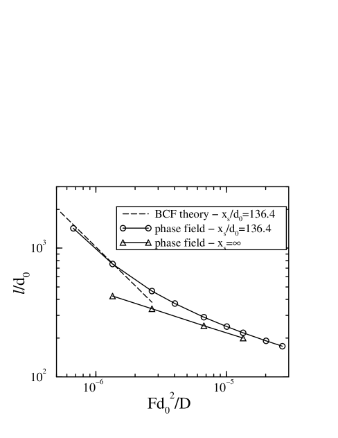
FIG. 1.: Step spacing $l$ normalized by $d_{0}$ as a function of $F$ for finite and vanishing desorption. The standard BCF theory in the local limit is shown as a dashed line for comparison.

Simulations were started from a straight ridge along the $x$-axis with one end pinned to the screw dislocation ($\psi=\psi_{s}$). After a long transient, the ridge reaches a steady-state spiral shape with a constant angular rotation frequency $\omega$, and a step spacing $l$. For our plots, we defined $l$ to be the distance between the first two successive steps from the center. This value is only a few percent smaller than the asymptotic step spacing far from the core. A plot of $l$ as a function of $F$ is shown in Fig. 1 for $x_{s}/d_{0}=136.4$, and $x_{s}=\infty$ (no desorption).

Let us now compare our results to the standard BCF theory of spiral growth that is based on the expression for the normal step velocity

$$v_{n}=v_{\infty}\left(1-r_{c}\kappa\right)$$ (9)

where $v_{\infty}$ is the velocity of a straight step and $r_{c}$ is the critical radius for island nucleation. Expressions for $\omega$ and $l$ are then obtained by looking for shape preserving solutions of Eq. 9 in a frame rotating at angular frequency $\omega$. In the local limit, $l\gg x_{s}$, the solution is [4]:

$$l = 19\,r_{c}$$ (10)

$$\omega = \frac{2\pi}{19}~{}\frac{v_{\infty}}{r_{c}},$$ (11)

with $v_{\infty}=2Fx_{s}$ and $r_{c}=d_{0}/(F\tau_{s})$; $F\tau_{s}$ is the supersaturation far away from steps. The corresponding curve for $l$ is plotted as a dashed line in Fig. 1. For an arbitrary ratio $l/x_{s}$, Eq. 9 is no longer exact because the diffusion fields of the steps overlap. Cabrera and Coleman (CC) proposed [5] that a rough estimate of $l$ and $\omega$ can be obtained by assuming that Eqs. 10-11 continue to hold with

$$v_{\infty} = 2Fx_{s}\tanh(l/2x_{s}),$$ (12)

$$r_{c} = d_{0}/u(0)=d_{0}/\left[F\tau_{s}\left(1-1/I_{0}(l/x_{s})\right)\right],$$ (13)

where Eq. 12 is the exact expression for the velocity of an infinite one-dimensional step train of spacing $l$, and $u(0)$ is the supersaturation at the center of a circular terrace of radius $l$, obtained by solving Eq. 1 subject to the boundary condition $u(l)=0$. This yields $u(r)=F\tau_{s}[1-I_{0}(r/x_{s})/I_{0}(l/x_{s})]$, where $I_{0}$ is the zero-th order modified Bessel function. One interesting consequence of the CC estimate is that in the limit $x_{s}/l\rightarrow\infty$

$$l = A(d_{0}D/F)^{1/3}$$ (14)

$$\omega = 2\pi F$$ (15)

where $A=76^{1/3}\approx 4.236$. The expression for $\omega$ is exact and follows from global mass conservation: since for $l\ll x_{s}$ all adatoms reach a step, the spiral rotation frequency must just be $F$ in steady-state. The same scaling relations, but with a different prefactor $A$ have been obtained by the boundary integral method [7]. The scaling for $l$ becomes exact in the limit $d_{0}/l\rightarrow 0$, which is practically always satisfied. This can be understood from a simple dimensional analysis. In the limit where $\tau_{s}\rightarrow\infty$, all parameters can be removed from the BCF equations by making the variable transformations

$$t^{\prime}=tF,~{}x^{\prime}=x(F/d_{0}D)^{1/3},~{}u^{\prime}=u(D/d_{0}^{2}F)^{1/3},$$ (16)

if one neglects $\partial_{t}u$ in Eq. 1 which is of relative magnitude $d_{0}/l$. Our numerical results confirm this scaling and yield a value of $A=4.626$. They also show that the cross-over from $l\sim F^{-1}$ to $l\sim F^{-1/3}$ is very slow.

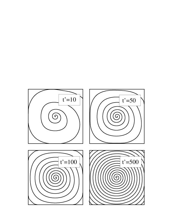
FIG. 2.: Spiral ridge at different times $t^{\prime}=tF$, equivalent to the number of monolayers deposited, for $x_{s}=\infty$, $Fd_{0}^{2}/D=1.344\times 10^{-5}$, and $L/d_{0}=5464$.

Next, let us examine how the dynamical aspects of the spiral ridge formation depend on the system size $L$, which on a real surface is roughly given by the mean distance between dislocations. In the local limit $x_{s}\ll l$, $\omega$ and $l$ are sharply selected on a time scale of one rotation, and the ridge winds itself into a classic Archimedian spiral (i.e. spiral with a constant $l$) in $\sim L/l$ rotations. In contrast, Fig. 2 shows that, in the desorption-free limit, the transient spiral ridge evolves extremely slowly towards an Archimedian spiral via a progressive reduction of the step spacing away from the core. The rotation frequency of the center is faster than $F$ at the beginning, as a larger step spacing allows more adatoms to attach to the ridge, and then slowly approaches $F$. In addition, Fig. 2 shows that the shape is strongly influenced by the boundaries during the initial transient. The final spacing, however, is independent of the system size. In order to quantify the transient dynamics, we calculate the surface width

$$w(t)=\frac{1}{2}<\psi(x,t)^{2}-<\psi(x,t)>^{2}>^{1/2}$$ (17)

where $<f>\equiv L^{-2}\int fdxdy$. In steady-state, we simply have $w(t\rightarrow\infty)\propto L/l$ for $L\gg l$. We plot in Fig. 3 $w(t)/(L/l)$ as a function of $Ft/(L/l)^{3}$ for different system sizes. The data collapse remarkably onto a single curve, which shows that the time to reach steady state scales as $(L/l)^{3}$. This cubic law can be understood analytically by considering the train dynamics in the region away from the spiral core. In this region, the effect of the step curvature can be neglected and a one-dimensional step train is governed by the simple evolution equation $\partial_{t}l_{n}=(F/2)(l_{n-1}-l_{n+1})$, where $l_{n}$ is the distance between the $n$th and $n+1$th steps.

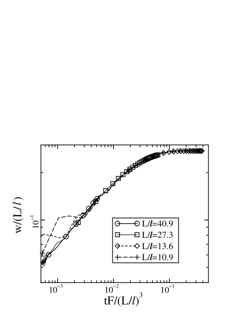
FIG. 3.: Rescaled surface width $w/(L/l)$ as a function of rescaled time $tF/(L/l)^{3}$ for four different system sizes. The large fluctuations at early times occur during the initial winding of the straight ridge into a spiral shape.

This set of discrete equations can be transformed into a continuum equation for the coarse-grained surface height $h(x,t)$ (in units of $a$) of the standard conserved form [14]:

$$\partial_{t}h=F-\partial_{x}J,$$ (18)

where $J$ is the surface current. Here, $J=-D\partial_{x}<u>$ where $<u>=Fl^{2}/12D=F/12D(\partial_{x}h)^{2}$ is the the average adatom concentration between two steps, which combined with Eq. 18 yields

$$\partial_{t}h=F+\frac{F}{12}\,\partial_{x}^{2}\left(\frac{1}{(\partial_{x}h)^{2}}\right).$$ (19)

This equation has a scaling solution of the form

$$h(x,t)=Ft+(L/l)\tilde{h}(x/(L/l),tF/(L/l)^{3}),$$ (20)

where the system size drops out of the resulting equation for $\tilde{h}$. Thus, the relaxation time depends on the third power of the system size as observed in our simulations.

Let us now examine how these results become modified when the assumption of local equilibrium at the step is relaxed by letting $k$ be finite in Eq. 7. In this case, an approximate expression for $l$ can be obtained by repeating the estimate of CC with the modified boundary condition $u(l)=v_{\infty}/k=Fl/k$ at the edge of the circular terrace around the dislocation center. This yields $u(0)=(1+4D/lk)Fl^{2}/4D$, where as before $l=19d_{0}/u(0)$. So for fast attachment ($4D/lk\ll 1$) we recover the previous scaling $l\sim F^{-1/3}$, whereas for slow attachment ($4D/lk\gg 1$) we obtain the scaling $l\sim(d_{0}k/F)^{1/2}$ in agreement with boundary integral results [7]. We performed a series of simulations with a finite $k$ by choosing $\lambda=1$ and observed a slow cross-over towards $F^{-1/2}$ with increasing $F$, which is consistent with this prediction. The spiral ridge was also found to relax much slower than in the local limit but we did not conduct a systematic finite size scaling analysis to determine the dependence on $L$. Finally, if the present analyses are extended to the case of a finite ES barrier, one concludes that the scaling $l\sim F^{-1/3}$ remains unchanged. In this case, however, the step train away from the spiral core is known to be morphologically unstable [15], and this instability may alter spiral growth in ways that remain to be investigated.

Several of the present predictions should be experimentally testable. If desorption is negligible, one should observe a dependence of the form $l\sim F^{-\alpha}$ with $\alpha$ between $1/3$ and $1/2$. Moreover, by examining the ridge dynamics one can obtain information about the relative importance of desorption and diffusion. In particular, in experiments the distance $L$ between screw dislocation centers is often in the range of five to ten $l$ [1, 2]. If desorption is negligible, the cubic dependence of the relaxation time to steady-state growth on $l$ implies that the spiral ridge should reach a maximum surface slope only after a few hundred monolayers are deposited.

The present phase-field approach should be generally applicable to simulate a wide range of mesoscopic surface growth phenomena. Interesting future prospects are to include concentration fluctuations to study the crossover from spiral growth to island nucleation at high temperature/flux, to study the effect of anisotropy of the line tension and/or the attachment kinetics on the growth morphology, and to include an ES barrier. Finally, elastic effects which have recently been shown to influence spiral growth dynamics [10] could be incorporated by coupling the dynamics of $\psi$ and $u$ to the strain field.

This research was supported by US DOE grant No DE-FG02-92ER45471 and benefited from supercomputer time at NERSC. We thank R. Kohn, D. Wolf, and A. Zangwill for valuable exchanges.

REFERENCES

- [1] M. Hawley, I. D. Raistrick, J. G. Beery, and R. J.Houlton, Science 251, 1587 (1991); C. Gerber, D. Anselmatti, J. G. Bednorz, J. Mannhart, and D. G. Schlom, Nature 350, 279 (1991).
- [2] G. Springholz, A. Y. Ueta, N. Frank, and G. Bauer, Appl. Phys. Lett. 69, 2822 (1996).
- [3] W. K. Burton, N. Cabrera, and F. C. Frank, Philos. Trans. R. Soc. London, Ser. A243, 299 (1951).
- [4] N. Cabrera and M. M. Levine, Phil. Mag. 1, 450 (1956).
- [5] N. Cabrera and R. V. Coleman, in: The Art and Science of Growing Crystals, ed. by J. J. Gilman, John Wiley, New York (1963).
- [6] T. Surek, J. P. Hirth, and G. M. Pound, J. Cryst. Growth 18, 20 (1973).
- [7] J. P. van der Eerden, J. Cryst. Growth 53, 305, 315 (1981); see also J. P. van der Eerden, in Handbook of Crystal Growth, Vol. 1a, ed. by D. T. J. Hurle, Elsevier (1993).
- [8] A. Karma and W.-J. Rappel, Phys. Rev. Lett 77, 4050 (1996); Phys. Rev. E 57, 4323 (1998).
- [9] F. Falo, A. R. Bishop, P. S. Lomdahl, and B. Horovitz, Phys. Rev. B 43, 8081 (1991).
- [10] I. S. Aranson, A. R. Bishop, I. Daruka, and V. M. Vinokur, Phys. Rev. Lett. 80, 1770 (1998).
- [11] R. H. Swendsen, P. J. Kortman, D. P. Landau, and H. Müller-Krumbhaar, J. Cryst. Growth 35, 73 (1976); R.-F. Xiao, J. I. D. Alexander, and F. Rosenberger, J. Cryst. Growth 109, 43 (1991).
- [12] G. Ehrlich and F.G. Hudda, J. Chem. Phys. 44, 1039 (1966); R.L. Schwoebel and E.J. Shipsey, J. Appl. Phys. 37, 3682 (1966).
- [13] F. Liu, H. Metiu, Phys. Rev. E 49, 2601 (1994).
- [14] J. Villain, J. Phys. I (France) 1, 19 (1991)
- [15] G. S. Bales and A. Zangwill, Phys. Rev. B 41, 5500 (1990).