Filling a Silo with a Mixture of Grains:
Friction-Induced Segregation

Abstract

We study the filling process of a two-dimensional silo with inelastic particles by simulation of a granular media lattice gas (GMLG) model. We calculate the surface shape and flow profiles for a monodisperse system and we introduce a novel generalization of the GMLG model for a binary mixture of particles of different friction properties where, for the first time, we measure the segregation process on the surface. The results are in good agreement with a recent theory, and we explain the observed small deviations by the nonuniform velocity profile.

Mixtures of grains tend to separate as a response to virtually any type of external perturbation [1], an effect that can be a major problem in some practical situations, and useful in others. Indeed, understanding the underlying processes of segregation phenomena in granular mixtures is an intriguing problem of interest to scientists from a wide range of disciplines.

Segregation occurs when a mixture is poured onto a horizontal base and a pile builds up. When the grains of the mixture differ in size, the large grains tend to gather at the bottom of the pile [2], while when the grains have different shapes, the more faceted grains are found preferentially near the top. An even more surprising effect can be observed when a mixture of small rounded and large faceted grains is poured between two parallel plates: Stratification is observed—i.e., the grains organize spontaneously into stripes [3].

Particle size distribution crucially influences segregation. However, the particles generally differ not only in size but also in other properties, such as frictional ones. Frictional effects play a relevant role in band formation in 3-D rotating drums, in segregation in thin rotating drums, and also segregation and stratification in 2-D silos. Thus the study of the particular case where segregation is caused solely by differences in friction coefficients tells the contribution of friction to these segregation processes.

The description of segregation in the case of a bidisperse pile is nontrivial. A theory was proposed for the two-dimensional case [4], which is a generalization of a method developed [5] for avalanches in piles of monodisperse particles that treats the static bulk and the fluidized surface (the rolling phase) separately, and a set of continuum equations describes the dynamics of the flowing region and the interactions between the two phases. Solutions have been found for the steady state filling of a 2D silo for the case of monodisperse particles. The theory provides also predictions for the surface and segregation profiles in a binary mixture consisting of grains with different friction properties but the same size [4].

It is important to test these theoretical predictions for two reasons. First, the complete description requires a number of constitutive relations between the relevant variables of the problem; these are usually unknown and are assumed to have analytically treatable functional forms, which should be verified. Second, in order to derive closed formulae for the profiles, several assumptions are made, so the limits of these approximations are of interest. Hence we have carried out a program of computer simulations using the granular media lattice gas (GMLG) model, which has been used for several granular systems, such as pipe flows, shaken boxes, and static piles [6, 7, 8]. An advantage of the simulation approach is that quantities can be measured that are inaccessible in laboratory experiments.

In the GMLG model[6], one generalizes a fully discrete hydrodynamic algorithm [9] in order to include energy dissipation through particle collisions and friction. The indistinguishable point-like particles are either at rest or else they travel with unit momentum along the bonds of a triangular lattice. The particles are scattered at the lattice nodes at integer times and then they are transferred to the nearest-neighbor sites in parallel.

We adapt the GMLG algorithm to the case of two types of particles with different friction properties, which we call up and down particles [4]. Using probability variables, we introduce material parameters in a stochastic way. The restitution coefficient is described by a parameter $\varepsilon$, which is the probability that energy is conserved in a collision (an example of the application of this rule is shown in Fig. 1a). Momentum is conserved if the particles in a collision are not connected, even in an indirect way, to the wall.

The compact static part of the pile behaves like a solid with a large mass, where friction effects are taken into account. When moving particles interact with the bulk, their momentum can be transferred through the force chains to the walls of the vessel. For two types of grains, we define four different friction coefficients $\mu_{\alpha\beta},$ $(\alpha,\beta\in\uparrow,\downarrow)$, giving the probability of a moving particle of type $\alpha$ to stop when arriving at a bulk site containing a particle of type $\beta$ (Fig. 1b). Bulk particles are rest particles that are supported by another bulk particle or by the vessel. The particles have equal size, their distinction being introduced through different friction coefficients [4].

We study the steady state filling process of a two-dimensional “silo”, i.e., a long rectangular box of lateral size $L$. The silo is filled with a steady flux of particles $Q$ next to the right wall. Two typical snapshots are shown in Fig. 2 for a monodisperse system of particles and for a binary mixture. The theory focuses on the limit of very slow, but still continuous filling. In general, the steady state slope depends on the incoming particle flux but this dependence vanishes at low rates. We find that for $Q\leq 0.5{{\rm particle\over update~{}step}}$, the slope will indeed be independent of the filling rate, while we still observe smooth and non-intermittent growth. For even smaller incoming flux ($Q<0.1$ in the above units) the pile grows intermittently. This avalanche regime was studied in Ref. [6] in detail.

In steady filling of a monodisperse species, theory predicts that the thickness of the rolling particle layer, $R(x)$, decreases linearly down the slope[4], and that the local slope $\theta(x)$ is close to the angle of repose $\theta_{rep}$ everywhere but near the bottom of the pile (see also Ref. [8] for the case of a sandpile in an open cell),

$$R(x)={Q\over vL}x,\qquad\qquad\displaystyle{\theta(x)=\theta_{rep}-{v\over\gamma x}}.$$ (1)

Here $\gamma$ describes the rate of exchange between the bulk and the rolling phase, and $v/\gamma$ is of the order of the grain size. We assume the flow velocity $v$ to be constant in space and time.

Next we test these predictions by calculating $R(x)$, defined in the simulation by the average number of rolling particles at each $x$, and the height of the pile, $\partial h(x)/\partial x\equiv\tan\theta(x)$. We take data when the steady state is reached, and we repeat the measurements at time intervals during which the pile grows about two lattice sites in height. We average the data over an ensemble of $10-100$ systems. The number of particles at the end of each run is typically of the order of $10^{5}$.

Figure 3 shows the simulated profiles for the monodisperse case. Figure 3a illustrates the fact that [see Eq. (1)]

$$R(x)\propto x$$ (2)

with reasonable precision. The slight deviation from linearity can be understood due to corrections to the velocity profile. Equation (2) comes from a conservation of grains argument, assuming that the velocity of the rolling grains $v$ is constant along the slope. However, at the bottom, where the slope is less steep we expect the particles to slow down and this is also observed in the simulations. If we take this into account theoretically by introducing a first-order correction to the velocity, $v(\theta)=v_{0}+\lambda(\theta-\theta_{rep})$, we arrive at an implicit formula for $R(x)$ (solutions for $\lambda=0$ were derived in Ref.[4]):

$$R_{t}(x)\equiv R(x)+{{\lambda Q}\over{v_{0}L\gamma}}\ln\left(R(x){v_{0}\over Q}\right)={Q\over{v_{0}L}}x.$$ (3)

By transforming our data with this solution, we obtain an excellent fit (Fig. 3a inset).

From the height profile (Fig. 3), we see that the slope at the upper part is almost constant, and a region can be found at the bottom where the surface flattens out. The singularity at $x=0$ [Eq. (1)] cannot be seen, since both in real systems and in simulations there is a cutoff due to the grain size, but the profile does bend up (for small $\varepsilon$) near $x=0$. This effect has also been observed experimentally [10]. The singularity can be avoided by re-defining the interaction term between the rolling and static grains.

If the silo is filled with a mixture of particles (Fig. 2b), the growth process is considerably more complicated. In general, instead of one single angle of repose there are two continuous sets of generalized angles of repose for the two species [3] – denoted by $\theta_{\uparrow}$ and $\theta_{\downarrow}$ – since the local critical angles depend also on the volume fraction of the species in the bulk. The curves are characterized by four variables $\theta_{\alpha\beta}$, which are the critical angles for particles of type $\alpha$ rolling on a pure static phase consisting of grain type $\beta$. As in Ref. [4], we assume that both curves are constant. Then the number of critical angles reduces to two constants $\theta_{\uparrow}=\theta_{\uparrow\uparrow}=\theta_{\uparrow\downarrow}$ and $\theta_{\downarrow}=\theta_{\downarrow\downarrow}=\theta_{\downarrow\uparrow}$ (or equivalently, $\mu_{\uparrow}$ and $\mu_{\downarrow}$) [3].

The rolling phase in the steady state is described by the number of rolling particles for each species $R_{\alpha}(x)$ (with $\alpha\in\uparrow,\downarrow$), and the static phase by the bulk volume fractions $\Phi_{\uparrow}(x)$, and $\Phi_{\downarrow}(x)$, where $\Phi_{\uparrow}+\Phi_{\downarrow}=1$. We distinguish two regions, where different analytic results have been obtained [4]. The outer region includes almost the entire pile surface except for a narrow zone, the inner region, close to the bottom of the pile. We will focus on the flow properties in the outer region. The profile $R(x)\equiv R_{\uparrow}(x)+R_{\downarrow}(x)$ is given by Eq. (1) while the profiles of the components can be expressed in terms of an exponent $r$:

$$R_{\uparrow}(x)={R(x)\over{1+{Q_{\downarrow}\over Q_{\uparrow}}\bigl{(}{L\over x}\bigr{)}^{r}}},$$ (4)

$$R_{\downarrow}(x)={R(x)\over{1+{Q_{\uparrow}\over Q_{\downarrow}}\bigl{(}{x\over L}\bigr{)}^{r}}}.$$ (5)

The exponent $r$ plays also a role in the determination of the bulk volume fractions $\Phi_{\uparrow}$ and $\Phi_{\downarrow}$:

$$\Phi_{\uparrow}(x)=\biggl{(}1+r{R_{\downarrow}(x)\over R(x)}\biggr{)}{R_{\uparrow}(x)\over R(x)},$$ (6)

$$\Phi_{\downarrow}(x)=\biggl{(}1-r{R_{\uparrow}(x)\over R(x)}\biggr{)}{R_{\downarrow}(x)\over R(x)}$$ (7)

Here we assume a homogeneous rolling phase with constant velocity $v\equiv v_{\uparrow}=v_{\downarrow}$, and $Q_{\uparrow}$ and $Q_{\downarrow}$ are the fluxes of each species. The exponent $r$ depends on the structure of the collision matrix describing the interaction between the bulk and rolling phase.

To analyze the simulation data, we calculate the exponent $r$ from the measured $R(x)$ and $R_{\alpha}(x)$ profiles for all $x$. The most significant test of the theory is the existence of $r$; if $r$ is well-defined, the volume fraction profiles can be calculated and compared to the measured ones.

Figure 2b shows a snapshot of the simulation for a mixture with $\mu_{\uparrow}=0.25$ ($\theta_{\uparrow}=57^{\rm o}$) and $\mu_{\downarrow}=0.152$ ($\theta_{\downarrow}=48^{\rm o}$). We see the segregation of the mixture with the more sticky species ($\uparrow$) at the top of the pile. Figure 4a shows typical moving particle profiles. It is apparent that there is a slight higher order deviation from linearity in the case of $R(x)$, as opposed to the prediction of Eq. (2). The discrepancy is small, but it is significant enough that the theoretical profiles based on a linear approximation of the curve do not fit the simulation results. However, if we use the measured $R(x)$ for calculating the rolling particle profiles, Eqs. (4) and (5) hold to a better approximation (this bias will be discussed below).

Most crucial is to verify Eqs. (4) and (5) by calculating $r$. We present results for two sets of critical angles $A$ and $B$, with $\psi_{A}\approx 0.15$ and $\psi_{B}\approx 0.5$, where $\psi\equiv\theta_{\uparrow}-\theta_{\downarrow}$. Figure 5 demonstrates that the exponent is well defined in both cases except for a region at the top of the pile. The measured exponents are $r_{A}=0.19\pm 0.02$ and $r_{B}=0.51\pm 0.03$. This result is reassuring since $r$ is expected to be of the order of $\psi$  [4]. The exponent slightly depends on the $Q_{\downarrow}/Q_{\uparrow}$ ratio, but is independent of the total flux provided $Q$ is sufficiently small.

With the help of the exponent we can obtain the volume fraction profiles based on Eqs. (6) and (7), and compare them to the measured ones (Fig. 4b). We find good agreement, except for a slight deviation in the inner region. We find stronger segregation for larger $\psi$ (or $r$); for the small angle difference $\psi_{A}$ the segregation of the species is less pronounced.

Although the numerical results fit the continuum theory, we observe some deviations. At the top of the pile, we see a discrepancy both at the rolling particle profiles and when calculating the $r$ exponent. Here the dynamics is significantly different from what is considered in the continuum model: moving particles tend to be in free flight after collisions with the pile surface.

Relation (2) is not satisfied rigorously, as mentioned above. The reason is that, similar to the monodisperse case, the $x$ component of the velocity is not uniform. For a weighted sum of the rolling particle densities, however, linearity should hold to a better approximation: $v_{\uparrow}(x)R_{\uparrow}(x)+v_{\downarrow}(x)R_{\downarrow}(x)\propto x$. We show a justification of this ansatz in Fig. 4a, by using the measured $v_{\uparrow}(x)$ and $v_{\downarrow}(x)$ functions. The functional forms of these profiles can be approximated by $v_{0}-{a\over x}$, where $v_{0}=0.9\pm 0.01{\rm lattice~{}unit\over update~{}step}$ and $a=1.6\pm 0.2{\rm lattice~{}unit^{2}\over update~{}step}$ are fitting parameters. The functional form of the velocities is consistent with the correction we found for the monodisperse system $v_{\alpha}(x)=v_{0}+\lambda(\theta-\theta_{\alpha})$, $\alpha\in\uparrow,\downarrow$, assuming that the angle of the pile behaves approximately as Eq. (1).

In general, we expect deviations from the theoretical predictions as an increasing number of particles are in free flight above the pile. If many particles tend to get detached from the surface due to elastic collisions such a contribution should also be incorporated into the theory. In the numerical results presented above, both particle-particle and particle-wall collisions are almost perfectly inelastic (the coefficient of restitution is around $0.25$). Test runs for a more elastic medium show that the exponent describing the $R_{\alpha}(x)$ profiles is no longer constant as a function of $x$ indicating the limits of the theory.

In summary, we have simulated the filling process of a two-dimensional silo, and our results for inelastic particles compare well with the predictions of recent theories of surface flow of granular mixtures. We find small corrections that are accounted for by a modified set of equations. Thus, we have verified the main assumptions of the theory, pointed out the limits of the approximations involved, suggested improvements, and found good agreement between the simulation results and the improved theory. Future work is needed to test further the limitations of the theory and to generalize the model to more complex situations like polydispersity in the particle size distribution.

This work was supported by OTKA (T016568, T024004), MAKA (93b-352), the Heinrich-Hertz Stiftung, and the NSF.

FIG.1 (a) Illustration of the implementation of the restitution coefficient through a triple collision. If energy is conserved—with probability $\varepsilon$—the particles are scattered. If the collision is dissipative—with probability ($1-\varepsilon$)—the particles stop. (b) An example of the application of the friction rule, when a moving particle of type $\alpha$ (white) arrives at a bulk site with a particle of type $\beta$ (shadow). With probability $\mu_{\alpha\beta}$, the particle of type $\alpha$ loses its energy and becomes part of the bulk, while with probability $1-\mu_{\alpha\beta}$ its momentum is conserved and the node is not considered to belong any longer to the static phase.

FIG.2 Two simulation snapshots for the steady filling of a silo, which is being filled with (a) uniform particles (b) a mixture of two different types of particles. Note that each pixel represents a lattice node that can be occupied by up to six particles. In (b) black and white dots denote lattice nodes where the $\downarrow$ and $\uparrow$ particles are in majority, respectively ($\theta_{\uparrow}>\theta_{\downarrow}$). The more sticky $\uparrow$ particles are found preferentially at the top.

FIG.3 Profiles of the growing pile in the steady state of the monodisperse system. (a) The average number of rolling particles, $R(x)$. The inset shows that $R_{t}(x)$ [see Eq. (3)] is indeed proportional to $x$ to a good approximation, with fitting parameter $\lambda=0.1{\rm lattice~{}unit\over update~{}step}$. (b) The height of the surface, $h(x)$. At each measurement the mean height is subtracted, since the pile is constantly growing. On Figs.3-5 quantities are given in natural units of the simulation method: Lengths are measured in lattice constants, times in update steps.

FIG.4 Profiles in case of a granular mixture for $\psi_{B}\approx 0.5$. (a) Rolling particles. The continuous lines are fits calculated using Eqs. (4) and (5). The inset shows that $v_{\uparrow}R_{\uparrow}+v_{\downarrow}R_{\downarrow}\propto x$. (b) Volume fraction of the $\downarrow$ particles in the static bulk. (For the $\uparrow$ particles $\Phi_{\uparrow}=1-\Phi_{\downarrow}$.) The continuous line shows the calculated profile according to Eq. (7) using the measured $r$ exponent.

FIG.5 The value of the exponent $r$ calculated at each site $x$ for $\psi_{A}=0.15$ and $\psi_{B}=0.5$; $r$ is well-defined except for the uppermost part of the pile.

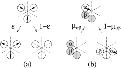
FIG. 1.:

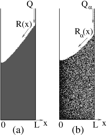
FIG. 2.:

FIG. 3.:

FIG. 4.:

FIG. 5.:

REFERENCES

- [1] See, e.g., the recent book Physics of Dry Granular Matter, edited by H. J. Herrmann and R. P. Behringer (Kluwer, Dordrecht, 1998), and extensive references therein.
- [2] R. L. Brown, J. Inst. Fuel 13, 15 (1939).
- [3] See H. A. Makse, P. Cizeau, and H. E. Stanley, Phys. Rev. Lett. 78, 3298 (1997) and references therein.
- [4] T. Boutreux and P.G. de Gennes, J. Phys. I 6, 1295 (1996).
- [5] J.P. Bouchaud et al, Phys. Rev. Lett. 74, 1982 (1995).
- [6] J. Kertész and A. Károlyi, in Proc. 6th EPS-APS Intl. Conf. on Physics Computing (EPS, Geneva, 1994); A. Károlyi and J. Kertész, Phys. Rev. E 57, 852 (1998).
- [7] G. Peng and H. J. Herrmann, Phys. Rev. E 49, R1796 (1994); S. Vollmar and H. J. Herrmann, Physica A 215, 411 (1995).
- [8] J.J. Alonso and H. J. Herrmann, Phys. Rev. Lett. 76, 4911 (1996).
- [9] U. Frisch, B. Hasslacher and Y. Pomeau, Phys. Rev. Lett. 56, 1505 (1986); G. D. Doolen, Editor, Lattice Gas Methods for Partial Differential Equations, (Addison Wesley, 1990).
- [10] Y. Grasselli and H. J. Herrmann, Comptes Rendus de l’Acad. des Sci. Paris, t.325, Série IIb, in press.