The Hartree approximation in dynamics of polymeric manifolds in the melt

Abstract

The Martin-Siggia-Rose (MSR) functional integral technique is applied to the dynamics of a D - dimensional manifold in a melt of similar manifolds. The integration over the collective variables of the melt can be simply implemented in the framework of the dynamical random phase approximation (RPA). The resulting effective action functional of the test manifold is treated by making use of the selfconsistent Hartree approximation. As an outcome the generalized Rouse equation (GRE) of the test manifold is derived and its static and dynamic properties are studied. It was found that the static upper critical dimension, $d_{\rm uc}=2D/(2-D)$, discriminates between Gaussian (or screened) and non-Gaussian regimes, whereas its dynamical counterpart, ${\tilde{d}}_{uc}=2d_{\rm uc}$, distinguishes between the simple Rouse and the renormalized Rouse behavior. We have argued that the Rouse mode correlation function has a stretched exponential form. The subdiffusional exponents for this regime are calculated explicitly. The special case of linear chains, $D=1$, shows good agreement with Monte-Carlo-simulations (MC).

I Introduction

There has been recent interest in the dynamical behavior of polymers (or more generally polymeric manifolds) in a quenched disordered random medium [1, 2] and in a melt [3, 4, 5, 6, 7, 8]. The dynamics of flux-lines in a type II superconductor [9] also belongs to the same class of problems as in [1, 2]. The derivation of the equations of motion for the time correlation functions has been carried out by making use either of the projection formalism and the mode-coupling approximation [3, 4, 5, 6, 7] or the Martin-Siggia-Rose (MSR) functional technique and the selfconsistent Hartree approximation [1, 8, 9]. The latter theoretical approach (which is equivalent to the Hartree type approximation) was earlier also successfully applied to the investigation of static properties of different models with [10, 11, 12] or without [13, 14, 15] replica symmetry breaking.

The basic description for polymer dynamics in general is the so-called Rouse model [16, 17], where the polymer configuration is expressed in dynamical modes. The physical background of the Rouse model is very simple: It corresponds to a non interacting chain stirred by a white noise random force, in the usual Langevin sense. It is well known from experiments [18], but also very surprising that this Rouse model provides a good description for the melt of the relatively short chains $N<N_{e}$. At higher degrees of polymerization the dynamics of the long chain can be described by the reptation model [16, 17, 19]. For the case of the short chain melt, it is not obvious that the collisions of the surrounding chains close to a test chain add up to a white noise force. On the other hand, the obvious thought to explain the Rouseian behavior in short chain polymer melts is first the excluded volume screening and second the inactivity of topological constraints (”entanglements”) at these length scales. The chain in a melt has Gaussian statistics, i.e., $R\propto\sqrt{N}$ can be explained by the screening of the excluded volume interactions [16, 17]. In this case the chains (or generally speaking polymeric manifolds) strongly interpenetrate. The screening of exclude volume reduces the upper critical dimension of the interactions (from four to approximately two in the case of linear chains), and we can expect that for higher connected polymers such as $D$ - dimensional manifolds the screening becomes also dependent upon the embedding space dimension $d$ and the connectivity.

Nevertheless we show below in this paper that in the case of dynamics the situation is more complicated, even for linear chains. The screening of the excluded volume interactions leads by no means automatically to the Rouse dynamics even for the short chains. Indeed we will show that the interactions introduce a new dynamical regime in $2\leq d\leq 4$. This new regime is derived on different grounds than those proposed by Schweizer [4, 5]. Moreover we need to resolve the following questions: How does the bare monomeric friction coefficient $\xi_{0}$ renormalize due to the interactions of the test chain with the surrounding melt? Under which conditions is renormalization relevant? A short presentation of the results of this paper was given in a recent letter [21].

We use here the MSR-functional technique and the selfconsistent Hartree approximation for the investigation of the static and mainly dynamic properties of a polymeric $D$ - dimensional manifold [22] (or a fractal) in the melt of the same species. One of the main results of the present study is the derivation of a generalized Rouse equation (GRE) for such D-dimensional manifold. In this equation the static and dynamic parts are treated on a equal footing and in the static limit the screening and saturation of $D$ - dimensional manifolds are reproduced in a different way than in [23].

We should stress that the manifolds in our consideration have phantom springs, i.e. are crossable, so that entanglements cannot occur and the reptational dynamics is not considered here. The reptational dynamics is driven by topological constraints and will be considered in a subsequent publication. We describe below the manifolds only in terms of connectivity and excluded volume interactions. The connectivity defines the $D$ - dimensional subspace which is embedded in the Euclidean space of $d$ dimensions.

This model includes the cases between linear polymer chains, which correspond to $D=1$, and tethered membranes (D=2). By analytic continuation to rational numbers of the spectral dimension statements on polymeric fractals can be made. Branched polymers (and percolation clusters) correspond closely to the spectral dimension $D=4/3$. In a series of papers [23] one of us has considered the different regimes in static scaling. Here we will find that these regimes besides the Gaussian one are unstable. Nevertheless we will show below that a new dynamical regime for the motion of manifold segments appears. The whole dynamical consideration results in a sub-diffusive behavior and exponents, which are confirmed for a melt of linear chains in 3 - dimensions by Monte-Carlo (MC) numerical investigations [24, 25, 26, 27, 28] (see also [29, 30, 31]).

The paper is organized as follows. In Sec. II, we define the system and derive the GRE. To do this we integrate over the matrix collective variables. The resulting action in terms of the test manifold variables will be treated in the framework of the Hartree approximation. In Sec. III, on the basis of the GRE the static and dynamic properties of the test manifold in the melt are investigated systematically. We discuss the concept of the static and dynamic upper critical dimensions and calculate explicitly the dynamical exponents. Discussions and conclusions can be found in Sec. IV. In the light of the GRE some criticism of the Polymer Mode Coupling Approximation (PMCA) by Schweizer [4, 5, 6, 7] is relegated to Appendix A.

II Derivation of the GRE

A Integration over the collective variables

We consider a melt of $D$ - dimensional manifolds which is embedded in the $d$ - dimensional space. The test manifold is represented by the $d$ - dimensional vector ${\bf R}({\vec{x}},t)$ with the $D$ - dimensional vector ${\vec{x}}$ of the internal coordinates which labels the beads. The total number of beads is given by ${\cal N}=N\times N\times\ldots\times N$ ($D$ times). In the same way the manifolds which belong to the surrounding matrix are characterized by ${\bf r}^{(p)}({\vec{x}},t)$ $(p=1,2,\ldots,M)$. The notations are taken in such a way, that the boldfaced characters describe the external degrees of freedom in the $d$ - dimensional Euclidean space, whereas the arrow hatted vectors correspond to the internal $D$ - dimensional space. The model of the melt of $M$ (monodisperse) tethered manifolds used in the following is based on the generalized Edwards Hamiltonian

$$H=\frac{1}{2}\epsilon\sum_{p=1}^{M}\int d^{D}x\left(\nabla_{{\vec{x}}}{\bf r}^{(p)}({\vec{x}})\right)^{2}+\frac{1}{2}\sum_{p,p^{\prime}=1}^{M}\int d^{D}x\int d^{D}x^{\prime}V\left[{\bf r}^{(p)}({\vec{x}})-{\bf r}^{(p^{\prime})}({\vec{x}}^{\prime})\right]$$ (1)

where $\epsilon=dT/l^{2}$ is the elastic modulus with the Kuhn segment length $l$ and we consider units defined such that the Boltzmann constant $k_{B}=1$.

An additional test manifold is immersed in this melt and is described by the variables ${\bf R}({\vec{x}},t)$. As a result the Langevin equations in Cartesian components $j$ for the whole system have the form

$$\xi_{0}\frac{\partial}{\partial t}R_{j}(\vec{x},t) - \varepsilon\Delta_{x}R_{j}(\vec{x},t)$$ (2)

$$+ {\frac{\delta}{\delta R_{j}(\vec{x},t)}\int d^{D}x^{\prime}V\left({\bf R}(\vec{x},t)-{\bf R}(\vec{x}^{\prime},t)\right)}$$ (3)

$$+ {\frac{\delta}{\delta R_{j}(\vec{x},t)}\sum_{p=1}^{M}\int d^{D}x^{\prime}V\left({\bf R}(\vec{x},t)-{\bf r}^{(p)}(\vec{x}^{\prime},t)\right)}=f_{j}(\vec{x},t)$$ (4)

and

$$\xi_{0}\frac{\partial}{\partial t}r_{j}^{(p)}(\vec{x},t) - \varepsilon\Delta_{x}r_{j}^{(p)}(\vec{x},t)$$ (5)

$$+ \frac{\delta}{\delta r_{j}^{(p)}(\vec{x},t)}\sum_{m=1}^{M}\int d^{D}x^{\prime}V\left({\bf r}^{(p)}(\vec{x},t)-{\bf r}^{(m)}(\vec{x}^{\prime},t)\right)$$ (6)

$$+ \frac{\delta}{\delta r_{j}^{(p)}(\vec{x},t)}\int d^{D}x^{\prime}V\left({\bf r}^{(p)}(\vec{x},t)-{\bf R}(\vec{x}^{\prime},t)\right)={\tilde{f}}_{j}(s,t)$$ (7)

where $\xi_{0}$ is the bare friction coefficient, $V(\cdots)$ is the excluded volume interaction function, $\Delta_{{\vec{x}}}$ denotes a $D$ - dimensional Laplacian in internal space and the random forces have the standard Gaussian distribution.

We find it more convenient to reformulate the Langevin problem (4)-(7) in the MSR-functional integral representation [8]. The generating functional (GF) of this problem can be written as

$$Z\left\{\cdots\right\} = \int DR_{j}(\vec{x},t)D{\hat{R}}_{j}(\vec{x},t)$$ (8)

$$\times \exp\left\{-\Xi\left[R_{j}(\vec{x},t),{\hat{R}}_{j}(\vec{x},t)\right]-A_{1}\left[{\bf R}(\vec{x},t),\hat{\bf R}(\vec{x},t)\right]\right\}$$ (9)

where dots imply some source fields and the action functional of the test manifolds is given by

$$A_{1}\left[{\bf R}({\vec{x}},t),{\hat{\bf R}}({\vec{x}},t)\right]= - \int d^{D}x\int dt\Bigg{\{}i{\hat{R}}_{j}({\vec{x}},t)\left[\xi_{0}\frac{\partial}{\partial t}R_{j}({\vec{x}},t)-\epsilon\Delta_{x}R_{j}({\vec{x}},t)\right]$$ (10)

$$- \int d^{D}x^{\prime}i{\hat{R}}_{j}({\vec{x}},t)\frac{\delta}{\delta R_{j}({\vec{x}},t)}V\left[{\bf R}(\vec{x},t)-{\bf R}(\vec{x}^{\prime},t)\right]$$ (11)

$$+ T\xi_{0}\left[i{\hat{R}}_{j}({\vec{x}},t)\right]^{2}\Bigg{\}}.$$ (12)

Here the hatted vectors ${\hat{\bf R}}$ describe the auxilliary (response) fields in the standard MSR technique. Their correlation functions are given by $<{\hat{R}}_{j}{\hat{R}}_{l}>=0$ (Causality) and $i<{\hat{R}}_{j}R_{l}>$ is a response function.

The influence functional in eq. (9) has the form

$$\Xi\left[{\bf R},{\bf\hat{R}}\right]= - \ln\int\prod_{p=1}^{M}D{\bf r}^{(p)}(\vec{x},t)D\hat{\bf r}^{(p)}(\vec{x},t)$$ (13)

$$\times \exp\Bigg{\{}-A_{2}\left[{\bf r}^{(p)},\hat{\bf r}^{(p)}\right]$$ (14)

$$+ \sum_{p=1}^{M}\int d^{D}xd^{D}x^{\prime}\int dti\hat{R}_{j}(\vec{x},t)\frac{\delta}{\delta R_{j}(\vec{x},t)}V\left({\bf R}(\vec{x},t)-{\bf r}^{(p)}(\vec{x}^{\prime},t)\right)$$ (15)

$$+ \sum_{p=1}^{M}\int d^{D}xd^{D}x^{\prime}\int dti\hat{r}_{j}^{(p)}(\vec{x},t)\frac{\delta}{\delta r_{j}^{(p)}(\vec{x}^{\prime},t)}V\left({\bf r}^{(p)}(\vec{x}^{\prime},t)-{\bf R}(\vec{x},t)\right)\Bigg{\}}$$ (16)

where the summation over repeated Cartesian component indices is implied and the matrix manifolds action is defined

$$A_{2}\left[{\bf r}^{(p)}({\vec{x}},t),{\hat{\bf r}}^{(p)}({\vec{x}},t)\right]= - \sum_{p=1}^{M}\int d^{D}x\int dt\Bigg{\{}i{\hat{r}}^{(p)}_{j}({\vec{x}},t)\left[\xi_{0}\frac{\partial}{\partial t}r^{(p)}_{j}({\vec{x}},t)-\epsilon\Delta_{x}r^{(p)}_{j}({\vec{x}},t)\right]$$ (17)

$$- \sum_{m=1}^{M}\int d^{D}x^{\prime}i{\hat{r}}^{(p)}_{j}({\vec{x}},t)\frac{\delta}{\delta r^{(p)}_{j}({\vec{x}},t)}V\left[{\bf r}^{(p)}(\vec{x},t)-{\bf r}^{(m)}(\vec{x}^{\prime},t)\right]$$ (18)

$$+ T\xi_{0}\left[i{\hat{r}}^{(p)}_{j}({\vec{x}},t)\right]^{2}\Bigg{\}}.$$ (19)

The representation (9)-(19) is very useful for performing transformations to collective variables as well as integration over a subset of variables. In our case we make the transformation to the matrix density $\rho({\bf r},t)$ and the matrix response field density $\pi({\bf r},t)$:

$$\rho({\bf r},t)=\sum_{p=1}^{M}\int d^{D}x\>\delta\left({\bf r}-{\bf r}^{(p)}({\vec{x}},t)\right)$$ (20)

$$\pi({\bf r},t)=\sum_{p=1}^{M}\sum_{j=1}^{d}\int d^{D}x\>i{\hat{r}}^{(p)}_{j}({\vec{x}},t)\nabla_{j}\delta\left({\bf r}-{\bf r}^{(p)}({\vec{x}},t)\right).$$ (21)

The transformation to the collective variables has already been used before for the dynamics of semi-dilute polymer solutions [32] and melts [8, 33]. The principal aim now is to integrate in the influence functional (16) over the collective variables (20)-(21), and as a result to find the effective dynamic of the test chain/manifold in the matrix.

The representation of the influence functional in terms of the collective fields $\rho$ and $\pi$ has the form

$$\Xi\left[{\bf R},{\hat{\bf R}}\right]= - \ln\int D\rho({\bf k},t)D\pi({\bf k},t)$$ (22)

$$\times \exp\Bigg{\{}W[\rho,\pi]-\int dt\int\frac{d^{d}k}{(2\pi)^{d}}\pi(-{\bf k},t)\rho({\bf k},t)V({\bf k})$$ (23)

$$+ \int d^{D}x\int dt\>i{\hat{R}}_{j}({\vec{x}},t)\int\frac{d^{d}k}{(2\pi)^{d}}ik_{j}V({\bf k})\rho({\bf k},t)\exp\{i{\bf k}{\bf R}({\vec{x}},t)\}$$ (24)

$$- \int d^{D}x\int dt\int\frac{d^{d}k}{(2\pi)^{d}}\pi({\bf k},t)V(-{\bf k})\exp\{i{\bf k}{\bf R}({\vec{x}},t)\}\Bigg{\}}$$ (25)

with a potential $W$ that depends only on properties of the free system

$$W\{\rho,\pi\} = \ln\int\prod_{p=1}^{M}D{\bf r}^{(p)}D{\hat{\bf r}}{(p)}\exp\left\{A_{0}\left[{\bf r}^{(p)},{\hat{\bf r}}^{(p)}\right]\right\}$$ (26)

$$\times \delta\left(\rho({\bf r},t)-\sum_{p=1}^{M}\int d^{D}x\>\delta\left({\bf r}-{\bf r}^{(p)}({\vec{x}},t)\right)\right)$$ (27)

$$\times \delta\left(\pi({\bf r},t)-\sum_{p=1}^{M}\sum_{j=1}^{d}\int d^{D}x\>i{\hat{r}}^{(p)}_{j}({\vec{x}},t)\nabla_{j}\delta\left({\bf r}-{\bf r}^{(p)}({\vec{x}},t)\right)\right)$$ (28)

and $A_{0}$ the free system action

$$A_{0}\left[{\bf r}^{(p)},{\hat{\bf r}}^{(p)}\right]=\sum_{p=1}^{M}\int d^{D}xdt\left\{i{\hat{r}}_{j}^{(p)}\left[\xi_{0}\frac{\partial}{\partial t}r_{j}^{(p)}-\epsilon\Delta_{x}r_{j}^{(p)}\right]+T\xi_{0}\left[i{\hat{\bf r}}^{(p)}\right]^{2}\right\}.$$ (29)

The Eqs. (28)-(29) can be brought into a very compact form in terms of the 2 - dimensional column variables $\rho_{\alpha}$ and $\chi_{\alpha}$

$$\rho_{\alpha}({\bf k},t)=\begin{pmatrix}\rho({\bf k},t)\\ \pi({\bf k},t)\end{pmatrix}$$ (30)

and

$$\chi_{\alpha}({\bf k},t)=\begin{pmatrix}-\int d^{D}x\>i{\hat{R}}_{j}({\vec{x}},t)ik_{j}V(-{\bf k})\exp\left[-i{\bf k}{\bf R}({\vec{x}},t)\right]\\ -\int d^{D}x\>V({\bf k})\exp\left[-i{\bf k}{\bf R}({\vec{x}},t)\right]\end{pmatrix}$$ (31)

where $\alpha=0,1$.

By making use of eqs. (30)-(31) in eq. (25) we arrive at

$$\Xi\left[{\bf R},{\hat{\bf R}}\right]=-\ln\int\prod_{\alpha}D\rho_{\alpha}({\bf k},t)\exp\Bigg{\{}W\left\{\rho_{\alpha}\right\}\\ -\frac{1}{2}\int dt\int\frac{d^{d}k}{(2\pi)^{d}}\rho_{\alpha}({\bf k},t)U_{\alpha\beta}({\bf k})\rho_{\beta}(-{\bf k},t)\\ +\int dt\int\frac{d^{d}k}{(2\pi)^{d}}\chi_{\alpha}(-{\bf k},t)\rho_{\alpha}({\bf k},t)\Bigg{\}}$$ (32)

with the $2\times 2$ - interaction matrix

$$U_{\alpha\beta}=\begin{pmatrix}0&V({\bf k})\\ V({\bf k})&0\end{pmatrix}.$$ (33)

In eq. (32) the summation over repeated Greek indices is implied.

Up to now all calculations have been exact. In order to proceed we should specify the ”potential” $W\left\{\rho_{\alpha}\right\}$. Unfortunately the exact form for $W$ is not known explicitly, but in ref. [34] the systematic expansion in the $\rho_{\alpha}$ - variables was given for the first time. Here we will use this expansion only up to the second order, which corresponds to the dynamical RPA

$$W\left\{\rho_{\alpha}\right\}=W\left\{\left<\rho_{\alpha}\right>_{0}\right\}+\frac{1}{2!}\int dtdt^{\prime}\frac{d^{d}k}{(2\pi)^{d}}\rho_{\alpha}({\bf k},t)W_{\alpha\beta}^{(2)}({\bf k};t-t^{\prime})\rho_{\beta}(-{\bf k},t^{\prime})+\ldots$$ (34)

where

$$W_{\alpha\beta}^{(2)}({\bf k},t)=-\left(F^{-1}\right)_{\alpha\beta}({\bf k},t)$$ (35)

and $\left(F^{-1}\right)_{\alpha\beta}({\bf k},t)$ stands for inversion of the matrix of the free system

$$F_{\alpha\beta}\left({\bf k},t\right)=\begin{pmatrix}F_{00}({\bf k},t)&F_{01}({\bf k},t)\\ F_{10}({\bf k},t)&0\end{pmatrix}.$$ (36)

In the $2\times 2$ - matrix (36) $F_{00}({\bf k},t)$, $F_{01}({\bf k},t)$ and $F_{10}({\bf k},t)$ are time correlation, retarded response and advanced response functions correspondingly.

The Gaussian approximation in eq. (34) corresponds to the dynamical random phase approximation (RPA) [34]. The RPA makes the integration over $\rho_{\alpha}$ in eq. (32) analytically amenable and as a result for the GF we have

$$Z\{\ldots\}=\int D{\bf R}({\vec{x}},t)D{\hat{\bf R}}({\vec{x}},t)\exp\left\{-A\left[{\bf R},{\hat{\bf R}}\right]\right\}$$ (37)

where

$$A\left[{\bf R},{\hat{\bf R}}\right]=A_{0}\left[{\bf R},{\hat{\bf R}}\right]\\ -\frac{1}{2}\int d1d1^{\prime}\>i{\hat{R}}_{j}(1)\int\frac{d^{d}k}{(2\pi)^{d}}k_{j}k_{p}|V({\bf k})|^{2}\exp\left\{i{\bf k}\left[{\bf R}(1)-{\bf R}(1^{\prime})\right]\right\}i{\hat{R}}_{p}(1^{\prime})S_{00}({\bf k},t-t^{\prime})\\ +\int d1d1^{\prime}\>i{\hat{R}}_{j}(1)\int\frac{d^{d}k}{(2\pi)^{d}}ik_{j}|V({\bf k})|^{2}\exp\left\{i{\bf k}\left[{\bf R}(1)-{\bf R}(1^{\prime})\right]\right\}S_{01}({\bf k},t-t^{\prime})\\ -\int d1d1^{\prime}\>i{\hat{R}}_{j}(1)\int\frac{d^{d}k}{(2\pi)^{d}}ik_{j}V({\bf k})\exp\left\{i{\bf k}\left[{\bf R}(1)-{\bf R}(1^{\prime})\right]\right\}\delta(t-t^{\prime})$$ (38)

where we used a short hand notation in the form $1\equiv({\vec{x}},t)$, and $A_{0}$ is the action of the free test manifold

$$A_{0}\left[{\bf R},{\hat{\bf R}}\right]=-\int d1\left\{i{\hat{R}}_{j}(1)\left[\xi_{0}\frac{\partial}{\partial t}R_{j}(1)-\Delta_{x}R_{j}(1)\right]+T\xi_{0}\left[i{\hat{R}}_{j}(1)\right]^{2}\right\}.$$ (39)

$S_{00}({\bf k},t)$ and $S_{01}({\bf k},t)$ are the corresponding elements of the dynamic matrix in RPA, which is given by

$$S_{\alpha\beta}({\bf k},t)=\left[U+\left(F^{-1}\right)\right]_{\alpha\beta}^{-1}({\bf k},t).$$ (40)

The GF (37) determines the dynamics of the self-avoiding test manifold, which is modulated by the melt fluctuations given in the dynamical RPA.

To go beyond RPA anharmonicities in the expansion (34) must be taken into account and follow the renormalized perturbation theory which was worked out in ref. [34] for the glass transition problem. In case the temperature is much higher than the glass transition temperature the fluctuations in a polymer melt are described by the RPA reasonably well [35].

B The selfconsistent Hartree approximation

The resulting action (38) includes the test manifold variables in a highly non-linear way. In order to handle this we use the Hartree-type approximation [1,8,9]. In the selfconsistent Hartree approximation the real MSR - action is replaced by a Gaussian action in such a way that all terms which include more than two fields $R_{j}({\vec{x}},t)$ or/and ${\hat{R}}_{j}({\vec{x}},t)$ are written in all possible ways as products of pairs of $R_{j}({\vec{x}},t)$ or ${\hat{R}}_{j}({\vec{x}},t)$, coupled to selfconsistent averages of the remaining fields. As a result the Hartree - action is a Gaussian functional with coefficients, which could be represented in terms of correlation and response functions. The calculations are straightforward and the details can be found in the Appendix B of the ref. [8]. The only difference is that here we deal with the self-avoiding $D$ - dimensional manifold (see the last term in eq. (21)) in the $d$ - dimensional space and the collective dynamics of the melt is treated in the framework of the dynamical RPA. The resulting GF takes the form

$$Z\{\cdots\}=\int D{\bf R}D{\hat{\bf R}}\exp\Big{\{}-A_{0}[{\bf R},{\hat{\bf R}}]\\ +\int d^{D}xd^{D}x^{\prime}\int_{-\infty}^{\infty}dt\int_{-\infty}^{t}dt^{\prime}\>i{\hat{R}}_{j}({\vec{x}},t)R_{j}({\vec{x}}^{\prime},t^{\prime})\lambda({\vec{x}},{\vec{x}}^{\prime};t,t^{\prime})\\ -\int d^{D}xd^{D}x^{\prime}\int_{-\infty}^{\infty}dt\int_{-\infty}^{t}dt^{\prime}\>i{\hat{R}}_{j}({\vec{x}},t)R_{j}({\vec{x}},t)\lambda({\vec{x}},{\vec{x}}^{\prime};t,t^{\prime})\\ +\frac{1}{2}\int d^{D}xd^{D}x^{\prime}\int_{-\infty}^{\infty}dt\int_{-\infty}^{\infty}dt^{\prime}\>i{\hat{R}}_{j}({\vec{x}},t)i{\hat{R}}_{j}({\vec{x}}^{\prime},t^{\prime})\chi({\vec{x}},{\vec{x}}^{\prime};t,t^{\prime})\Big{\}}$$ (41)

where

$$\lambda({\vec{x}},{\vec{x}}^{\prime};t,t^{\prime}) = \frac{1}{d}G({\vec{x}},{\vec{x}}^{\prime};t,t^{\prime})\int\frac{d^{d}k}{(2\pi)^{d}}k^{4}|V({\bf k})|^{2}F({\bf k};{\vec{x}},{\vec{x}}^{\prime};t,t^{\prime})S_{00}({\bf k};t,t^{\prime})$$ (42)

$$- \int\frac{d^{d}k}{(2\pi)^{d}}k^{2}\left[|V({\bf k})|^{2}S_{01}({\bf k};t,t^{\prime})-V({\bf k})\delta(t-t^{\prime})\right]F({\bf k};{\vec{x}},{\vec{x}}^{\prime};t,t^{\prime})$$ (43)

and

$$\chi({\vec{x}},{\vec{x}}^{\prime};t,t^{\prime})=\int\frac{d^{d}k}{(2\pi)^{d}}k^{2}|V({\bf k})|^{2}F({\bf k};{\vec{x}},{\vec{x}}^{\prime};t,t^{\prime})S_{00}({\bf k};t,t^{\prime}).$$ (44)

In eqs. (43)-(44) the response function

$$G({\vec{x}},{\vec{x}}^{\prime};t,t^{\prime})=\left<i{\hat{\bf R}}({\vec{x}}^{\prime},t^{\prime}){\bf R}({\vec{x}},t)\right>$$ (45)

and the density correlator

$$F({\bf k};{\vec{x}},{\vec{x}}^{\prime};t,t^{\prime})=\exp\left\{-\frac{k^{2}}{d}Q({\vec{x}},{\vec{x}}^{\prime};t,t^{\prime})\right\}$$ (46)

with

$$Q({\vec{x}},{\vec{x}}^{\prime};t,t^{\prime})\equiv\left<{\bf R}({\vec{x}},t){\bf R}({\vec{x}},t)\right>-\left<{\bf R}({\vec{x}},t){\bf R}({\vec{x}}^{\prime},t^{\prime})\right>$$ (47)

are specified. The pointed brackets denote the selfconsistent averaging with the Hartree-type GF (26).

It is obvious that for the case under consideration the time homogeneity and the Fluctuation-Dissipation Theorem (FDT) hold, then

$$G({\vec{x}},{\vec{x}}^{\prime};t-t^{\prime})=T^{-1}\frac{\partial}{\partial t^{\prime}}Q({\vec{x}},{\vec{x}}^{\prime};t-t^{\prime})\>\>\>\>t>t^{\prime}$$ (48)

$$S_{01}({\bf k};t-t^{\prime})=T^{-1}\frac{\partial}{\partial t^{\prime}}S_{00}({\bf k};t-t^{\prime})\>\>\>\>t>t^{\prime}.$$ (49)

By making use of eqs. (48) and (49) in eqs. (41)-(47) and after integration by parts with respect to the time argument $t^{\prime}$, we obtain

$$Z\left\{\cdots\right\} = \int DR_{j}({\vec{x}},t)D{\hat{R}}_{j}({\vec{x}},t)$$ (50)

$$\times \exp\Bigg{\{}\int_{0}^{N}d^{D}x\>d^{D}x^{\prime}\int_{-\infty}^{\infty}dtdt^{\prime}\>i{\hat{R}}_{j}({\vec{x}},t)\Bigg{[}\xi_{0}\delta(t-t^{\prime})\delta({\vec{x}}-{\vec{x}}^{\prime})+$$ (51)

$$+\>\Theta(t-t^{\prime})\frac{1}{T}\int\frac{d^{d}k}{(2\pi)^{d}}k^{2}|V({\bf k})|^{2}F({\bf k};{\vec{x}},{\vec{x}}^{\prime};t-t^{\prime})S_{00}({\bf k};t-t^{\prime})\Bigg{]}\frac{\partial}{\partial t^{\prime}}R_{j}({\vec{x}}^{\prime},t^{\prime})$$ (52)

$$- \int_{0}^{N}d^{D}x\>d^{D}x^{\prime}\int_{-\infty}^{\infty}dt\>i{\hat{R}}_{j}({\vec{x}},t)\Bigg{[}\varepsilon\delta({\vec{x}}-{\vec{x}}^{\prime})\Delta_{x}+\int\frac{d^{d}k}{(2\pi)^{d}}k^{2}\left[|V({\bf k})|^{2}\frac{1}{T}S_{\rm st}({\bf k})-V({\bf k})\right]$$ (53)

$$\>\times\left[F_{\rm st}({\bf k};{\vec{x}},{\vec{x}}^{\prime})-\delta({\vec{x}}-{\vec{x}}^{\prime})\int_{0}^{N}d^{D}x^{{}^{\prime\prime}}F_{\rm st}({\bf k};{\vec{x}},{\vec{x}}^{{}^{\prime\prime}})\right]\Bigg{]}R_{j}({\vec{x}}^{\prime},t)$$ (54)

$$+ T\int_{0}^{N}d^{D}x\>d^{D}x^{\prime}\int_{-\infty}^{\infty}dtdt^{\prime}\Bigg{[}\xi_{0}\delta(t-t^{\prime})\delta({\vec{x}}-{\vec{x}}^{\prime})+\Theta(t-t^{\prime})$$ (55)

$$\>\frac{1}{T}\int\frac{d^{d}k}{(2\pi)^{d}}k^{2}|V({\bf k})|^{2}F({\bf k};{\vec{x}},{\vec{x}}^{\prime};t-t^{\prime})S_{00}({\bf k};t-t^{\prime})\Bigg{]}i{\hat{R}}_{j}({\vec{x}},t)i{\hat{R}}_{j}({\vec{x}}^{\prime},t^{\prime})$$ (56)

where $F_{\rm st}({\bf k};{\vec{x}},{\vec{x}}^{\prime})$ is the static density correlation function.

The generalized Rouse equation (GRE), which directly follows from the GF (56), has the form

$$\xi_{0}\frac{\partial}{\partial t}R_{j}({\vec{x}},t)+\int d^{D}x^{\prime}\int_{0}^{t}dt^{\prime}\Gamma({\vec{x}},{\vec{x}}^{\prime};t-t^{\prime})\frac{\partial}{\partial t^{\prime}}R_{j}({\vec{x}}^{\prime},t^{\prime})\\ -\int d^{D}x^{\prime}\Omega({\vec{x}},{\vec{x}}^{\prime})R_{j}({\vec{x}}^{\prime},t)={\cal F}({\vec{x}},t)$$ (57)

with the memory function

$$\Gamma({\vec{x}},{\vec{x}}^{\prime};t)=\frac{1}{T}\int\frac{d^{d}k}{(2\pi)^{d}}k^{2}|V({\bf k})|^{2}F({\bf k};{\vec{x}},{\vec{x}}^{\prime};t)S_{00}({\bf k},t)$$ (58)

and the effective static elastic susceptibility

$$\Omega({\vec{x},{\vec{x}}^{\prime}})=\epsilon\Delta({\vec{x}}-{\vec{x}}^{\prime})\delta_{x}\\ -\int\frac{d^{d}k}{(2\pi)^{d}}k^{2}{\cal V}({\bf k})\left[F_{\rm st}({\bf k};{\vec{x}}^{\prime}{\vec{x}}^{\prime})-\delta({\vec{x}}-{\vec{x}}^{\prime})\int d^{D}x^{\prime\prime}F_{\rm st}({\bf k};{\vec{x}},{\vec{x}}^{\prime\prime})\right]$$ (59)

and the random force ${\cal F}({\vec{x}},t)$ has the correlator

$$\left<{\cal F}({\vec{x}},t){\cal F}({\vec{x}}^{\prime},t^{\prime})\right>=2T\delta_{ij}\left[\xi_{0}\delta({\vec{x}}-{\vec{x}}^{\prime})\delta(t-t^{\prime})+\Theta(t-t^{\prime})\Gamma({\vec{x}},{\vec{x}}^{\prime};t-t^{\prime})\right].$$ (60)

In eq. (59) the effective interaction function

$${\cal V}({\bf k})=V({\bf k})\left[1-\frac{1}{T}V({\bf k})S_{\rm st}({\bf k})\right]$$ (61)

gains the standard screened form [16]

$${\cal V}({\bf k})=\frac{V({\bf k})}{1+V({\bf k})F_{\rm st}^{(0)}({\bf k})/T}$$ (62)

(where $F_{\rm st}^{0}({\bf k})$ is the free system correlator), if the standard RPA-result is used for the melts static correlator

$$S_{\rm st}({\bf k})=\frac{F_{\rm st}^{(0)}({\bf k})}{1+V({\bf k})F_{\rm st}^{(0)}({\bf k})/T}.$$ (63)

The GRE (57)-(60) is the generalization of the corresponding equations given in [8] for the case of a test manifold with self-excluded volume. On the other hand the collective dynamics of the melt is treated in the framework of the RPA. This is a good starting point for a simultaneous consideration of the static and dynamic behavior of the test manifold. One should expect, for example, that the reactive and dissipative forces in eq. (57) are screened out in different ways. As we will show in the next section this is really the case. Explicitly stated, the test manifold could be statically Gaussian, but dynamically it could follow a renormalized Rouse dynamics.

III Static and dynamic behavior of the test manifold

For the following discussion, it is convenient to perform a Fourier-transformation with respect to the variable ${\vec{x}}$. We define e.g. the Rouse-mode time correlation function

$$C({\vec{p}},t)=\frac{1}{{\cal N}}\int d^{D}xC({\vec{x}},t)e^{-i\frac{2\pi}{N}{\vec{x}}\cdot{\vec{p}}}$$ (64)

and its inverse transformation

$$C({\vec{x}},t)=\int d^{D}pC({\vec{p}},t)e^{i\frac{2\pi}{N}{\vec{x}}\cdot{\vec{p}}}$$ (65)

where ${\cal N}=N^{D}$ is the total number of ”monomers” (or beads).

Then eq. (57) leads to the result

$$\xi_{0}\frac{\partial}{\partial t}C({\vec{p}},t)+{\cal N}\int_{0}^{t}dt^{\prime}\Gamma({\vec{p}},t-t^{\prime})\frac{\partial}{\partial t^{\prime}}C({\vec{p}},t^{\prime})+\Omega({\vec{p}})C({\vec{p}},t)=0$$ (66)

where $\Gamma({\vec{p}},t)$ and $\Omega({\vec{p}})$ are the Fourier transformations of the memory function (58) and the susceptibility (59) respectively. Below we shall analyse both of them explicitly.

A Static properties

The static limit $t\rightarrow 0^{+}$ of eq. (66) can be implemented, if we take into account

$$\xi_{0}\left[\frac{\partial}{\partial t}C({\vec{x}},t)\right]_{t\rightarrow 0^{+}}=T\xi_{0}G({\vec{x}},t\rightarrow 0^{+})=-dT\delta({\vec{x}})$$ (67)

where the FDT (48) as well as the initial condition for the response function (see eq. (31) in [8] or eq. (3.12) in [1]) have been used. Then the formal solution for the static Rouse mode correlator, $C({\vec{p}})=\left<{\bf R}({\vec{p}}){\bf R}(-{\vec{p}})\right>$, becomes

$$C({\vec{p}})=\frac{d}{{\cal N}\left[\frac{d}{l^{2}}\left(\frac{2\pi{\vec{p}}}{N}\right)^{2}+\Sigma({\vec{p}})\right]}$$ (68)

The eq. (68) has the Dyson-like form where the ”self-energy” is given by

$$\Sigma({\vec{p}})={\cal N}\int\frac{d^{d}k}{(2\pi)^{d}}k^{2}\frac{V({\bf k})/T}{1+V({\bf k})F_{\rm st}^{(0)}({\bf k})/T}\left[F_{\rm st}({\bf k},{\vec{p}})-F_{\rm st}({\bf k},{\vec{p}}=0)\right].$$ (69)

The static correlator $C({\bf p})$ is parametrized by the wandering exponent $\zeta$ (see eq. (47))

$$Q_{\rm st}({\vec{x}})=\int d^{D}p\left[1-e^{-i\frac{2\pi}{N}{\vec{p}}\cdot{\vec{x}}}\right]C({\vec{p}})\propto x^{2\zeta}.$$ (70)

In its turn the test manifolds static correlator in eq. (69) is

$$F_{\rm st}({\bf k};{\vec{p}})=\frac{1}{{\cal N}}\int d^{D}x\exp\left\{-\frac{k^{2}l^{2}}{2d}x^{2\zeta}-i\frac{2\pi}{N}{\vec{x}}\cdot{\vec{p}}\right\}.$$ (71)

As a good approximation for the free system correlator, $F_{\rm st}^{(0)}({\bf k})$, we will use the Padé formula

$$F_{\rm st}^{(0)}({\bf k})=\frac{\rho{\cal N}}{1+(kl)^{d_{f}^{o}}{\cal N}\gamma_{1}(d,D)}$$ (72)

where $\rho$ is the averaged bead density and

$$\gamma_{1}(d,D)=\left[\frac{S_{D}}{2\zeta_{0}}(2d)^{d_{f}^{o}/2}\Gamma\left(\frac{d_{f}^{o}}{2}\right)\right]^{-1}$$ (73)

with the Gaussian fractal dimension $d_{f}^{o}=2D/(2-D)$, the Gaussian exponent $\zeta_{0}=(2-D)/2$, $S_{D}=2\pi^{D/2}/\Gamma(D/2)$ the volume of the unit spere and the gamma-function $\Gamma(x)$. The system of eqs. (68)-(73) can be analysed self-consistently.

Let us start from the calculation of the ”self-energy” (69). Because $\beta VF_{\rm st}^{(0)}\gg 1$, the effective screened interaction is proportional to $1/F_{\rm st}^{(0)}({\bf k})$. Then using eqs. (71)-(73) in eq. (69) and performing the integration over ${\bf k}$ first yields

$$\Sigma(p)=\Sigma_{1}(p)+\Sigma_{2}(p)$$ (74)

with

$$\Sigma_{1}(p) = -c_{1}\left(\frac{\pi p}{N}\right)^{\zeta(d+2)}$$ (75)

$$\Sigma_{2}(p) = -c_{2}\left(\frac{\pi p}{N}\right)^{\zeta(d+d_{f}^{o}+2)-D}$$ (76)

where $c_{1}$ and $c_{2}$ are given by

$$c_{1}=\frac{S_{d}S_{D}}{l^{2}(2\pi)^{d}}\cdot\frac{(2d)^{\frac{d+2}{2}}}{2\left(\rho l^{d}\right)}\Gamma\left(\frac{d}{2}+1\right)\\ \times\frac{1}{(\pi p)^{D}}\int_{0}^{\pi p}dt\>t^{D-1-\zeta(d+2)}\left[1-\Gamma\left(\frac{D}{2}\right)\left(\frac{1}{t}\right)^{\frac{D-2}{2}}J_{\frac{D-2}{2}}(2t)\right]$$ (77)

and

$$c_{2}=\frac{S_{d}S_{D}}{l^{2}(2\pi)^{d}}\cdot\frac{(2d)^{\frac{d+d_{f}^{o}}{2}+1}}{2\left(\rho l^{d}\right)}\gamma_{1}\cdot\Gamma\left(\frac{d+d_{f}^{o}}{2}+1\right)\\ \times\int_{0}^{\pi p}dt\>t^{D-1-\zeta(d+d_{f}^{o}+2)}\left[1-\Gamma\left(\frac{D}{2}\right)\left(\frac{1}{t}\right)^{\frac{D-2}{2}}J_{\frac{D-2}{2}}(2t)\right].$$ (78)

Here $J_{D/2-1}(x)$ is the Bessel function.

We assume that $p={\cal O}(1)$ but $(p/N)\ll 1$. Physically, the condition for the exponent $\zeta$ comes from the balance between the entropic and the interaction terms in the denominator of eq. (68). But one should also be wary about the self-consistency condition (70) otherwise the result could be different.

1. Let us, e.g. assume that

   $$\zeta(d+2)<\zeta(d+d_{f}^{o}+2)-D.$$ (79)

   In this case $\Sigma_{1}$ can compensate the entropic term proportional to $(\pi p/N)^{2}$ in eq. (68) and one should claim $\zeta(d+2)=2$ or

   $$\zeta=\frac{2}{d+2}.$$ (80)

   Then condition (79) yields

   $$d<\frac{2D}{2-D}\equiv d_{\rm uc}$$ (81)

   where $d_{\rm uc}$ is the upper critical dimension in a melt [23]. The results (80)-(81) was obtained first in [23].

   Nevertheless, one can see that the exponent (80) does not fulfill the self-consistency condition (70)

   $$Q_{{\rm st}}(x)\propto\int d^{D}p\left[1-\exp\left(-i\frac{2\pi}{N}{\vec{p}}{\vec{x}}\right)\right]{\Big{/}}\left(\frac{\pi p}{N}\right)^{2}.$$ (82)

   We will come to the contravention of the condition (70) also in the case where $\zeta(d+2)>\zeta(d+d_{f}^{o}+2)-D$.

2. The only way to satisfy the eqs. (68)-(73) is to impose on the exponents in eq. (76) the condition

   $$\zeta(d+2)=\zeta(d+d_{f}^{o}+2)-D>2.$$ (83)

   In this case $\zeta d_{f}^{o}-D=0$ or

   $$\zeta=\zeta_{0}=\frac{2-D}{2}.$$ (84)

   On the other hand eq. (83) yields

   $$d>\frac{2D}{2-D}=d_{\rm uc}$$ (85)

   i.e. the Gaussian solution (84) is self-consistent at $d>d_{\rm uc}$. In this case the entropic term dominates : $(\pi p/N)^{2}\gg|\Sigma_{1}|\propto|\Sigma_{2}|$. The criterion (85) is equivalent to the embedding condition $d_{f}^{o}<d$ and can be represented in the form

   $$D<D_{s}=\frac{2d}{2+d}.$$ (86)

   The spectral critical dimension $D_{s}$ was discussed first in [23].

3. At $d=d_{\rm uc}$

   $$\zeta_{0}(d+2)=\zeta_{0}(d+d_{f}^{o}+2)-D=2$$ (87)

   and all terms have the same order : $(\pi p/N)^{2}\propto|\Sigma_{1}|\propto|\Sigma_{2}|$. The system is marginally stable and the stability condition is given by

   $$\left[\frac{4d_{\rm uc}}{l^{2}}-c_{1}(d_{\rm uc},D)-c_{2}(d_{\rm uc}D)\right]>0$$ (88)

   which is always valid if $\rho l^{d}\gg 1$.

4. If $\zeta_{0}(d+2)=\zeta(d+d_{f}^{o}+2)-D<2$, i.e. $d<d_{\rm uc}$, the tems $\Sigma_{1}$ and $\Sigma_{2}$ overwhelm the entropic one, $(\pi p/N)^{2}\ll|\Sigma_{1}|\propto|\Sigma_{2}|$, and the system becomes unstable. Hence, at $d<d_{\rm uc}$ the manifold is saturated in the melt, i.e. it loses its fractal nature and becomes compact [22].

B Dynamic properties at $d\geq d_{\rm uc}$

We consider now the dynamics at $d\geq d_{\rm uc}$. There are two dynamic exponents, $z$ and $w$. The exponent $z$ measures the time dependence of a monomer displacement, i.e.

$$Q(t)=\int d^{D}p\int_{a-i\infty}^{a+i\infty}\frac{ds}{2\pi i}\left[1-e^{st}\right]C({\vec{p}},s)\propto t^{2z}$$ (89)

and the exponent $w$ measures the same for the center of mass

$$Q_{\rm cm}(t)=\lim_{p\rightarrow 0}\int_{a-i\infty}^{a+i\infty}\frac{ds}{2\pi i}\left[1-e^{st}\right]C({\vec{p}},s)\propto t^{w}.$$ (90)

In eqs. (89)-(90) $C({\vec{p}},s)=\left<|{\bf R}({\vec{p}},s)|^{2}\right>$ is the Rouse-Laplace component of the correlator $C({\vec{x}},t)$ and the integral over $s$ is taken along a straight line with Re$(s)=a$, so that the function is analytic at Re$(s)>a$.

The formal solution of eq. (66) for $C({\vec{p}},s)$ is given by

$$\normalsize C({\vec{p}},s)=\frac{C_{\rm st}({\vec{p}})}{s+{\displaystyle\frac{\epsilon\left(\frac{2\pi p}{N}\right)^{2}}{\xi_{0}+{\cal N}\Gamma({\vec{p}},s)}}}$$ (91)

where we have taken into account that at $d>d_{\rm uc}$ the manifold is Gaussian, i.e. $\Omega(p)=\epsilon(2\pi p)/N)^{2}$ and $C_{\rm st}(p)=l^{2}(N/2\pi p)^{2}/{\cal N}$. In eq. (91) $\Gamma({\vec{p}},s)$ is the Rouse-Laplace component of the memory function (58).

In order to calculate $\Gamma({\vec{p}},s)$ one needs analytically tractable approximations for the matrix density correlator $S_{00}({\bf k},t)$ in RPA and for the test manifold correlator $F({\bf k};{\vec{x}},t)$. At $(kl)^{d_{f}^{o}}{\cal N}\ll 1$ we can use for the free system density correlator [16]

$$F_{00}^{(0)}({\bf k},t)=F_{\rm st}^{(0)}\exp\left[-k^{2}D(k)t]\right]$$ (92)

where $D(k)=D_{0}/g(k)$, $D_{0}=T/\xi_{0}$, $g(k)$ is the Gaussian manifold static structure factor and $F_{\rm st}^{(0)}$ is the corresponding static correlator. Using eq. (92) in the RPA-dynamic matrix (40), yields for the matrix density correlator

$$S_{00}({\bf k},t)=S_{\rm st}(k)\exp\left\{-k^{2}D_{\rm coop}(k)t\right\}$$ (93)

where $S_{\rm st}(k)$ is the static RPA-correlator, $D_{\rm coop}(k)=\rho/\xi_{o}\chi_{\rm st}(k)$ and $\chi_{\rm st}^{-1}(k)=T\left[F_{\rm st}^{(0)}(k)\right]^{-1}+V({\bf k})$. At $(kl)^{d_{f}^{o}}{\cal N}\ll 1$ we have $F_{\rm st}^{(0)}\approx\rho{\cal N}$ and $\chi_{\rm st}^{-1}\approx V({\bf k})$. Hence

$$D_{\rm coop}(k)\approx\frac{\rho}{\xi_{0}}V({\bf k}).$$ (94)

At $(kl)^{d_{f}^{(0)}}{\cal N}\gg 1$ we probe only the local motion and, as a result, the dynamics is mainly determined by the single manifold behavior. So, the RPA-correlator $S_{00}({\bf k},t)$ is approximated by

$$S_{00}({\bf k},t)=S_{\rm st}({\bf k})\times\left\{\begin{array}[]{r@{\quad,\quad}l}\exp\left\{-k^{2}D_{\rm coop}({\bf k})t\right\}&(kl)^{d_{f}^{0}}{\cal N}\ll 1\\ \exp\left\{-\frac{k^{2}l^{2}}{2d}\left(\frac{t}{\tau_{0}}\right)^{2z_{0}}\right\}&(kl)^{d_{f}^{0}}{\cal N}\gg 1\end{array}\right.$$ (97)

where $\tau_{0}=\xi_{0}l^{2}/Td$ and $z_{0}=(2-D)/4$ is the Gaussian z-exponent.

The corresponding Ansatz for the test manifold yields

$$F({\bf k};{\vec{x}};t)=F_{\rm st}({\bf k},{\vec{x}})\times\left\{\begin{array}[]{r@{\quad,\quad}l}\exp\left\{-k^{2}D_{G}t\right\}&(kl)^{d_{f}^{0}}{\cal N}\ll 1\\ \exp\left\{-\frac{k^{2}l^{2}}{2d}\left(\frac{t}{\tau_{0}}\right)^{2z}\right\}&(kl)^{d_{f}^{0}}{\cal N}\gg 1\end{array}\right.$$ (100)

where $D_{G}$ is the self-diffusion coefficient.

The main problem now is to find the asymptotic behavior of $\Gamma({\vec{p}},s)$. If $\Gamma({\vec{p}},s)\propto 1/s^{1-\beta}$ at $s\rightarrow 0$, where $\beta<1$, one should expect a renormalization of the Rouse dynamics.

Let us consider first the dynamics in the intermediate displacement regime

$$l^{2}<Q(t)<R_{G}^{2}\propto l^{2}{\cal N}^{2/d_{f}^{o}}.$$ (101)

We will show now that the asymptotic behavior of $\Gamma({\vec{p}},s)$ substantially depends on which limit in eqs. (97)-(100) is relevant for the dynamics.

1. Let us assume first that the dominant contribution for the integral over the wave vectors in eq. (58) comes from the interval

   $${\cal N}^{-1}\ll(kl)^{d_{f}^{o}}<1.$$ (102)

   Then we can use the second case in eqs. (97) and (100) as an input in the integral (58). By performing first the integration over wave vector ${\bf k}$, and then over ${\vec{x}}$, one can derive the result

   $${\cal N}\Gamma({\vec{p}},t)=\beta|V({\bf k}={\bf 0})|^{2}\frac{S_{\rm st}({\bf k}={\bf 0})}{l^{d+2}}\cdot\frac{1}{\left(\frac{t}{\tau_{0}}\right)^{\beta}}$$ (103)

   where

   $$\beta=z_{0}(d-d_{\rm uc}+2).$$ (104)

   The Laplace transformation of eq. (103) at $\tau_{0}s\ll 1$ is given by

   $${\cal N}\Gamma({\vec{p}},s)=\beta|V({\bf k}={\bf 0})|^{2}\frac{S_{\rm st}({\bf k}={\bf 0})}{l^{d+2}}\tau_{0}^{\beta}\left(\frac{1}{s}\right)^{1-\beta}.$$ (105)

   The condition $\beta<1$ ( which is sufficient for the renormalized Rouse regime) immediately defines the dynamical upper critical dimension

   $${\tilde{d}}_{\rm uc}=\frac{4D}{2-D}=2d_{\rm uc}$$ (106)

   i.e.the dimension above which the manifold has the simple Rouse behavior, at $d={\tilde{d}}_{uc}$ we have the marginal Rouse behavior and only at $d<{\tilde{d}}_{uc}$ are the dynamic exponents $z$ and $w$ renormalized. The dynamical upper critical dimension ${\tilde{d}}_{{\rm uc}}$ has been discussed first in [6,7], but the physical interpretation of this was different. It was asserted in ref. [6,7] that at $d<2d_{\rm uc}$ (or $d<2d_{f}^{o}$) the strong entanglement effects become effective (see discussion in Appendix A).

   The substitution of eq. (105) in eq. (91) and performing the inverse Laplace transformation (by making use of the expansion theorem [36]) yields

   $$C({\vec{p}},t)=C_{\rm st}(p)\sum_{m=0}^{\infty}\frac{\left[-\epsilon A\left(\frac{2\pi p}{N}\right)^{2}\left(\frac{t}{\tau_{0}}\right)^{\beta}\right]^{m}}{\Gamma(m\beta+1)}$$ (107)

   where $A=T\left[|V({\bf k})|^{2}S_{\rm st}({\bf k}={\bf 0})/l^{d+2}\right]^{-1}$ and $\Gamma(x)$ is the gamma-function. The eq. (107) is close to the stretched exponential form found by MC-simulation [28].

   We should stress that the eq. (107) was actually calculated in the limit $p/N\rightarrow 0$. That is the reason why we can use it first of all to comparison with MC-simulation results on the center of mass mean square displacement. By using eq. (107) in eq. (90) we obtain

   $$Q_{\rm cm}(t)=\frac{{\cal D}_{0}}{{\cal N}}\cdot\left(\frac{t}{\tau_{0}}\right)^{w}$$ (108)

   where

   $${\cal D}_{0}=\frac{l^{2}\epsilon A}{\Gamma(\beta+1)}$$ (109)

   and

   $$w=\beta=z_{0}(d-d_{\rm uc}+2).$$ (110)

   We will compare the dependence (108) in the next Section with some recent MC findings.

   The using of eq. (107) in eq. (89) yields

   $$z=z_{0}\beta=z_{0}^{2}(d-d_{\rm uc}+2).$$ (111)

   Since $\beta<1$, the condition $z<z_{0}$ holds, i.e. the interaction with the matrix slows down the monomer displacement.

2. If we assume now that the main contribution to the integral (58) comes from the small wave vectors

   $$(kl)^{d_{f}^{o}}{\cal N}\ll 1$$ (112)

   then by making use of the small wave vector approximation in eqs. (97) and (100) we arrive at

   $${\cal N}\Gamma({\vec{p}},s)\propto s^{(d-d_{\rm uc})/2}.$$ (113)

   Since $d>d_{\rm uc}$, the simple Rouse behavior in the small wave vector regime does not change.

   Let us finally consider the large displacement regime

   $$R_{G}^{2}\ll Q_{\rm cm}(t).$$ (114)

   In this case one should expect simple diffusive behavior

   $$Q_{\rm cm}(t)=dD_{G}t$$ (115)

   where the self-diffusion coefficient [3, 4, 8]

   $$D_{G}=\frac{T}{{\cal N}\left[\xi_{0}+{\cal N}\Gamma(p=0,s=0)\right]}.$$ (116)

   When the dynamics of the test manifold is characterized by the self-diffusion coefficient $D_{G}$, the dynamics of the matrix is driven mainly by the cooperative diffusion coefficient $D_{\rm coop}$ (see eqs. (97)-(100)). Again, the small wave vectors interval, eq. (112), is relevant. Since in any case $D_{\rm coop}\gg D_{G}$, the calculations yields

   $${\cal N}\Gamma(p=0,s=0)\propto\left(D_{\rm coop}\right)^{-1}{\cal N}^{\left(1-\frac{d}{d_{f}^{o}}\right)}.$$ (117)

   But $D_{\rm coop}={\cal O}\left(N^{0}\right)$ and $d_{f}^{o}<d$, therefore $\Gamma(p=0,s=0)\rightarrow 0$ at ${\cal N}\rightarrow\infty$. As a result $D_{G}=T/{\cal N}\xi_{0}$ and again the simple Rouse behavior is not renormalized.

IV Discussion and conclusions

In the present work, we have derived the GRE (57)-(61) for the test polymeric manifold in a melt composed of chains of the same nature. In order to calculate it, we have integrated over the melt’s collective variables in the framework of the RPA and have used the selfconsistent Hartree approximation for the resulting effective action functional. It is very important that in this GRE the static and dynamic parts are treated in the same manner.

In particular, if instead of the RPA the mode-coupling approximation (MCA) would be used for the collective variables (as it was done for linear polymer chains in [3, 4]), one should substitute the RPA-correlators in eqs. (58) and(61) with the full correlators. It is then not obvious, how e.g. the simple screened form (62) for the effective interaction potential could be obtained. In this respect generally speaking the dissipative and the reactive parts of the GRE in [3, 4] do not conform.

The GRE derived here (as well as the GRE from [3, 4, 5, 6, 7, 8]) cannot describe the reptational dynamics or entanglements. In order to do this, one should incorporate topological constraints in the microscopic equation of motion. The extensive polymer mode-coupling approach (PMCA) [4-7] which was worked out to explain the entanglement dynamics (without the reptational model [16,17]) is, in our opinion, the result of misinterpretation of the GRE (see Appendix A).

We have shown that at $d>d_{\rm uc}$ the excluded volume interaction is screened out and the manifold is Gaussian with the exponent $\zeta_{0}=(2-D)/2$ [22, 23]. Nevertheless the dynamic behavior is renormalized whenever $d_{\rm uc}<d<{\tilde{d}}_{uc}$, where ${\tilde{d}}_{uc}$, the dynamic upper critical dimension, is given by eq. (106), i.e. the reactive and the dissipative forces do not screen out simultaneously.

For example, for the melt of polymer chains $(D=1)$ $d_{\rm uc}=2$ and ${\tilde{d}}_{uc}=4$, and in the 3 - dimensional space one should expect the Gaussian static behavior but renormalized-Rousian dynamics. According to eqs. (110)-(111) at $d=3$ we obtain the exponents

$$w=\beta=3/4=0.75$$ (118)

and

$$2z=3/8=0.375.$$ (119)

In eq. (107) we can take with a good approximation $\Gamma(m\beta+1)\approx\Gamma(m+1)$, then the Rouse modes correlator has the stretched exponential form

$$C({\vec{p}},t)=C_{\rm st}(p)\exp\left\{-\epsilon A\left(\frac{2\pi p}{N}\right)^{2}\left(\frac{t}{\tau_{0}}\right)^{\beta}\right\}.$$ (120)

The eqs. (91-93) were derived first in [4] as the solution of the first order approximation (so called RR-model). According to ref. [4-6] this regime describes the onset of the entanglenment dynamics (see Appendix A).

As we have mentioned above eqs. (103), (105) and (107) which lead to eq. (120) was actually calculated at $p\rightarrow 0$. That means that an experiment or simulation on the center of mass mean square displacement, $Q_{\rm cm}(t)$, is the best candidate for the comparison with our results.

MC-simulations of the bond fluctuation model [24] as well as the MD-simulations [25, 26] of the athermal polymer melt have been undertaken. Recently also the static and dynamic properties of a realistic polyethylene melt have been studied by the extensive MD-simulations [27, 28]. Both in MC and MD simulations [24-28] a slowed-down motion at intermediate times for the center of mass mean square displacement is clearly observable. It was found e.g. that for the chain length $N=200$ at the relatively short time ($t\leq 3\cdot 10^{6}$ MCS in [24]) $Q_{\rm cm}(t)\propto t^{w}$ with $w=0.8$ (instead of $w=1$) in [24] and $w=0.71$ in [25]. This corresponds to our prediction $w=0.75$. At larger times and scales the crossover to the reptational (for the long noncrossable chains) regime can be seen. This deviation from the simple Rouse regime also occurs for very short chains, $N=20$, which clearly are not entangled. The regime $Q_{\rm cm}(t)\propto t^{0.8}$ for the short-time regime has actually been observed first by Kremer and Grest [19].

In Fig. 1 we have summarized the overall schematic behaviour for $Q_{\rm cm}(t)$. At the relatively short times, $\tau_{0}<t\ll\tau_{R}$, and displacements, $l^{2}<Q_{\rm cm}(t)\ll R_{G}^{2}$, the test chain dynamics is mainly ruled by fluctuations from the interval (102), i.e. the Rouse dynamics is renormalized with the exponent (118). The picture which underlies this renormalization is visually represented in Fig. 2. The diffusing test chain in this case experiences mainly the short wavelength density fluctuations of the melt and, as a result, it is weakly ”pinned” on the ”lattice” induced by the density fluctuations. This ”pinning” naturally results in a subdiffusive $(w<1)$ behavior at $\tau_{0}<t\ll\tau_{R}$.

In the opposite limit, $\tau_{R}\ll t$ and $R_{G}^{2}\ll Q_{\rm cm}(t)$, the long wavelength fluctuations from the interval (112) are relevant. Then the picture of the interplay between the test chain and the melt density fluctuations is given in Fig. 3. In this limit the melt almost does not influence the test chain and the simple Rouse regime is recovered.

The crossover area, $t\approx\tau_{R}$ and $Q_{\rm cm}(t)\approx R_{G}^{2}$, is not amenable for the theoretical investigation mainly because of the lack of complete analytical expressions for the correlators (97)-(100). Note that the renormalized curve in Fig. 1 converges asymptotically to the simple Rouse curve from above. This is assured by the relationship ${\cal D}_{0}>dT\tau_{0}/\xi_{0}$, where the renormalized beads diffusion coefficient, ${\cal D}_{0}$, is given by eq. (109). This condition can be represented in the form

$$\frac{|V({\bf k})|^{2}}{T^{2}}\cdot\frac{S({\bf k}={\bf 0})}{dl^{d}}<1.$$ (121)

In [24] it has been explicitly shown that the renormalized beads diffusion coefficient (it is called an acceptance rate in [24]) is larger than its Rouseian counterpart, i.e. the condition (121) holds for the real systems. The renormalized Rouse regime which is given in Fig. 1 is qualitatively the same as in MC [24] and MD [25-27] simulations (see e.g. Fig. 8b in [24], Fig. 9 in [27] and Fig. 3 in [28]).

The slight stretching of the Rouse modes time correlation function has been found in [27,28] for modes with $p=1,2,3$ (which still satiesfy the static $p^{-2}$-law). This is different from ref. [26] where no deviation from the ideal Rouse behavior for the higher modes has been observed. So as a future perspective it would be very interesting to solve eq. (44) numerically and compare the effects of the renormalization at finite $p/N$ with the results of simulations.

In [29,30] the MC-simulations for the dynamics of the athermal polymer melt have been undertaken. Special attention has beeb paid to the comparison of the crossable and noncrossable chains. These types of simulation are specially “designed” to check our results: The chains are long enough to follow the Rouse dynamics and to study its renormalization by interactions. It was shown in [29,30] that at relatively short wavelength Rouse modes, $N/p\leq 6$ and $N=500$, the stretching parameter in the Rouse mode correlation function $\beta\approx 0.8$. It is probably the result of the lattice structure structure influence. Unfortunately it is not clear why the static correlator of the Rouse modes deviates from the ideal values even for the long wavelength modes (see e.g. Fig. 3 in [30]). For the relatively long wavelength Rouse modes, $p/N\geq 10$ and $N=500$ (for crossable chains), the simple Rouse dynamics holds (i.e. $\beta=1$ see Fig. 9 in [30]), but since the plot of $Q_{\rm cm}(t)$ is not given explicitly, it stays inclear how the mode $p\rightarrow 0$ is renormalized.

The temperature dependence of the renormalized Rouse regime is determined by the excluded volume interaction potential $V({\bf k})$. It is different from the static, where e.g. the screening effect does not depend on temperature at any potential. The condition for the occurence of renormalization is given by $\xi_{0}\ll\int_{0}^{t_{max}}{\cal N}\Gamma({\vec{p}},t)dt$, which, after using eq. (103), takes the form

$$1\ll\frac{|V({\bf k})=0|^{2}}{T^{2}}\cdot\frac{S_{\rm st}({\bf k}={\bf 0})}{d(1-\beta)l^{d}}\left(\frac{t_{max}}{\tau_{0}}\right)^{1-\beta}$$ (122)

where $t_{max}\propto\tau_{R}\approx\tau_{0}N^{2}$. For the athermal case one can take as an estimate $V({\bf k}={\bf 0})\approx Tv$ (Edwards potential), and the condition (122) always holds. For the pseudo-potential $V\approx\varepsilon v$, where $\varepsilon$ has the dimension of molecular energy, the condition (122) is violated at rather high temperatures and the dynamics becomes Rousian.

A Comparison with Schweizer’s polymer mode-coupling approach (PMCA)

The purpose of this Appendix is to critically analyze the basic aspects of PMCA [4, 5, 6, 7] and to show that the pseudo-reptational exponents, which were obtained in PMCA, are a result of misinterpretation of the GRE.

In Schweizer’s PMCA the projection operator formalism and the mode-coupling approximation were used in order to derive a GRE for the Gaussian chain. As a result the efffects of interaction of the test chain with the other chains are present in the form of a memory function. The resulting GRE for the test chain correlation function $C(\alpha,\beta;t)=\left<{\bf R}(\alpha,t){\bf R}(\beta,0)\right>$ takes the form

$$\xi_{0}\frac{\partial}{\partial t}C(\alpha,\beta;t)+\int_{0}^{N}d\gamma\int_{0}^{t}dt^{\prime}\Gamma(\alpha,\gamma;t-t^{\prime})\frac{\partial}{\partial t^{\prime}}C(\gamma,\beta;t^{\prime})=K_{s}\frac{\partial^{2}}{\partial\alpha^{2}}C(\alpha,\beta;t)$$ (A1)

where $K_{s}=3k_{B}T/\sigma^{2}$ is the entropic spring constant and the memory function

$$\Gamma(\alpha,\beta;t)=\left(\frac{k_{b}T}{2\pi^{2}}\right)\int_{0}^{\sigma^{-1}}dk\>k^{4}{\hat{C}}^{2}({\bf k}){\hat{\omega}}^{2}({\bf k})\rho_{m}{\hat{S}}({\bf k}){\hat{F}}_{s}^{Q}({\bf k},t)\\ \times\int_{0}^{N}d\gamma d\delta\>{\hat{\omega}}^{-1}(\alpha,\beta;{\bf k}){\hat{\omega}}^{Q}(\gamma,\delta;{\bf k},t){\hat{\omega}}^{-1}(\delta,\beta;{\bf k})$$ (A2)

where $\rho_{m}$ is the average density, ${\hat{C}}({\bf k})$ is the direct correlation function, ${\hat{\omega}}({\bf k})$ and ${\hat{S}}({\bf k})$ are static correlators for the test chain and matrix correpondingly, ${\hat{\omega}}^{Q}(\alpha,\beta;{\bf k},t)$ is the dynamic test chain density correlator associated with segments $\alpha$ and $\beta$, ${\hat{\omega}}(\alpha,\beta;{\bf k})={\hat{\omega}}^{Q}(\alpha,\beta;{\bf k},t=0)$ and ${\hat{F}}_{s}^{Q}({\bf k},t)$ is the normalized dynamical collective matrix correlator. As usual the superscript $Q$ denotes the evolution via projected dynamics.

As a main approximation the projected single chain dynamics was substituted by so-called ”renormalized Rouse” (RR) dynamics

$${\hat{\omega}}^{Q}(\alpha,\beta;{\bf k},t)\rightarrow{\hat{\omega}}^{RR}(\alpha,\beta;{\bf k},t)\approx{\hat{\omega}}(\alpha,\beta;{\bf k}){\hat{F}}^{RR}(k,t).$$ (A3)

This RR-dynamics is a first order approximation of an iterative solution of eq. (A1) when as a zeroth order approximation the well-known Rouse (R) expression

$${\hat{\omega}}^{Q}(\alpha,\beta;{\bf k},t)\rightarrow{\hat{\omega}}^{R}(\alpha,\beta;{\bf k},t)\approx{\hat{\omega}}(\alpha,\beta;{\bf k}){\hat{F}}^{R}(k,t)$$ (A4)

is employed. The corresponding justification given in [4, 5, 6] to take the $RR$-approximation as a starting point ”in crude analogy with Enskog theory” remains questionable.

For the projected collective correlation the real (not RR) dynamic evolution is employed

$${\hat{F}}_{s}^{Q}(k,t)\rightarrow{\hat{F}}_{s}(k,t)$$ (A5)

This approximation could be justified for small ${\bf k}$ [38] and was used e.g. in the glass transition theory [39].

The main problem with the present analysis of eq. (A1) is that it cannot be solved iteratively. It is easy to see that eq. (A1) is substantially non-linear because in the memory function (A2) the dynamic correlator is given by

$$\omega^{Q}(\alpha,\beta;{\bf k},t) = \left<\exp\left\{-i{\bf k}\left[{\bf R}(\alpha,t)-{\bf R}(\beta,0)\right]\right\}\right>$$ (A6)

$$= \exp\left\{-\frac{k^{2}}{3}\left[C(\alpha,\alpha;t=0)-C(\alpha,\beta;t)\right]\right\}.$$ (A7)

The first line in eq. (A7) implies that the real dynamical evolution is used and the second equality comes from the fact that the fluctuations of a $R$-variable are Gaussian. As a result eq. (A1) is substantially non-linear and should be treated self-consistently around the bifurcation points as in the glass transition theory [39]. Substantially non-linear means that the range of parameters (temperatures, length of chains, time, etc.) is such that the mode-coupling friction term in eq. (A1) is comparable to or much larger than the bare friction one. But this is exactly the range which PMCA investigates as a crossover from Rouse to entangled dynamics.

Instead of selfconsistent solutions around a bifurcation point iterations are actually used. As a zeroth order approximation this yields the $R$-expression, and the first order approximation - the $RR$-model - is used as a starting point for the description of entanglements. The second order approximation gives already the result which looks like entangled dynamics. But one can see that this iteration procedure is divergent as it should be for a substantially non-linear equation.

For example, the Rouse friction coefficient $\xi_{R}\propto D_{R}^{-1}\propto N$, the $RR$-model leads to $\xi_{RR}\propto D_{RR}^{-1}\propto N^{3/2}$ and at last the next approximation yields $\xi_{\rm coil}\propto D_{\rm coil}^{-1}\propto N^{2}$.

There is a number of differences between Schweizer’s GRE and the GRE which was derived here. First of all, the statics and dynamics of the matrix (or melt) in eqs. (35)-(41) are described by RPA-correlators. This results in the conventional static screening (see eq. (40)). In order to introduce full correlators we should go beyond the Gaussian approximation in the expansion (17), i.e. take into account the melt fluctuations around the RPA [34]. This is a tough problem even for statics and it is not clear beforehand whether the simple bilinear form of the memory function (36) will remain. Unlike this, in Schweizer’s GRE [4] the full melt correlator appears in the memory function whereas for the static part it is simply apriori taken to be the screened form of the interaction (see eq. (2.3) in ref. [4]).

Secondly, by the analytical investigation of Schweizer’s GRE different analytically tractable formulas for the matrix correlator were assumed. For example in sec. III c of ref. [4] (”Center of mass diffusion and shear viscosity”) or in sec. III in ref. [5] the frozen matrix i.e. ${\hat{F}}_{s}({\bf k},t)=1$ was adopted. This brings the result for the RR-model $D_{G}\propto N^{-3/2}$, which was mentioned above. In our GRE we cannot consider this case because in RPA-approximation the matrix is not frozen. But in most of the computer simulations [24-29] the athermic polymer melts have been studied, which cannot be frozen. In this case at small wave vectors $((kl)^{d_{f}^{o}}{\cal N}\ll 1)$ the dynamics of the matrix is driven by $D_{\rm coop}$ and the simple Rouse dynamics of the test chain is recovered.

For the small or intermediate displacements, $l^{2}<Q_{{\rm cm}}(t)<R_{G}^{2}$, the so called Vineyard approximation, i.e. ${\hat{F}}_{s}({\bf k},t)={\hat{F}}({\bf k},t)$, was adopted. This leads for the RR-model (first order approximation) to formally the same mathematics as in our sec. III B(i). As a result the values of the exponents $w$ and $z$ (see eqs. (91)-(92)) as well as the dynamical uppper critical dimension, ${\tilde{d}}_{\rm uc}=2d_{f}^{o}$, are the same. This value of ${\tilde{d}}_{\rm uc}$ is assured by the short range nature of the interaction function $V({\bf r})$ in the memory kernel which leads to the scaling for the number of dynamically effective contacts: $Z_{dyn}\propto N^{2-d/d_{f}^{o}}$. This scaling law has been discussed first in ref. [6,7]. Nevertheless the criterion $d<2d_{f}^{o}$ has been considered as a necessary condition for the onset of the entangled dynamics. As we have already mentioned above in order to obtain the entangled dynamics exponents in PMCA the next (second order) iteration is implemented. In the spirit of PMCA we could use e.g. the renormalized Rouse exponents as an input in the r.h.s. of eqs. (83)-(84) and rederive the pseudo-reptational exponents

$$w_{\rm rep}=\beta_{\rm rep}=z(d-d_{\rm uc}+2)=\frac{3}{16}\cdot 3=\frac{9}{16}$$ (A8)

and

$$2z_{\rm rep}=2z_{0}\beta_{\rm rep}=\frac{1}{2}\cdot\frac{9}{16}=\frac{9}{32}.$$ (A9)

These exponents have been given in [6]. Unfortunately, this way of analysis does not seem to bring reliable results.

In the present work we have made every effort to prove that the excluded volume interaction results in the renormalized Rouse regime in the melt. We believe that the topological constraints are essential for the entangled dynamics. The recent MC-simulation [29, 30] have shown the decisive role of the topological constraints underlying the reptational dynamics. In particular the crossable and noncrossable models of rather long chains ($10<N<500$) were used for the simulation of statics as well as dynamical properties of polymer melts. It was shown that the static properties of both models are absolutely identical (see e.g. Fig. 3 in [29]). On the other hand the dynamic behavior is completely different. The crossable chains (irrespective of short or long) show at the relatively long wavelengths the simple Rouse behavior (see e.g. Fig. 6 and Fig. 9 in [30]). Also the self-diffusion coefficient has the Rouseian scaling $D_{G}\propto N^{-1}$ (Fig. (7) in [29]). For the noncrossable chains (at $N=100,300$ and $500$) the stretched exponential regime is found at all mode wavelengths. The self-diffusion coefficient scales as $D_{G}\propto N^{-2.08}$ at $N>40$ and the mean-square displacement $Q(t)\propto t^{1/4}$ in the corresponding time window.

This proves that the chain-crossing condition does not touch the static properties but has a dramatic effect on the dynamics. On the other hand, the static input completely predestines the dynamic behavior in the PMCA-formalism. This contradiction unfortunately put severe doubt on the PMCA. We rather feel that the explicit taking into account of topological constraints in the microscopical equations of motions is absolutely required.

FIG. 1.: A schematic plot of $Q_{\rm cm}(t)$ for the simple Rouse (dashed line) and the renormalized Rouse (solid line) dynamics

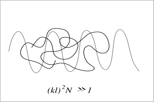
FIG. 2.: The test chain experiences the short wavelength melt density fluctuations and as a result it is weakly ”pinned”.

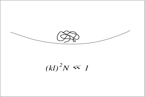
FIG. 3.: The interplay of the test chain and very long wavelength density fluctuations does not influence the Rouseian dynamics.

REFERENCES

- [1] H.Kinzelbach and H.Horner, J.Phys.I (France) 3, 1329 (1993)
- [2] T.A.Vilgis, J.Phys.I (France) 1, 1389 (1991)
- [3] W.Hess, Macromolecules 21, 2620 (1988)
- [4] K.S.Schweizer, J.Chem.Phys. 91, 5802 (1989)
- [5] K.S.Schweizer, J.Chem.Phys. 91, 5822 (1989)
- [6] K.S.Schweizer, Physica Scripta T 49, 99 (1993)
- [7] M.Fuchs and K.S.Schweizer, J.Chem.Phys. 106, 347 (1997)
- [8] M.Rehkopf, V.G.Rostishvili and T.A.Vilgis, J.Phys.II (France) 7, 1469 (1997)
- [9] D.Cule and Y.Shapir, Phys.Rev.E 53, 1553 (1996)
- [10] M.Mezard and G.Parisi, J.Phys.I (France) 1, 809 (1991)
- [11] S.E.Korshunov, Phys.Rev.B 48, 3969 (1993)
- [12] T.Giamarchi and P.LeDoussal, Phys.Rev.B 52, 1242 (1995)
- [13] H.Orland and Y.Shapir, Europhys.Lett. 30, 203 (1995)
- [14] T.Garel, G.Iori and H.Orland, Phys.Rev.B 53, R 2941 (1991)
- [15] T.Garel and H.Orland, Phys.Rev.B 55 ,226 (1997)
- [16] M.Doi and S.F.Edwards, The Theory of Polymer Dynamics, Clarendon Press, Oxford (1986)
- [17] P.G.deGennes, Scaling Concepts in Polymer Physics, Cornell Univ. Press, Ithaca, N.Y., 1979
- [18] D.Richter, L.Willmer, A.Zirkel, B.Fargo, L.J.Fetters and J.S.Huang, Macromolecules 27, 7437 (1994); D.S.Pearson, L.J.Fetters, W.W.Graessly, G.VerStrate and E.von Meerwal, Macromolecules 27, 711 (1994)
- [19] K.Kremer and G.S.Grest, J.Chem.Phys. 92, 5057 (1990)
- [20] B.Dünweg, G.S.Grest and K.Kremer, in Numerical Methods for Polymer Science (S.G.Whittington, ed.) IMA Volume in Mathematics and its Apllications 102, Springer-Verlag, 1998, p.159
- [21] V.G.Rostiashvili, M.Rehkopf and T.A.Vilgis, submitted to EPJB
- [22] M.E.Cates, J.Phys. (France) 46, 1059 (1985)
- [23] T.A.Vilgis, Phys.Rev.A 36, 1506 (1987); Physica A 153, 341 (1988); J.Phys.II (France) 2, 1961 (1992); P.Haronska and T.A.Vilgis, J.Chem.Phys. 102, 6586 (1995)
- [24] W.Paul, K.Binder, D.W.Heermann and K.Kremer, J.Chem.Phys. 95, 7726 (1991)
- [25] S.W.Smith, C.K.Hall and B.D.Freeman, J.Chem.Phys. 104, 5616 (1996)
- [26] A.Kopf, B.Dünweg and W.Paul, J.Chem.Phys. 107, 6945 (1997)
- [27] W.Paul, G.D.Smith and D.Y.Yoon, Macromolecules 30, 7772 (1997)
- [28] W.Paul, G.D.Smith, D.Y.Yoon, B.Farago, S.Rathgeber, A.Zirkel, G.Willner and D.Richter, Phys.Rev.Lett. 80, 2346 (1998)
- [29] J.S.Shaffer, J.Chem.Phys. 101, 4205 (1994)
- [30] J.S.Shaffer, J.Chem.Phys. 103, 761 (1995)
- [31] K.Okun, M.Wolfgardt, J.Bashnagel and K.Binder, Macromolecules 30, 3075 (1997)
- [32] G.Fredrickson and E.Helfand, J.Chem.Phys. 93, 2048 (1990)
- [33] V.G.Rostiashvili, Sov.Phys. JETP 70, 563 (1990)
- [34] V.G.Rostiashvili, M.Rehkopf and T.A.Vilgis, submitted to J.Phys. (France)
- [35] I.Ya.Erukhimovich and A.N.Semenov, Sov.Phys. JETP 63, 149 (1986)
- [36] G.Doetsch, Einführung in die Theorie und Anwendung der Laplace-Transformation, Birkhäuser Verlag, (Basel-Stuttgart, 1976)
- [37] J.Zinn-Justin, Quantum field theory and critical phenomena, Clarendon press, Oxford 1989
- [38] D.Forster, Hydrodynamic Fluctuations, Broken Symmetry and Correlation Functions, Benjamin Inc., Reading (1992)
- [39] W.Götze, in Liquids, freezing and glass transition, ed. by J.P.Hansen, D.Levesque and J.Zinn-Justin, Amsterdam, North-Holland, 1991