Theory of the Spin Reorientation Transition of Ultra-Thin Ferromagnetic Films

Abstract

The reorientation transition of the magnetization of ferromagnetic films is studied on a microscopic basis within Heisenberg spin models. Analytic expressions for the temperature dependent anisotropy are derived from which it is seen that the reduced magnetization in the film surface at finite temperatures plays a crucial role for this transition. Detailed phase diagrams in the temperature-thickness plane are calculated.

The direction of the magnetization of thin ferromagnetic films depends on various anisotropic energy contributions like surface anisotropy fields, dipole interaction, and eventually anisotropy fields in the inner layers. These competing effects may lead to a film thickness and temperature driven spin reorientation transition (SRT) from an out-of-plane ordered state at low temperatures to an in-plane ordered state at higher temperatures at appropriate chosen film thicknesses. Experimentally, this transition has been studied in detail for various ultra-thin magnetic films [1, 2, 3]. Recently, it was found by Farle et al. [4] that ultra-thin Ni-films grown on Cu(001) show an opposite behavior: the magnetization is oriented in-plane for low temperatures and perpendicular at high temperatures.

It has been shown by various authors that the mechanism responsible for the temperature driven transition can be understood within the framework of statistical spin models. While Moschel et al. [5] showed that the temperature dependence of the SRT is well described qualitatively within a quantum mechanical mean field approach, most other authors focused on classical spin models. Results obtained by extended Monte Carlo simulations [6, 7] as well as mean field calculations of classical Heisenberg models [8, 9, 10], although different in detail, agree in the sense that a temperature driven SRT is obtained. Very recently, the perturbative approach [9, 10] has been extended to itinerant systems [11]. Note, however, that due to an unsufficient treatment of the spin-orbit induced anisotropy in this work no SRT is possible for mono- and bilayers in disagreement with the above mentioned theories and with experiments.

While the SRT from a out-of-plane state at low temperatures to an in-plane state at high temperature is found to be due to a competition of a positive surface anisotropy and the dipole interaction the interesting new result for ultra-thin Ni-films is argued [4] to have its origin in a stress-induced uniaxial anisotropy energy in the inner layers with its easy axis perpendicular to the film. This anisotropy is in competition with the dipole interaction and a negative surface anisotropy. Theory confirms this picture [9, 10].

In this paper a systematic investigation of the parameter and thickness dependence of the reorientation transition and in particular a calculation of the corresponding phase diagrams is presented. The calculations are done in the framework of a classical ferromagnetic Heisenberg model consisting of $L$ two-dimensional layers on a simple cubic (001) or face centered cubic (001) lattice. The Hamiltonian reads

$$\mathcal{H}=-\frac{J}{2}\sum_{\langle ij\rangle}\mathbf{s}_{i}\cdot\mathbf{s}_{j}-\sum_{i}D_{\lambda_{i}}(s_{i}^{z})^{2}+\frac{\omega}{2}\sum_{ij}r_{ij}^{-3}\mathbf{s}_{i}\cdot\mathbf{s}_{j}-3r_{ij}^{-5}(\mathbf{s}_{i}\cdot\mathbf{r}_{ij})(\mathbf{r}_{ij}\cdot\mathbf{s}_{j}),$$ (1)

where $\mathbf{s}_{i}=(s_{i}^{x},s_{i}^{y},s_{i}^{z})$ are spin vectors of unit length at position $\mathbf{r}_{i}=(r_{i}^{x},r_{i}^{y},r_{i}^{z})$ in layer $\lambda_{i}$ and $\mathbf{r}_{ij}=\mathbf{r}_{i}-\mathbf{r}_{j}$. $J$ is the nearest-neighbor exchange coupling constant, $D_{\lambda}$ is the uniaxial anisotropy which depends on the layer index $\lambda=1\ldots L$, and $\omega=\mu_{0}\mu^{2}/4\pi a^{3}$ is the strength of the long range dipole interaction on a lattice with nearest-neighbor distance $a$ ($\mu_{0}$ is the magnetic permeability and $\mu$ is the effective magnetic moment of one spin). Note that only second order uniaxial anisotropies $D_{\lambda}$ enter the Hamiltonian (1). In our calculations we will restrict ourself to the case that all anisotropies are equal to $D_{v}$ except at one surface, where the value is $D_{s}$, as this scenario is sufficient for explaining the basic physics of the temperature driven reorientation transition.

The Hamiltonian (1) is handled in a molecular-field approximation, the reader is referred to [10] for further details. In the following we assume translational invariance within the layers and furthermore that the magnetization is homogeneous inside the film and only deviates at the surfaces, which is justified by numerical simulations [10]. Therefore we can set $\langle\mathbf{s}_{i}\rangle=\langle\mathbf{s}_{\lambda}\rangle$ if $\mathbf{s}_{i}$ is a spin in a volume layer ($\lambda=v$) or in a surface layer ($\lambda=s$). Now we must distinguish two cases:

• For $L<=2$ we get a system with only one (surface) layer with the effective interactions $\tilde{x}_{ss}=x_{0}+2x_{1}(1-L_{s}^{-1})$, where $x$ is either the coordination number, $z$, or the dipole sum, $\Phi$, respectively. In this case we have $L_{s}=L$ and $L_{v}=0$. The effective uniaxial anisotropy is $\tilde{D}_{s}=D_{s}+(L_{s}-1)D_{v}$ and the Curie temperature of the unperturbated system is $T_{c}(L)/J=\tilde{z}_{ss}/3$.

• For $L>2$ we get a system with two layers with the effective interactions $\tilde{x}_{ss}=x_{0}$, $\tilde{x}_{vs}=x_{1}$, $\tilde{x}_{vv}=x_{0}+2x_{1}(1-L_{v}^{-1})$, and $\tilde{x}_{sv}=2x_{1}L_{v}^{-1}$. Here we have $L_{s}=2$ and $L_{v}=L-2$. Note that the coupling between the volume spin and the surface spin is asymmetric. The effective uniaxial anisotropies are $\tilde{D}_{s}=D_{s}+D_{v}$ and $\tilde{D}_{v}=L_{v}D_{v}$, respectively. The critical temperature of the unperturbated system is given by

  $$\frac{T_{c}(L)}{J}=\frac{z_{0}}{3}+\frac{z_{1}}{3}\left(1-L_{v}^{-1}+\sqrt{1+L_{v}^{-2}}\right).$$

In this approach we are not restricted to films with integer values of the thickness. The number of next neighbors $z_{\delta}$ and the constants $\Phi_{\delta}$ containing the effective dipole interaction between the layers for different lattice types and orientations are listed in table 1.

lattice	$z_{0}$	$z_{1}$	$z_{\delta>1}$	$\Phi_{0}$	$\Phi_{1}$		$\Phi_{\delta>1}$
sc(001)	4	1	0	9.034	-0.	327	$\mathcal{O}(e^{-2\pi(\delta-1)})$
fcc(001)	4	4	0	9.034	1.	429	$\mathcal{O}(e^{-\sqrt{2}\pi(\delta-1)})$

Table 1: Numerical constants $z_{\delta}$ and $\Phi_{\delta}$ for sc(001) and fcc(001) lattices.

A perturbation theory to the mean field Hamiltonian can be applied considering the terms proportional to $\omega$ and $D_{\lambda}$ as small perturbations which is justified in view of the smallness of these parameters [9, 10]. In this framework we derived an analytical expression for the total anisotropy $K(T)$ of the system which is defined as the difference of the free energies of the in-plane state and the out-of-plane state. $K(T)$ depends on temperature only through the absolute value of the subsystem magnetizations $m_{\lambda}(T)$ calculated with the unperturbed Hamiltonian and is given by

$$K(T)=\sum_{\lambda}\tilde{D}_{\lambda}\left(1-3T\frac{m_{\lambda}(T)}{h_{\lambda}(T)}\right)-\frac{3\omega}{4}\sum_{\lambda,\lambda^{\prime}}m_{\lambda}(T)\tilde{\Phi}_{\lambda\lambda^{\prime}}L_{\lambda^{\prime}}m_{\lambda^{\prime}}(T).$$ (2)

$\mathbf{h}_{\lambda}=J\sum_{\lambda^{\prime}}\tilde{z}_{\lambda\lambda^{\prime}}\mathbf{m}_{\lambda^{\prime}}$ is the mean field in subsystem $\lambda$. If we neglect the narrow canted phase, the reorientation temperature $T_{r}$ is given by the condition $K(T_{r})=0$.

For the homogeneous case ($L<=2$) the magnetization is approximately given by

$$m^{2}(T)\approx\frac{1-T/T_{c}}{1-2T/5T_{c}}.$$

This approximation deviates less than 1% from the values obtained numerically. From (2) we then get

$$K(T)\approx\left(1-\frac{T}{T_{c}}\right)\left[\tilde{D}_{s}-\frac{3\omega L\tilde{\Phi}_{ss}}{4(1-2T/5T_{c})}\right],$$

from which the reorientation temperature is determined as

$$\frac{T_{r}}{T_{c}}\approx\frac{5}{2}-\frac{15\omega}{8}\frac{\Phi_{0}L+2\Phi_{1}(L-1)}{D_{s}+(L-1)D_{v}}$$

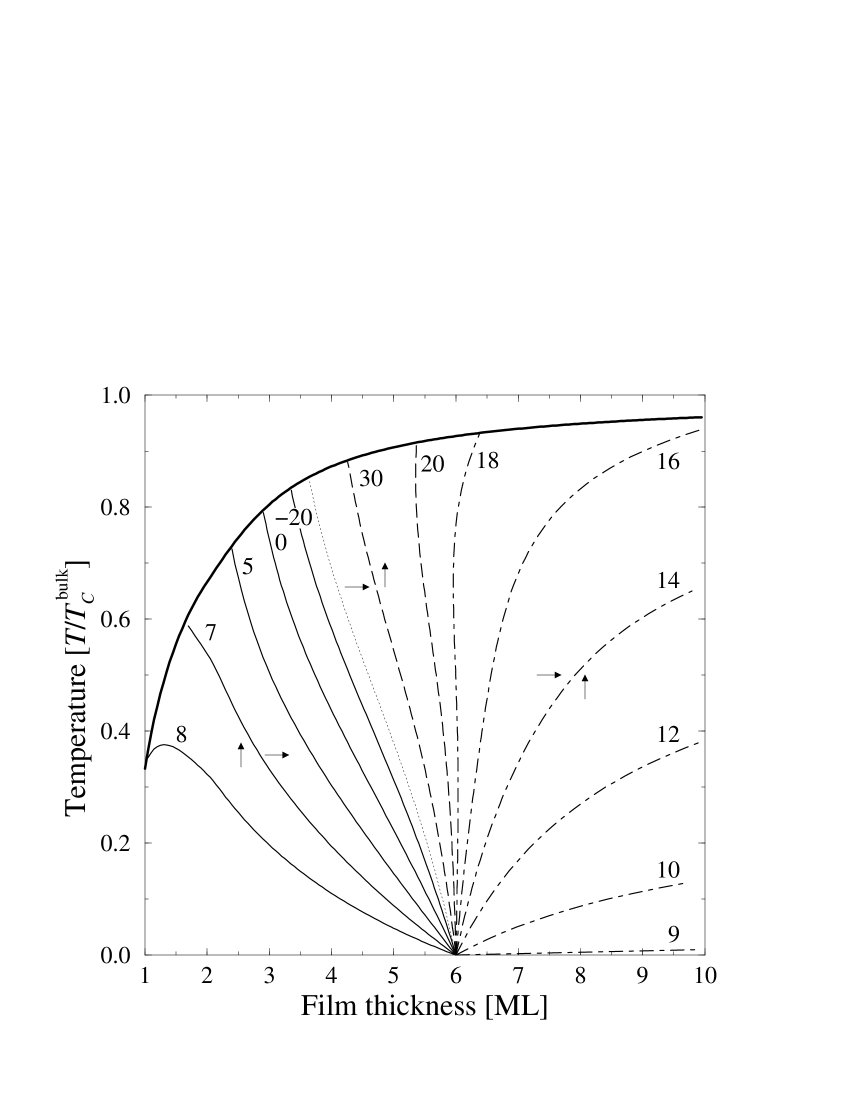
Figure 1: Phase diagrams of the fcc system for several values of $D_{v}/\omega$ (Numbers). $D_{s}/\omega$ is chosen so that in the ground state the SRT occurs at $L_{r}(T=0)=6$, i.e. $D_{s}=51.37\omega-5D_{v}$. The thick solid line represents the Curie temperature $T_{c}$ of the film, the solid lines are normal (Fe-type) SRTs, while the dashed lines are reversed (Ni-type) SRTs. The dash-dotted lines represent a third form of SRT, where the reorientation temperature $T_{r}$ grows with film thickness and does not necessarily reach $T_{c}$ for finite values of $L$. At the thin dotted line $D_{v}/\omega\rightarrow\pm\infty$, i.e. here the SRT occurs for $\omega=0$.

The phase diagram of the fcc(001) system calculated within this approach is shown in figure 1. One can distinguish three different reorientation schemes:

• For uniaxial volume anisotropies

  $$\frac{D_{v}}{\omega}<\frac{3}{4}(\Phi_{0}+2\Phi_{1})\approx 8.92\quad(\mathrm{fcc})$$

  we find a normal SRT from perpendicular to in-plane magnetization with increasing temperature and film thickness (solid lines in figure 1).

• If $D_{v}$ is large, we find a reversed SRT from in-plane to perpendicular magnetization with increasing temperature and film thickness (dashed lines in figure 1).

• In the intermediate range we obtain a third type of SRT where the magnetization switches from perpendicular to in-plane direction with increasing temperature, but with decreasing film thickness. (dash-dotted lines in figure 1).

This work was supported by the Deutsche Forschungsgemeinschaft through Sonderforschungsbereich 166. One of us (A.H.) would like to thank M. Farle for fruitful discussions.

References

- [1] R. Allenspach, J. Magn. Magn. Mater. 129, (1994) 160, and references therein.
- [2] D. P. Pappas, K.-P. Kämper, and H. Hopster, Phys. Rev. Lett. 64, (1990) 3179.
- [3] Z. Q. Qiu, J. Pearson, and S. D. Bader, Phys. Rev. Lett. 70, (1993) 1006.
- [4] M. Farle, B. Mirwald-Schulz, A. Anisimov, W. Platow, and K. Baberschke, Phys. Rev. B 55, (1997) 3708.
- [5] A. Moschel and K. D. Usadel, Phys. Rev. B 49, (1994) 12868.
- [6] S. T. Chui, Phys. Rev. B 50, (1994) 12559.
- [7] A. Hucht, A. Moschel, and K. D. Usadel, J. Magn. Magn. Mater. 148, (1995) 32.
- [8] A. Hucht and K. D. Usadel, J. Magn. Magn. Mater. 156, (1996) 423.
- [9] P. J. Jensen and K. H. Bennemann, Solid State Commun. 100 (1996) 585.
- [10] A. Hucht and K. D. Usadel, Phys. Rev. B 55 (1997) 12309.
- [11] T. Herrmann, M. Potthoff, and W. Nolting, Phys. Rev. B 58 (1998) 831.