Spectral Properties of Three Dimensional Layered Quantum Hall Systems

Although the quantized Hall effect is usually attributed to two-dimensional (2D) systems${}^{\hbox{\immediate{\bf{?}})}}$ the possibility of an occurrence in three-dimensional (3D) systems has been theoretically investigated early on .${}^{\hbox{\immediate{\bf{?}},\penalty 1000\hskip 0.91003pt plus 0.70004pt minus 0.70004pt{\bf{?}})}}$ In addition to some precursory experimental findings in 3D systems${}^{\hbox{\immediate{\bf{?}},\penalty 1000\hskip 0.91003pt plus 0.70004pt minus 0.70004pt{\bf{?}})}}$ there have been two classes of quasi-3D systems that show the integer quantum Hall effect: molecular crystals${}^{\hbox{\immediate{\bf{?}})}}$ and multi-layer quantum wells formed by graded GaAS/AlGaAs heterostructures.${}^{\hbox{\immediate{\bf{?}},\penalty 1000\hskip 0.91003pt plus 0.70004pt minus 0.70004pt{\bf{?}})}}$ Recently, the latter have attracted significant theoretical interest. The existence of a metallic phase for a finite range of energies and a new chiral 2D metallic phase on the surface have been proposed.${}^{\hbox{\immediate{\bf{?}},\penalty 1000\hskip 0.91003pt plus 0.70004pt minus 0.70004pt{\bf{?}},\penalty 1000\hskip 0.91003pt plus 0.70004pt minus 0.70004pt{\bf{?}})}}$ In ref. ? these 3D systems of 2D quantum Hall layers coupled by weak interlayer tunneling have been investigated using a network model. The existence of three phases: insulator, metal and quantized Hall conductor accompanied by extended surface states was shown by performing numerical transfer matrix calculations within the network model.

We will use the same kind of network model to investigate spectral properties of the 3D layered system. In doing so we will apply the methods used for the 2D Chalker-Coodington network model${}^{\hbox{\immediate{\bf{?}},\penalty 1000\hskip 0.91003pt plus 0.70004pt minus 0.70004pt{\bf{?}})}}$ which use the spectrum of the unitary network operator $U$ to determine the statistics of the eigenvalue spectrum of the underlying system.${}^{\hbox{\immediate{\bf{?}},\penalty 1000\hskip 0.91003pt plus 0.70004pt minus 0.70004pt{\bf{?}})}}$ This method has the advantage that after determining the critical energy $E_{\rm c}$ one can use the entire spectrum of eigenphases of $U(E_{\rm c})$ to investigate the critical spectral statistics.

The paper is structured in the following way: After an introduction to the network model we will use finite size scaling of the function $J_{0}(L,E)=\frac{1}{2}\langle s^{2}\rangle$, where $s$ is the level spacing in units of the average level spacing $\Delta$, to determine the critical point. At the critical point we are going to investigate the level spacing distribution function $P(s)$ and the number variance $\Sigma_{2}(N)=\langle(n-\langle n\rangle)^{2}\rangle$ of an energy interval containing on average $N=\langle n\rangle$ levels. We will see that, as in the 2D case, the following equation proposed in ref. ? holds:

$$\chi=\frac{\eta}{2d},$$ (1)

where $\chi=\lim_{N\rightarrow\infty}\lim_{L\rightarrow\infty}d\Sigma_{2}(N)/dN$ is the spectral compressibility, $d$ the spatial dimension of the system and $\eta$ the diffusion exponent, which is related to the fractal correlation dimension $D_{2}=d-\eta$.${}^{\hbox{\immediate{\bf{?}})}}$ We are also going to show that the tail region of the level spacing distribution shows an exponential decay at criticality, i.e. $P(s)\propto\exp(-\kappa s)$ and that as proposed in ref. ?:

$$\kappa=\frac{1}{2\chi}$$ (2)

The network model for the 3D layered system developed by Chalker and Dohmen (CD) is the natural generalization of the 2D Chalker-Coddington (CC) network model.${}^{\hbox{\immediate{?},\penalty 1000\hskip 0.91003pt plus 0.70004pt minus 0.70004pt{?})}}$ It is a model for electrons in 3D moving in a smooth disorder potential in 2D layers with a strong perpendicular magnetic field. In the classical limit, reached when the correlation length $l_{V}$ of the disorder potential $V$ is much larger than the magnetic length $l_{\rm c}$, the motion of the electrons can be decoupled into three independent components. The first with the smallest time scale is the cyclotron motion about a guiding center. Secondly, we have oscillations parallel to the magnetic field on an intermediate time scale and for long times we have a drift motion along the equipotential contours of $V$ in the plane perpendicular to the magnetic field.

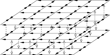
Fig.  1: The 3D Chalker-Dohmen network. It consists of layers of the 2D Chalker-Coddington model coupled by interlayer scattering matrices. The dashed double arrows mark the interlayer coupling nodes.

The network model simulates the system in the following way (see also Figure 1): The unidirectional channels in the 2D planes represent the equipotential contours of the potential in the plane. The random length of the contour is simulated by a random phase added to the electron at each channel link. The electrons travel along those lines until they reach a node of the network which represents a saddle point of the potential. At the saddle point they are scattered. The scattering amplitude $T=(1+\exp((E-u)/E_{\rm t})$ is determined by the electrons energy $E$ and the saddle point energy $u$, where $E_{\rm t}$ is the characteristic tunneling energy of the potential.${}^{\hbox{\immediate{?},\penalty 1000\hskip 0.91003pt plus 0.70004pt minus 0.70004pt{\bf{?}})}}$ In the following all the saddle point energies will be set to zero to avoid classical percolation effects.${}^{\hbox{\immediate{?},\penalty 1000\hskip 0.91003pt plus 0.70004pt minus 0.70004pt{\bf{?}},\penalty 1000\hskip 0.91003pt plus 0.70004pt minus 0.70004pt{\bf{?}})}}$ In addition to the scattering at the nodes at each link a scattering in the direction perpendicular to the plane takes place. This is accomplished by a scattering matrix of the form

$$S_{z}=\left(\begin{array}[]{cc}\cos\phi&\sin\phi\\ -\sin\phi&\cos\phi\end{array}\right),$$ (3)

giving us a transmission rate of $t=\sin\phi$, where $\phi$ is the same for all interlayer scatterings.

A state or wave function of the network is defined by a normalized vector $\Psi=(\psi_{1},\dots,\psi_{n})$ whose elements $\psi_{i}$ denote the complex amplitudes on the $n=2L^{3}$ network channels, where $L$ is the system size. Its time evolution is determined by the scattering matrices at the saddle points and the interlayer couplings which can be expressed by one unitary matrix $U$ the so called network operator:

$$\Psi(\tau+1)=U\Psi(\tau).$$ (4)

Actually, $U$ can be written as the product of a matrix $U_{2d}$ built from the independent network operators of the respective layer systems and an interlayer scattering matrix $S$ which takes care of the coupling of those systems, i.e. $U=U_{2d}S$. Both matrices are sparse with only 2 non-zero elements per column, which means that $U$ is also sparse with 4 non-zero elements per column. U is energy dependent through the energy dependence of the scattering matrices in the layers.

An energy eigenstate $\Psi_{E}$ of the underlying electronic system is a solution of the stationarity equation:

$$U(E)\Psi_{E}=\Psi_{E}$$ (5)

which corresponds to an eigenstate of $U(E)$ with eigenvalue unity. Such an eigenstate will occur only at discrete values of $E=E_{\rm c}$ which form the energy spectrum of the modeled system. However, it has been shown that the eigenphases $\omega_{\alpha}(E)$ of the unitary network operator $U(E)$ determined by the equation

$$U(E)\Psi_{\alpha}=e^{i\omega_{\alpha}(E)}\Psi_{\alpha}$$ (6)

show the same statistics as eigenenergies $E_{n}$ close to $E$.${}^{\hbox{\immediate{\bf{?}})}}$ Since the arguments in ref. ?, given for the Chalker-Coddington model, hold for any network model that includes an energy parameter we can use the so called quasienergies $\omega_{\alpha}(E)$, which can be considered an excitation spectrum at energy $E$, to determine the spectral properties of the 3D system.

Since the 3D network model exhibits three different phases, i.e. two phase transitions, our first task is to determine the critical points of those transitions. It has already been established in ref. ? that at energy $E_{\rm c_{1}}(t)(<0)$ the network exhibits an insulator-metal (IM) transition and symmetrical to the $E=0$ axis at energy $E_{\rm c_{2}}(t)=-E_{\rm c_{1}}(t)$ a metal-quantum Hall conductor (MQH) transition for every $t$. The states in the quantum Hall conductor are all localized as in the insulator phase except for the fact that for hard wall boundary conditions there exist extended surface states separated from the localized bulk states. In our investigation we are using mostly periodic boundary conditions, but we will comment on the hard walled systems if results differ significantly.

The width $W=E_{\rm c_{2}}-E_{\rm c_{1}}$ of the metallic phase was shown to depend on the coupling $t$ in the following way: $W(t)\propto t^{1/\nu_{2d}}$, where $\nu_{2d}\approx 2.3$ is the critical exponent of the localization length in 2D quantum Hall Systems.${}^{\hbox{\immediate{?})}}$ This knowledge was used to narrow the range for our search of the critical energies.

Fig.  2: The scaling variable $J_{0}$ as a function of $E$ for different system sizes and $t=0.2$. At $E\approx 2.2$ all the curves meet in a single point. The inset shows the one-parameter dependence of $J_{0}$ on $L/\xi(E)$.

The critical energies are determined by finite size scaling. As a scaling variable the quantity $J_{0}=\frac{1}{2}\langle s^{2}\rangle$ is used. This function reflects the transition of the spectral correlations from Gaussian unitary ensemble (GUE) to Poisson statistics when we cross from the metallic phase into a localized regime. The values $J_{0}=0.590$ in the metallic and $J_{0}=1$ in the localized regime are well known from random matrix theory (RMT).${}^{\hbox{\immediate{\bf{?}})}}$

Fig.  3: The scaling variable $J_{0}$ as a function of $E$ for different system sizes and $t=0.2$. At $E\approx-2.2$ all the curves meet in a single point. The inset shows the one-parameter dependence of $J_{0}$ on $L/\xi(E)$.

In Figs. 2 and 3 we can see the function $J_{0}(E)$ at $t=0.2$ for different system sizes $L$ and energies $E>0$ and $E<0$, respectively. The curves for different $L$ in both figures intersect in single points at $E_{c_{1}}\approx-2.2$ and $E_{c_{2}}\approx 2.2$ with $J_{0}^{\rm c}\approx 0.68$ in both cases. These points mark the IM and MQH transitions. Assuming the validity of one-parameter scaling, i.e. $J_{0}(E,L)=f(L/\xi(E))$, and the existence of the localization length $\xi(E)$ that shows the power law behavior $\xi(E)\propto|E-E_{\rm c}|^{-\nu}$, one can re-scale $L$ so that the data of $J_{0}$ as a function of $L/\xi$ for consecutive energies $E$ overlap with each other. Within statistical accuracy all points fall onto one common curve independent of $L$ and $E$. This can be seen in the insets of the two figures where $J_{0}(E,L)$ is plotted against $L/\xi(E)$.

$t$	$E_{\rm c}$		$\nu$		$J_{0}^{\rm c}$
$0.1$	$-1.6$	$\pm 0.2$	$1.2$	$\pm 0.5$	$0.73$	$\pm 0.05$
$0.2$	$2.17$	$\pm 0.03$	$1.33$	$\pm 0.18$	$0.669$	$\pm 0.003$
$0.2$	$-2.04$	$\pm 0.02$	$1.27$	$\pm 0.08$	$0.682$	$\pm 0.002$
$0.4$	$3.08$	$\pm 0.03$	$1.5$	$\pm 0.2$	$0.68$	$\pm 0.01$
$0.5$	$3.33$	$\pm 0.03$	$1.45$	$\pm 0.1$	$0.69$	$\pm 0.01$

Table  I: The results for the 4-parameter fit of eq. (7).

In order to calculate the critical exponent $\nu$ we expand the finite-size scaling function around the critical point:

$$J_{0}(E,L)\approx J_{0}^{\rm c}+B(E-E_{\rm c})L^{1/\nu}.$$ (7)

We can now either determine $\nu$, $J_{0}^{\rm c}$, $E_{\rm c}$ and $B$ by a four-parameter fit or we can take the energy derivative of eq. (7), which gives us $dJ_{0}(E,L)/dE\propto L^{1/\nu}$ and perform a two parameter linear fit to a double-log plot of the slope of $J(E)$ as a function of $L$ at the critical point $E_{\rm c}$. The results for the 4-parameter fit are shown in Table I for different values of the coupling $t$. The linear fit of the slope data yields essentially the same results as the 4-parameter fit (see Table II). The results for the exponent $\nu$ are in agreement with earlier numerical results for layered 3D systems${}^{\hbox{\immediate{\bf{?}},\penalty 1000\hskip 0.91003pt plus 0.70004pt minus 0.70004pt{?})}}$ ($\nu=1.35\pm 0.15$ and $\nu=1.45\pm 0.25$) and 3D Anderson models${}^{\hbox{\immediate{\bf{?}},\penalty 1000\hskip 0.91003pt plus 0.70004pt minus 0.70004pt{\bf{?}},\penalty 1000\hskip 0.91003pt plus 0.70004pt minus 0.70004pt{\bf{?}})}}$ ($\nu=1.43\pm 0.06$ and $\nu=1.34\pm 0.10$) with broken time reversal symmetry. The values for the critical energy also agree with the results of Chalker and Dohmen.${}^{\hbox{\immediate{?})}}$

$t$	$E_{\rm c}$		$\nu$
$0.1$	$-1.6$	$\pm 0.05$	$1.2$	$\pm 0.2$
$0.2$	$-2.2$	$\pm 0.05$	$1.34$	$\pm 0.06$
$0.2$	$2.2$	$\pm 0.1$	$1.32$	$\pm 0.04$
$0.4$	$3.1$	$\pm 0.1$	$1.6$	$\pm 0.4$
$0.5$	$3.4$	$\pm 0.1$	$1.3$	$\pm 0.1$

Table  II: The results for $\nu$ obtained from the derivatives $dJ_{0}/dE$ at $E_{\rm c}$.

Now that we know the critical energies $E_{\rm c}(t)$ we can concentrate on the investigation of the spectral properties at criticality. We start by looking at the critical level spacing distribution $P(s)$. We are going to compare it to the Poisson distribution ($P_{\rm P(s)}=\exp(-s)$) in the localized and the GUE distribution ($P_{\rm GUE}(s)=\frac{32}{\pi^{2}}s^{2}\exp\left(-\frac{4}{\pi}s^{2}\right)$) in the metallic regime known from RMT.${}^{\hbox{\immediate{?})}}$ The critical $P(s)$ shows characteristics of both of these distributions. In Fig. 4 we can see the critical $P(s)$ for $t=0.2$ and several system sizes. As expected they are independent of the system size and all fall on the same curve. They also obviously differ strongly from the Poisson and GUE distributions. Those distributions were obtained from networks with periodic boundary conditions. The inset of Fig. 4 shows a comparison of the periodic boundary case with a critical distribution of a system with hard wall boundaries (HWB) in one direction. We can see that in the HWB case $P(s)$ is shifted towards the Poisson distribution which means a different $J_{0}^{c}\approx 0.7$. This has also been observed in other 3D systems.${}^{\hbox{\immediate{\bf{?}})}}$ We also found a slightly increased value for $E_{c}$ which if confirmed has to be investigated in later publications (see also refs. ? and ?).

Fig.  4: The critical level spacing distribution $P(s)$ for $t=0.2$ and several system sizes compared to the Poisson and GUE distributions. The inset shows the critical $P(s)$ for two different boundary conditions.

A closer investigation of the shape of the critical distribution reveals that for small values of $s$ it resembles the GUE case. The inset in Fig. 5 shows the small $s$ behavior and we can see that $P(s)\propto s^{2}$ for all couplings $t$. This reflects the level repulsion due to the multifractal eigenstates which, like the homogeneously smeared out metallic eigenstates, cover the entire system. On the other hand, a look at the behavior for large values of $s$ shows an exponential decay of the tail of $P(s)$ (see Fig. 5) which is typical for the Poisson distribution and in contrast to the Gaussian tail of the GUE case.

Fig.  5: The tail of the critical $P(s)$ for $t=0.2,0.4,0.5$ compared to the GUE and Poisson case. The left inset shows the small $s$ behavior of $P(s)$ compared to the function $s^{2}$. The right inset is the level number variance at criticality.

Compared to the Poisson case, the critical distribution decays faster with $P(s)\propto\exp(-\kappa s)$ where $\kappa=1.76\pm 0.04$ for $t=0.2$, which is the coupling where we got the most statistics. According to ref. ?, which predicted this exponential decay, the factor $\kappa$ is connected to the spectral compressibility $\chi$ via eq. (2). This leads us to the next step in our investigation, the determination of $\chi$.

In the right inset of fig. 5 we can see the level number variance $\Sigma_{2}$ whose slope gives us $\chi$. The results for the different coupling strengths all agree with each other and we again took the value for $\chi$ from our data for $t=0.2$. We obtained: $\chi=0.286\pm 0.003$ which gives us according to eq. (2) $\kappa=1.75\pm 0.01$ which is in good agreement with the directly obtained value of $\kappa$. These values for $\chi$ and $\kappa$ are also quite close to the ones obtained in ref. ? for a 3D Anderson model with time reversal symmetry. Furthermore, we can connect the spectral compressibility directly to the multifractal critical wave functions. This was done in ref. ? resulting in eq. (1). If we use $\chi$ we obtain a value of $\eta=1.72\pm 0.02$ or $D_{2}=1.28\pm 0.02$. If we compare $D_{2}$ with direct results for the network model ($1.3\pm 0.1$${}^{\hbox{\immediate{\bf{?}})}}$) or 3D Anderson models without time reversal symmetry ($1.7\pm 0.2$,${}^{\hbox{\immediate{\bf{?}})}}$$\approx 1.5$${}^{\hbox{\immediate{\bf{?}})}}$) we see that eq. (1) holds within the errors. Although the result for $D_{2}$ taken from eq. 1, which fits very well to the direct result from ref. ?, is a little smaller than those of other investigations.

In conclusion, the numerical investigation of the spectral statistics of a network model for a three dimensional layered quantum Hall system for different coupling strengths between the layers showed that the phase transitions from metallic to localized regimes all have the same characteristics. The critical exponent $\nu\approx 1.3$ is in agreement with other results for similar systems. Furthermore, the relations (1) and (2) were verified to a high degree of accuracy within the network model. This is an improvement to other 3D models (all of them with time reversal symmetry) where the two equations could also be verified but with much larger errors.${}^{\hbox{\immediate{?})}}$ This shows that the usage of network models, apart from their advantages for the investigation of time evolution, gives us a more efficient way to investigate spectral properties.

The author would like to thank Y. Ono for valuable discussions and the Deutsche Forschungsgemeinschaft (DFG) for their financial support.

References

- [1]
- [2] M. Janssen, O. Viehweger, U. Fastenrath and J. Hajdu: Introduction to the Theory of the Integer Quantum Hall Effect (VCH, Weinheim, New York, Basel, Cambridge, Tokyo, 1994).
- [3] M. Y. Azbel: Solid State Comm. 54 (1985) 127.
- [4] M. Y. Azbel and O. Entin-Wohlman: Phys. Rev. B 32 (1985) 562.
- [5] R.G. Mani: Phys. Rev. B 41 (1989) 7922.
- [6] U. Zeitler , A. G. M. Jansen, P. Wyder and S. S. Murzin: J. Phys. Cond. Matt. 6 (1994) 4289.
- [7] S. Valfells, J.S. Brooks, Z. Wang, S. Takasaki, J. Yamada, H. Anzai and M. Tokumoto: Phys. Rev. B 54 (1996) 16413.
- [8] H.L. Störmer: Phys. Rev. Lett. 56 (1986) 85.
- [9] Y. J. Wang, B. D. Mccombe, R. Meisels, F. Kuchar and W. Schaff: Phys. Rev. Lett. 75 (1995) 906.
- [10] J. T. Chalker and A. Dohmen: Phys. Rev. Lett. 75 (1995) 4496.
- [11] Z. Wang: Phys. Rev. Lett. 79 (1997) 4002.
- [12] L. Balents and M. P. A. Fisher: Phys. Rev. Lett. 76 (1996) 2782.
- [13] J. T. Chalker and P. D. Coddington: J. Phys. C 21 (1988) 2665.
- [14] D. H. Lee, Z. Wang and S. Kivelson: Phys. Rev. Lett. 70 (1993) 4130.
- [15] R. Klesse and M. Metzler: Phys. Rev. Lett. 79 (1997) 721.
- [16] M. Metzler and I. Varga: J. Phys. Soc. Jpn. 67 (1998) 1856.
- [17] R. Klesse and M. Metzler: Europhys. Lett. 32 (1995) 229.
- [18] J. T. Chalker, V. E. Kravtsov and I. V. Lerner: JETP Lett. 64 (1996) 386.
- [19] M. Janssen: Ph.D. Thesis, Universität zu Köln 1990.
- [20] B. L. Altshuler, I. Kh. Zharekeshev, S. A. Kotochigova and B. Shklovskii: Sov. Phys.-JETP 67 (1988) 625.
- [21] H. A. Fertig: Phys. Rev. B 38 (1988) 996.
- [22] M. Metzler: Ph.D. Thesis, Universität zu Köln 1996.
- [23] M. Metzler: to be published.
- [24] M. L. Mehta: Random Matrices, 2nd ed. (Academic Press, New York, 1991).
- [25] T. Ohtsuki, B. Kramer and Y. Ono: J. Phys. Soc. Jpn. 62 (1993) 224.
- [26] K. Slevin and Tomi Ohtsuki: Phys. Rev. Lett. 78 (1997) 4083.
- [27] E. Hofstetter and M. Schreiber: Europhys. Lett. 21 (1993) 933.
- [28] E. Hofstetter and M. Schreiber: Phys. Rev. B 49 (1994) 14726.
- [29] D. Braun, G. Montambaux and M. Pascaud: Phys. Rev. Lett. 81 (1998) 1062.
- [30] B. Elattari and M. Metzler: to be published.
- [31] H. Potempa and L. Schweitzer: to appear in Physica A.
- [32] I. Kh. Zharekeshev and B. Kramer: Jpn. J. Appl. Phys. 34 (1995) 4361.
- [33] B. Huckestein and Rochus Klesse: to be published (cond-mat 9805038).
- [34] T. Ohtsuki and T. Kawarabayashi: J. Phys. Soc. Jpn 66 (1997) 314.
- [35] T. Terao: Phys. Rev. B 56 (1997) 975.