Average persistence in random walks

          Heiko Rieger$(*)$ and Ferenc Iglói$(**)$ $(*)$ HLRZ, Forschungszentrum Jülich, 52425 Jülich, Germany
Institut für Theoretische Physik, Universität zu Köln, 50923 Köln, Germany $(**)$ Research Institute for Solid State Physics and Optics, H-1525 Budapest, P.O.Box 49, Hungary
Institute for Theoretical Physics, Szeged University, H-6720 Szeged, Hungary PACS. 64.60.Ak, 75.10.Hk — Random walk models, persistence probability, anomalous diffusion in disordered environments, random quantum spin chains Abstract. — We study the first passage time properties of an integrated Brownian curve both in homogeneous and disordered environments. In a disordered medium we relate the scaling properties of this center of mass persistence of a random walker to the average persistence, the latter being the probability $\overline{P}_{\rm pr}(t)$ that the expectation value $\langle x(t)\rangle$ of the walker’s position after time $t$ has not returned to the initial value. The average persistence is then connected to the statistics of extreme events of homogeneous random walks which can be computed exactly for moderate system sizes. As a result we obtain a logarithmic dependence $\overline{P}_{\rm pr}(t)\sim\ln(t)^{-\overline{\theta}}$ with a new exponent $\overline{\theta}=0.191\pm 0.002$. We note on a complete correspondence between the average persistence of random walks and the magnetization autocorrelation function of the transverse-field Ising chain, in the homogeneous and disordered case.

First passage time or persistence problems have a long history in the physical literature [1]. Recently they gained a lot of interest, since the persistence exponents, describing the asymptotic behavior of first passage time probabilities, are shown to be independent dynamical critical exponents, which have been calculated for various models exactly[2, 3]. Not much is known about analogous quantities in systems with quenched disorder, for instance the random walk (or diffusion) in a disordered environment [4], which is in the one-dimensional case the Sinai-model[5]. For this model the first passage / persistence exponent for a single walker has been determined by us in a previous work [6]. In this letter we introduce and study the concept of average persistence of random walks both in homogeneous and random environments.

We consider a random walk with nearest neighbor hopping in one dimension defined by the Master equation

$$p_{i}(t=0)=\delta_{i,1}\;,\quad\frac{d}{dt}p_{i}(t)=-(w_{i,i-1}+w_{i,i+1})p_{i}(t)+w_{i-1,i}p_{i-1}(t)+w_{i+1,i}p_{i+1}(t)$$ (1)

describing the time evolution of the probability $p_{i}(t)$ for the walker to be at site $i$ after time $t$ when having been initially at site $i=1$. The homogeneous random walk is defined via uniform transition rates $w_{i,i+1}=w_{i+1,i}=1/2$ and the random walk in a disordered environment is modeled by choosing the transition rates to be quenched random variables that obey a particular distribution, e.g. the uniform distribution $\pi_{\rm uni}$ given by $w_{i,i\pm 1}=1$ for $0<w_{i,i\pm 1}<1$ and $0$ otherwise, or the binary distribution

$$\pi_{\rm bin}(w_{i,i-1})=\frac{1}{2}\delta(w_{i,i-1}-\lambda)+\frac{1}{2}\delta(w_{i,i-1}-\lambda^{-1})\;,\quad w_{i,i+1}=1\quad\forall i$$ (2)

with $\lambda$ some arbitrary parameter. For the disordered case physical observables have to be averaged over this distribution $\pi$ which is denoted by square brackets $[\ldots]_{\rm av}$. Note we consider the general case of asymmetric hopping rates $w_{i,i+1}\neq w_{i+1,i}$ and we do not confine ourselves to the so called random force model with correlated transition probabilities parameterized as $w_{i,i\pm 1}=A\exp(\pm\phi_{i})$ with random, uncorrelated potentials $\phi_{i}$ on each site.

In order to define single walker persistence probabilities we put an adsorbing boundary at site $i=0$, which means that we set $w_{1,0}=0$ and also introduce a finite size length scale $L$ into the system by putting another adsorbing boundary at $i=L+1$, i.e. setting $w_{L+1,L}=0$. Now we define the length scale dependent single walker persistence $P_{\rm pr}(L,t)$ to be the probability that a walker does not cross its starting point (i.e. does not get trapped at site $i=0$) within the time interval $t$. The following arguments[6] will then lead us to a scaling form for $P_{\rm pr}(L,t)$: a) the typical time the walker needs to reach the site $L+1$ scales like $t_{\rm typ}\sim L^{2}$ in the case with symmetric transition rates and like $\ln t_{\rm typ}\sim\sqrt{L}$ in the asymmetric case, the Sinai-model, b) the asymptotic limit $P_{\rm surv}(L)=\lim_{t\to\infty}P_{\rm pr}(t,L)=\lim_{t\to\infty}p_{L+1}(t)$, which is what we call a survival probability, behaves like $P_{\rm surv}(L)\sim L^{-1}$ in the symmetric case and like $P_{\rm surv}(L)\sim L^{-\theta_{a}}$ with $\theta=1/2$ in the Sinai-model. Hence we expect

$$[P_{\rm pr}(L,t)]_{\rm av}\sim\left\{\begin{array}[]{lcl}L^{-\theta_{s}}\cdot\tilde{p}_{s}(L^{2}/t)&&({\rm symmetric\;case})\\ L^{-\theta_{a}}\cdot\tilde{p}_{a}(\sqrt{L}/\ln t)&&({\rm asymmetric\;case})\end{array}\right.$$ (3)

where the persistence exponents are $\theta_{s}=1$ for the symmetric case and $\theta_{a}=1/2$ for the asymmetric case, and the scaling functions behave like $\tilde{p}_{s}(x)\to x^{\theta_{s}/2}$ and $\tilde{p}_{a}(x)\to x^{2\theta_{a}}$ for $x\to\infty$ and $\tilde{p}_{s/a}(x)\to const.$ for $x\to 0$. In the infinite system size limit one thus has for persistence probability $P_{\rm pr}(t)$ in the asymmetric case $P_{\rm pr}(t)=\lim_{L\to\infty}P_{\rm pr}(L,t)\propto\ln(t)^{-2{\theta}_{a}}$, a logarithmically slow decay reminiscent of the critical dynamics of the surface magnetization of the random transverse Ising chain[14] (RTIC). This is not incidental: the equivalence of the surface magnetization in the latter quantum spin chain and the survival probabilities of random walks has been formulated the first time in [7] and further analogies between anomalous diffusion and the RTIC have been uncovered recently [6, 8].

Figure 1: The average persistence $[\overline{P}_{\rm pr}(L,t)]_{\rm av}$ to the power $-1/2\overline{\theta}_{a}$ versus $\ln t$, which should yield a straight line in the limit $L\to\infty$, for different finite size scaling length $L$. The data are for uniform distribution and averaged over 50.000 samples. We used an estimate $\overline{\theta}_{a}=0.19$ to obtain an optimal data collapse in the scaling region. The straight line indicates the asymptotic result for the infinite system $L\to\infty$.

It is known that diffusion in the Sinai model is different from normal diffusion in many respects[4]. Consider for instance one particular disorder realization. Then an initially narrow probability distribution of a walker peaked around, say, $x(t=0)=0$ does not broaden with time, only its expectation value $\langle x(t)\rangle=\sum_{i}i\cdot p_{i}(t)$ diffuses logarithmically slowly away from its starting point. Therefore, in this situation in addition to the single walker persistence one should also consider the persistence properties of the average position of the walker $\langle x(t)\rangle$, the average persistence $\overline{P}_{\rm pr}(t)$: This is the probability that up to a specified time $t$ the average position of the walk in a particular environment has always been on one side of the starting point, i.e. $\forall 0<t^{\prime}<t:\;\langle x(t^{\prime})\rangle>0$.

To study the average persistence we consider again a finite size situation where we put an adsorbing boundary at $i=-L$ and one at $i=L$ (note that now a single walker is not adsorbed when crossing the starting point but only when he leaves the finite strip of width $2L$ centered around $i=0$). Then the average persistence $\overline{P}_{\rm pr}(L,t)$ obeys the same scaling form as in the second line of (3), but the single walker persistence exponent $\theta_{a}$ replaced by the average persistence exponent $\overline{\theta}_{a}$:

$$[\overline{P}_{\rm pr}(L,t)]_{\rm av}\sim L^{-\overline{\theta}_{a}}\cdot\overline{p}_{a}(\sqrt{L}/\ln t)\;.$$ (4)

Moreover, the persistence probability for the infinite system decays again logarithmically slow: $\overline{P}_{\rm pr}(t)\propto\ln(t)^{-2{\overline{\theta}}_{a}}$. Recently it has been conjectured for the random force model[8] that the exponent $\overline{\theta}_{a}$ is related to the golden mean via $\overline{\theta}_{a}=(3-\sqrt{5})/4\approx 0.191$. In fig. 1 we show numerical data that have been obtained by a numerical calculation of $P_{\rm pr}(L,t)$ via diagonalization of the linear operator on the r.h.s. of eq.(1), which indicate that this might also hold for the general asymmetric case.

In what follows we will demonstrate how to obtain a precise estimate of the average persistence exponent $\overline{\theta}_{a}$. Since in the limit $t\to\infty$ the average persistence probability is given by $\overline{P}_{\rm surv}\sim L^{-\overline{\theta}_{a}}$, the computation of the survival probability $\overline{P}_{\rm surv}$ will lead us to the desired result. We will now relate this survival probability to a problem in the statistics of extreme events of homogeneous random walks. To this end we consider the binary distribution $\pi$ in (2) in the limit $\lambda\to 0$, which means that one can discriminate between ”forward” bonds $(i,i+1)$, which are those for which $w_{i,i-1}=\lambda\to 0$, i.e. those where almost only (with probability $1/(1+\lambda)\to 1$ jumps from $i$ to $i+1$ occur, and ”backward” bonds, which have $w_{i,i-1}=\lambda^{-1}\to\infty$, implying almost always jumps from $i$ to $i-1$ (again with probability $\lambda^{-1}/(1+\lambda^{-1})\to 1$). This implies that when sketching the transition rates as configuration as is done in fig. 2 the disorder configuration can be done visualized as a random landscape with hills and valleys. Thus a walker starting at $i=0$ is on average first driven to the first minimum $M_{1}$, and considering the finite size situation where $L=L_{1}$ this disorder configuration counts as a surviving configuration, since the walker in average spends most of its time at $M_{1}$. Increasing the length scale $L$ further beyond $L_{2}$ will then drive the average position of the walker over the barrier $B$ into the valley $M_{3}$ at negative coordinates, which means that this configuration is dead, i.e not surviving.

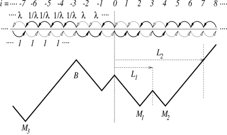
Figure 2: Sketch of the random landscape that corresponds to the binary distribution (2). In the limit $\lambda\to 0$ transitions corresponding to broken arrows will rarely occur whereas transitions corresponding to full arrows will occur with probability close to one. For further details describing the effective dynamics see text.

Thus we conclude that the computation of $\overline{P}_{\rm surv}$ amounts to counting all surviving configurations of a random landscape, i.e. a homogeneous random walk, in the manner described above and the ratio of surviving configurations is just $\overline{P}_{\rm surv}$. In other words we consider random walks of length $2L$, corresponding to realizations of the transition probabilities according to (2) in a strip of width $2L$ centered around the starting point, and say that it is in average surviving if certain conditions are fulfilled. These conditions are checked by inspecting the random landscape generated by the disorder configuration (i.e the transition rates): one scans the landscape in both directions from the starting point and denotes with $h(i)$ ($i=-L,-L+1,\ldots,-1,0,1,2,\ldots,L$) the position of the walker (or height of the landscape) at step (or site) $i$. We define the extreme events to the right and to the left of $i=0$ by $x_{\rm max/min}(i)={\rm max/min}\{h(j)|0\leq j\leq i\}$ and $y_{\rm max/min}(i)={\rm max/min}\{h(j)|-i\leq j\leq 0\}$, respectively, and check iteratively (from $i=1$ to $i=L$) whether

$$x_{\rm min}(i)>y_{\rm min}(i)\quad{\bf and}\quad x_{\rm max}(i)>y_{\rm max}(i)\;.$$ (5)

If this happens for some site $i$, as it does for $i=8$ in fig. 2, it means that there is a lower minimum on the left side of the starting point ($x_{\rm min}<y_{\rm min}$) and that the walker can go there since the barrier in between is low enough ($x_{\rm max}<y_{\rm max}$). This implies that this configuration is dead.

In the inset of fig. 3 we show the results for a numerical estimate of the survival probability $\overline{P}_{\rm surv}(L)$ by inspecting 10⁵ random walk configuration for different system sizes — the data fit well to a power law with the exponent $\overline{\theta}_{a}=0.19$. Next we implemented a recursive routine that computes the number of surviving configuration according to the above extreme events criterion (5) exactly. Here we took special care to the degenerate minima (like $M_{1}$ and $M_{2}$ in fig. 2), in which case we assumed the arithmetic mean of the location of the two to be the effective position ($L_{1}$ in fig. 2). From these exact data for system sizes up to $L=14$ we can extract via $\overline{\theta}_{a}(L_{a},L_{b})=-\ln(P_{\rm surv}(L_{a})/P_{\rm surv}(L_{b}))/\ln(L_{a}/L_{b})$ an effective finite size exponent that approaches the exact value. In fig. 3 we show these exact data for $L_{a}=L=L_{b}+1$ and $L_{a}=L=L_{b}+2$. Finally, from a standard series extrapolation procedure[9] applied to these data we obtain our best estimate which is

$$\overline{\theta}_{a}=0.191\pm 0.002\;,$$ (6)

in very good agreement with the conjectured value $\overline{\theta}_{a}=(3-\sqrt{5})/4=0.19098\ldots$ for the random force model[8].

Figure 3: The effective finite size exponent $\overline{\theta}_{a}$ from exact values for $\overline{P}_{\rm pr}(L)$ via complete enumeration of all surviving configuration. The asymptotic value $\overline{\theta}_{a}=0.191$ obtained by series extrapolation methods is also shown. The insert shows the result for $\overline{P}_{\rm pr}(L)$ via stochastic enumeration for larger system sizes, giving $\overline{\theta}_{a}=0.19\pm 0.01$.

Although the concept of an average persistence seems to be based upon the special feature of non-dispersive diffusion in the Sinai model, which we described above, it turns out that there is an analogy to it in normal diffusion, too. To show this, we first introduce the integrated position of the walker at step $t$ as $I_{t}=\sum_{\tau=1}^{t}i_{\tau}$, where $i_{\tau}$ is its position at time-step $\tau$. Then, we define the center of mass persistence through the survival condition for the integrated position as $I_{t^{\prime}}\geq 0$ for $0<t^{\prime}<t$. For the disordered case we define a center of mass position via

$$C(i)=\sum_{j=-i}^{i}j\cdot M(h(j))\;.$$ (7)

where the weights $M(h(j))$, which are proportional to the average time the walker spent at a given site, depend on the random configurations. In a strip $(-L\leq i\leq L)$ with adsorbing boundaries the survival condition of the average position in the large $t$-limit is $C(i)\geq 0$ for $i=1,\ldots,L$, which is equivalent to the survival condition in (5). For the extreme binary distribution, we consider here, the weight function is singular, such that $M(h^{\prime})/M(h)\to 0$ for $h^{\prime}<h$, which is a consequence of the limit $\lambda\to 0$ for the distribution (2). Since the form of the distribution of the random transition rates is generally irrelevant one expects that the scaling properties of the average persistence and those of the center of mass persistence in (7) are equivalent for other type of distributions as well.

For a homogeneous walk one can also study the center of mass persistence or the survival probability of the $I_{t}$ integrated position. This type of problem has already been considered by Sinai[10] for a discrete model and later by Burkhardt[11] for the continuum model. According to these exact results in a homogeneous infinite system the long-time behavior of the average persistence is given by $\lim_{L\to\infty}\overline{P}_{pr}^{hom}(L,t)\sim t^{-1/4}$. We use this result to write for finite systems the scaling conjecture:

$$\overline{P}_{pr}^{hom}(L,t)=L^{-\overline{\theta}_{hom}}\overline{p}_{hom}(L/t)\;$$ (8)

with $\overline{\theta}_{hom}=1/4$ and the scaling function behaves like $\overline{p}_{hom}(x)\sim x^{\overline{\theta}_{hom}}$ for $x\to\infty$ and $\overline{p}_{hom}(x)\to const$ for $x\to 0$. The scaling combination, $x=L/t$ in (8), follows from the scaling properties of the Brownian motion. In $t$ steps the walker typically crosses its starting position $\sim t^{1/2}$ times and its displacement is typically of $\sim t^{1/2}$, thus the integrated displacement is $\sim t$, from which the scaling relation $L\sim t$ follows. It is interesting to note that the integrated Brownian curve is an isotropic critical object, with a correlation length critical exponent $\nu=1$, as for the two-dimensional Ising model.

By an exact enumeration up to $L=30$ we have checked the relation in (8) in the limit $t\to\infty$ and got an estimate $\overline{p}_{hom}(x=0)=0.6183(3)$ for the scaling function. It is amusing to note that the above value agrees, within the accuracy of the estimate, with the inverse of the golden mean ratio $1/\tau=2/(\sqrt{5}+1)=0.6180$.

Concluding, we introduced the concept of average persistence in random walks and studied its scaling properties in homogeneous and in disordered environments. The finite-size scaling behavior of $\overline{P}_{pr}(L,t)$ as given in (4) and (8) involve new exponents: $\overline{\theta}$ in (6) and $\overline{\theta}_{hom}=1/4$ for the disordered and homogeneous problems, respectively. It is interesting to note on an analogy between the finite-size scaling form of the average persistence of random walks and that of the magnetization autocorrelation function $G(L,t)=[\langle\sigma_{L/2}^{x}(0)\sigma_{L/2}^{x}(t)]_{av}$ of the transverse-field Ising spin chain of length $L$. According to exact[12] and conjectured plus numerical[13] results we have for the finite-size scaling behavior[14]

$$G(L,t)\sim\left\{\begin{array}[]{lcl}L^{-2x_{hom}}\cdot\tilde{g}_{hom}(L/t)&&({\rm homogeneous\;case})\\ L^{-x_{rand}}\cdot\tilde{g}_{rand}(\sqrt{L}/\ln t)&&({\rm random\;case})\end{array}\right.$$ (9)

with the magnetization scaling dimensions $x_{hom}=1/8$ and $x_{rand}=(3-\sqrt{5})/2\approx 0.191$[13], for the homogeneous and random transverse-field Ising models, respectively. Since $2x_{hom}=\overline{\theta}_{hom}$ and $x_{rand}=\overline{\theta}_{a}$ we have a complete correspondence between the scaling behavior of the average persistence of random walks and the magnetization autocorrelation function of the transverse-field Ising chain, both in the homogeneous and in the disordered problems. These relations then complete the previously observed correspondences[6] between single walker persistence and the surface autocorrelation function of the transverse-field Ising spin chain.

This work has been supported by the Hungarian National Research Fund under grants No OTKA TO23642, OTKA TO25139 and OTKA TO15786 and by the Ministery of Education under grant No FKFP 0765/1997. H. R.’s work was supported by the Deutsche Forschungsgemeinschaft (DFG). Useful discussions with T.W. Burkhardt are gratefully acknowledged.

References

- [1] N. G. van Kampen Stochastic processes in physics and chemistry, (Amsterdam, New York; North-Holland; 1981).
- [2] B. Derrida and Y. Pomeau, Phys. Rev. Lett. 48, 627 (1982) B. Derrida, A.J. Bray and C. Godrèche, J. Phys. A 27, L357 (1994); B. Derrida, V. Hakim and V. Pasquier, Phys. Rev. Lett. 75, 751 (1995).
- [3] S. N. Majumdar and C. Sire, Phys. Rev. Lett. 77, 1420 (1996); S. N. Majumdar, C. Sire, A. J. Bray and S. J. Cornell, Phys. Rev. Lett. 77, 2867 (1996); S. N. Majumdar, A. J. Bray, S. J. Cornell, and C. Sire, Phys. Rev. Lett. 77, 3704 (1996); K. Oerding, S. J. Cornell, and A. Bray, Phys. Rev. E 56, R25 (1997); J. Krug, H. Kallabis, S. N. Majumdar, S. J. Cornell, A. J. Bray, and C. Sire, Phys. Rev. E 56, 2702 (1997); N. Menyhárd and G. Ódor, J. Phys. A 30, 8515 (1997).
- [4] For a review on random walks in disordered media see: J. P. Bouchaud and A. Georges, Phys. Rep. 195, 127 (1990).
- [5] Ya. G. Sinai, Theor. Probab. Appl. 27, 247 (1982).
- [6] F. Iglói and H. Rieger, Phys. Rev. E 58, xx (1998).
- [7] F. Iglói and H. Rieger, Phys. Rev. B 57, 11404 (1998).
- [8] D.S. Fisher, P. Le Doussal and C. Monthus, Phys. Rev. Lett. 80 3539 (1998).
- [9] R. Bulirsch and J. Stoer, Num. Math. 6, 413 (1964).
- [10] Ya. G. Sinai, Theor. Math. Phys. 90, 239 (1992).
- [11] T.W. Burkhardt, J. Phys. A 26, L1157 (1993).
- [12] B.M. McCoy and T.T. Wu, The Two-Dimensional Ising Model (Cambridge, Mass: Harvard University Press) (1973).
-
[13]
D.S. Fisher, Phys. Rev. Lett. 69, 534 (1992);
Phys. Rev. B 51, 6411 (1995);
A. Crisanti and H. Rieger,
J. Stat. Phys. 77, 1087 (1994);
A. P. Young and H. Rieger
Phys. Rev. B 53, 8486 (1996). - [14] H. Rieger and F. Iglói, Europhys. Lett. 39, 135 (1997).