ac driven sine-Gordon solitons: dynamics and stability

Abstract

The ac driven sine-Gordon equation is studied analytically and numerically, with the aim of providing a full description of how soliton solutions behave. To date, there is much controversy about when ac driven dc motion is possible. Our work shows that kink solitons exhibit dc or oscillatory motion depending on the relation between their initial velocity and the force parameters. Such motion is proven to be impossible in the presence of damping terms. For breathers, the force amplitude range for which they exist when dissipation is absent is found. All the analytical results are compared with numerical simulations, which in addition exhibit no dc motion at all for breathers, and an excellent agreement is found. In the conclusion, the generality of our results and connections to others systems for which a similar phenomenology may arise are discussed.

1 Introduction

In the past two decades, solitons have become a very generic and useful paradigm of intrinsically nonlinear phenomena in many different fields of physics general ; yo . Generally speaking, solitons can be classified km ; sv in three main groups: dynamical, envelope, and topological solitons, according to their most relevant characteristics such as stability, defining parameters, response to perturbations and so on. A canonical example of the most important of those groups nota , topological and envelope solitons, in physical systems is the sine-Gordon (sG) equation, widely used both because it is integrable (meaning that the corresponding initial value problem can always be solved analytically in closed form) and because it accurately models a variety of problems and applications. With respect to the integrability of the sG equation, this property gives us the possibility to know exactly its multisoliton solutions, that can be classified as kinks (topological) and breathers (envelope). On the side of the applicability, the sG equation describes propagation of ultra-short optical pulses in resonant laser media lamb , a unitary theory of elementary particles skyrme1 ; skyrme2 ; enz ; raj , propagation of magnetic flux in Josephson junctions Barone , transmission of ferromagnetic waves feld , epitaxial growth of thin films CW ; us , motion of dislocations in crystals frenkel ; Nabarro , flux-line unlocking in type II superconductors nuevo , DNA dynamics eng ; DNA ; yaku , and many others.

When using the sG equation as a model for an actual physical situation, it is often necessary to account for factors that cause deviation from the perfect system, arising, for example, from forces acting on it, thermal effects, fluctuations, dissipation, or spatial modulations (deterministic or random). To account for some or all of those, appropriately chosen perturbing terms have to be included in the sG equation km ; sv ; to quote a few instances of such perturbations, (see also the next paragraph) let us mention the studies of forces acting over a DNA molecule, or long DNA fragments containing regions of finite size and specific structure yaku2 , additive and multiplicative noise sources pv , spatially periodic parametric potential asa or damping with spatiotemporal periodic driving dca . The work reported on here belongs to this class of problems; specifically, it focuses on the action of ac (sinusoidal in time, homogeneous in space) forces on the solitonic solutions, kinks and breathers, of the sG equation. In mathematical terms, this means we have to deal with the equation

$$\phi_{tt}-\phi_{xx}+\sin(\phi)=-\beta\phi_{t}+f(t),$$ (1)

where subindices indicate derivatives with respect to the corresponding variables, $\beta\phi_{t}$ is the usual damping term and $f(t)=\epsilon\sin(\delta t+\delta_{0})$ is an external periodic force describing, for example, a long Josephson junction under the application of a uniform microwave field Barone . From now on, the amplitude of the force, $\epsilon$, will be our perturbation parameter, i.e., it is assumed that the force is not too large. We will see, however, that we can deal with reasonable and useful values of $\epsilon$, so our calculations and results are not purely academic or mathematical but rather they have physical relevance.

The studies of forced sG systems date back to the late seventies, to the seminal works of Fogel et al. fogel and of McLaughlin and Scott McL where the ideas of collective coordinate techniques (see yo for a review on those) were first introduced to deal with force terms added to the sG equation. Their results, confirmed by numerical simulations of the full partial differential equation, showed that dc (constant both in space and time) forces act on the sG solitons as if they were point-like particles, accelerating them up to the maximum velocity allowed by the equation in the absence of damping or to a terminal velocity in the presence of damping. The problem of dc forces was given further consideration in subsequent works, such as lomol ; ariyasu , where aspects such as breather instabilities and pattern formation were the main subjects; as our principal goal is the study of ac forces, we will not go into more detail on those here. Dissipation effects on breathers were first studied in mc , where McLaughlin and Overman showed that free (i.e, not driven) damped breathers where anihilated, their energy being dissipated into radiation. Subsequently, Lomdahl and Samuelsen lomsam1 ; lomsam2 showed that the introduction of ac forces in the damped sG equation compensated those losses and stabilized breathers, whose frequency became modulated by the driving. This is the main result about ac breather dynamics, and if fact we are not aware of later relevant work on ac driven breather dynamics. On the other hand, the kink case has a longer and more problematic story, that begins with the research by Olsen and Samuelsen in olsam , where the authors studied the effect of dc and ac forces over sG kinks. In their analytical calculation, they considered two special cases for an ac force given by $\epsilon\sin(\delta t+\delta_{0})$, namely $\delta_{0}=0,\pi/2$ with $\delta\neq 1$ and sufficiently small kink velocities. Their results were obtained in the approach that the solution of the perturbed sG equation can be divided into a kink part and a vacuum part. Although most of the paper deals with dc forces, the authors conclude that for the two cases studied for ac forces, one leads to kink dc motion ($\delta_{0}=0$) whereas for the other ($\delta_{0}=\pi/2$) only oscillatory motion is found. For both choices, the work is further restricted to null initial velocity only, $u(0)=0$, with the subsequent loss of generality of their findings. Numerical simulations confirmed the predictions and the accuracy of the analytical calculations. However, no other initial phase differences were studied, and therefore a general analysis (including also initial velocity) was lacking. In addition, they did not present any results for ac driving plus damping, saying simply that similar results could be obtained in that case. A few years after that work, Bonilla and Malomed boni revisited the same problem and concluded that dc motion of ac driving kinks was only possible in discrete sG equations (i.e., the spatial variable is discretized), and only in the presence of damping. Such a result, in contradiction with that in olsam , was later shown to originate in an incorrect analytical approximation to the problem in cai ; the perturbative theory worked out in that paper suggested that kink dc motion induced by ac forces in the presence of damping was not possible, and the authors stated their belief hat such phenomenon was unlikely in general, i.e., in the undamped case (at that time, they were not aware of the results of Olsen and Samuelsen olsam ). Finally, the last contribution to this topic prior to our work appeared in zaragoza , where dc motion of undamped ac driven kinks was found in simulations of the Frenkel-Kontorova (discrete sine-Gordon) model. In this case, the phenomenon was explained in terms of a resonance between the external force and internal oscillatory modes of the discrete kink (absent in the continuum models).

The brief summary in the above paragraph is enough to understand that the knowledge on the ac driven dynamics was not complete and systematic and, what is worse, it severely suffered from the contradictory results obtained about the possibility of dc propagation of kinks. In view of this, we first addressed this issue in anniu , a preliminary work on small (non-relativistic, $|u(t)|\ll 1$) velocity, ac driven kinks. Using the techniques developed in McL , we considered the general ac force $\epsilon\sin(\delta t+\delta_{0})$ with and without dissipation. By this means, we were able to show analytically that there indeed exists dc motion of kinks provided dissipation is absent. Moreover, we showed that the velocity of such dc motion depends on the relation between initial velocity and ac force parameters (amplitude, frequency and phase), thus generalizing the results of Olsen and Samuelsen olsam for the non dissipative case. In the presence of damping, we also showed within the non-relativistic approximation that kink dc motion is never possible. This conclusion is different from that of Olsen and Samuelsen olsam , who said “similar [to the undamped case] results are obtained”, not a very explicit statement; it is also contrary to the claims of Bonilla and Malomed boni , and finally it confirms the results of Cai et al. cai . Numerical simulations fully reproduced the predictions of the approximate calculations establishing their validity to a high degree of accuracy. In the present paper we considerably extend the study reported in anniu in a systematic way, by analyzing i) the relativistic case for kinks, and ii) the effects of pure ac driving on breathers, that had not been studied so far. Our main conclusion will be that the application of external ac driving forces can cause the dc motion of sG kinks (for the whole range of initial velocities) depending on their phase; for breathers, we show that in the absence of damping they can be self-sustained up to a certain threshold of the force intensity, at which they break up into kink-antikink pairs. We also prove that combining the damping effect with the ac force the dc motion of sG kinks becomes asymptotically an oscillatory one. In Sec. 2, we use a collective coordinate approach to obtain the equations of motion for the collective variables finding that the mean velocity of the kink (antikink) and the frequency of the breather are functions of the parameters of the ac force. We compare our analytical results by means of numerical simulations in Sec. 3 and verify that they are in an excellent agreement. Finally, Sec. 4 summarizes our findings and conclusions, and presents a brief discussion about some other systems in which the phenomenon described in this paper can also appear. The paper closes with two appendices, one devoted to the proof of a mathematical intermediate result needed in Sec. 2, and the other analyzing the effect of another dissipative term (with constant driving), $u_{xxt}$, of particular significance for Josephson junction dynamics, to show the power of our technique (see Sec. 2) to solve the relativistic problem.

2 Collective coordinate approach

2.1 Kink dynamics

We begin our study by addressing the problem of kink dynamics, considering Eq. (1) when there is a single kink present in the system with initial velocity $u(0)$, $t=0$ being taken as the time at which the ac force is switched on. In order to study the subsequent kink evolution governed by Eq. (1), we apply the collective coordinate perturbation theory in the version introduced by McLaughlin and Scott McL . If $\beta$ and $\epsilon$ are small parameters we may assume that the solution of Eq. (1) has the same form as the unperturbed sG equation [Eq. (1) with $\beta=\epsilon=0$], except that now we allow $x_{o}(t)$,$X_{0}(t)$ and $u(t)$ to be functions of time, so that

$$\phi(x,t) = 4\>{\rm arctan}\left(\exp\left[\pm\frac{x-x_{0}(t)-X_{0}(t)}{\sqrt{1-u^{2}(t)}}\right]\right),$$ (2)

$$X_{0}(t) = \int_{0}^{t}{u(t^{\prime})}dt^{\prime},$$ (3)

where the positive (negative) sign corresponds to a kink (anti-kink) solution. We note that $X(t)\equiv x_{o}(t)+X_{0}(t)$ [$u(t)$] has the meaning of the position (velocity) of the center of the soliton, and that the main assumption underlying this approximation is that radiation effects induced by the perturbation are neglected. This will be verified a posteriori by comparing with the numerical simulations.

With this Ansatz, we proceed much in the same way as McLaughlin and Scott McL : we first compute the variation of the energy and momentum of the unperturbed sine-Gordon system due to the perturbation, and applying them to Eqs. (2) and (3) obtain those variations in terms of our unknown functions. Imposing that it is consistent with the result of computing the variation of energy and momentum from the kink expression with constant parameters and making them functions after the calculation (see McL for details; see also yo for other versions of the collective coordinate technique), we arrive at the following equations for the position and velocity of the perturbed kinks (the $\pm$ sign corresponds to a kink or an anti-kink, respectively):

$$\frac{du}{dt} = -\frac{1}{4}(1-u^{2})[\pm\pi\sqrt{1-u^{2}}\epsilon f(t)+4\beta u],$$ (4)

$$u(t=0) = u(0);$$

$$\frac{dX}{dt} = u(t),$$ (5)

$$X(t=0) = X(0).$$

(equivalently, Eq. (5) could written as $x_{o}(t)=const$). For the dissipation-free case [$\beta=0$ in Eqs. (1) and (4)], Eq. (4) can be exactly solved, yielding

$$u(t) = F[u(0),\delta_{0}]/\left(1+F[u(0),\delta_{0}]^{2}\right)^{1/2},$$ (6)

$$F[u(0),\delta_{0}] \equiv \frac{u(0)}{\sqrt{1-u^{2}(0)}}\pm$$ (7)

$$\pm{\frac{\pi\epsilon}{4\delta}}[\cos(\delta t+\delta_{0})-\cos(\delta_{0})].$$

Once we have obtained the velocity, we need to solve Eq. (5) to find the kink trajectory. Unfortunately, it is not possible to find an analytical solution, so in order to get some insight about it we restrict ourselves to the non-relativistic limit, i. e., $|u(0)|\ll 1$, and imposing $|\pi\epsilon/4\delta|\ll 1$, (which is no loss of generality as we have already assumed $\epsilon\ll 1$) we can find an approximate solution for the position of the center of the kink, $X(t)$, that reads

$$X(t) \simeq X(0)+[u(0)\mp\frac{\pi\epsilon}{4\delta}\,\cos(\delta_{0})]\>t\pm$$ (8)

$$\pm\frac{\pi\epsilon[\sin(\delta t+\delta_{0})-\sin(\delta_{0})]}{4\delta^{2}}.$$

Equation (8) tells us what the kink trajectory is, at least while its velocity is not large. Keeping in mind this caveat, it is evident from the above expression that only for the “resonant” velocity

$$u(0)=\pm[\frac{\pi\epsilon}{4\delta}\cos(\delta_{0})],$$ (9)

the linear term will vanish and the motion of the kink (or antikink) will be oscillatory; for any other velocity values (fixed $\delta$, $\delta_{0}$ and $\epsilon$) the ac driving force induces a dc motion of sG kinks, even for the kinks initially at rest. This result contains those found by Olsen and Samuelsen olsam (also obtained in the non-relativistic approximation, by the way) as particular cases for two choices of $\delta_{0}$.

So far, we have developed a collective coordinate theory in the non-relativistic limit. This have already provided information on the kink dynamics, but, in addition, we can benefit from that to find the unrestricted relativistic result, by virtue of the following fact: It can be proven (see Appendix I) from equations (4) and (7) that the relation

$$\int_{0}^{T}{F[u(0),\delta_{0}]}dt=0,$$ (10)

is a necessary and sufficient condition for the motion to be oscillatory with period $\displaystyle T=2\pi/\delta$. Hence, integrating (10) we find that kinks will oscillate if and only if

$$\frac{u(0)}{\sqrt{1-u^{2}(0)}}=\pm[\frac{\pi\epsilon}{4\delta}\cos(\delta_{0})].$$ (11)

Let us now discuss this condition. To begin with, the condition (11) involves four parameters, so we can fix, say, $\delta$, $\epsilon$ and $u(0)$ and then use (11) to find the value of $\delta_{0}$ such that the motion becomes oscillatory. Second, the only change with respect to the approximate condition (9) is the appearance of the Lorentz factor $\gamma={\sqrt{1-u(0)^{2}}}$ in Eq. (11), which vanishes in the small velocity limit, i. e., the result (9) is recovered. Equation (11) is very important, because it implies that (within the collective coordinate approach), any ac force applied on a kink will induce its dc motion with a velocity directly related to their relative phase [vanishing only for a very special choice of that parameter, $\delta_{0}$]. Our perturbative calculation coincides with that of Olsen and Samuelsen in the limit and special cases studied by them, thus generalizing their results in a comprehensive manner. We postpone the numerical validation of our findings to Sec. 3.

After dealing with the undamped case and arriving to an expression valid for all kink velocities, let us now turn to the damped problem, including a damping term ($\beta\neq 0$) in the ac driven sG equation. We will now demonstrate that dc motion of sG kinks is not possible in this case. Indeed, in our previous work anniu we analized the effects of damping ($\beta\neq 0$) and ac force non-relativistic kinks and found that kinks exhibit dc motion except for a transient, after which they reach a final oscillatory state around a point whose location depends on the initial conditions. However, nothing was said there about the general case, with no limits on the initial velocity, so we need to see what is the behavior of relativistic kinks by looking back again at Eq. (4). The result found above for the undamped case suggests to use $y(t)=u(t)/\sqrt{1-u(t)^{2}}$ as a new variable; by doing so, Eq. (4) can be linearized and the analytical solution for the velocity computed. We thus arrive at

$$u(t) = \frac{r(t)}{\sqrt{1+r(t)^{2}}},$$ (12)

$$r(t) \equiv \bar{c}\,\exp(-\beta t)\mp\frac{\pi\epsilon}{4(\beta^{2}+\delta^{2})}\times$$ (13)

$$\times[\beta\sin(\delta t+\delta_{0})-\delta\cos(\delta t+\delta_{0})],$$

$$\bar{c} = \frac{u(0)}{\sqrt{1-u(0)^{2}}}\pm\frac{\epsilon\pi}{4(\beta^{2}+\delta^{2})}\times$$ (14)

$$\times[\beta\sin(\delta_{0})-\delta\cos(\delta_{0})].$$

From Eqs. (12,13,14) it can be easily seen that the asymptotic behavior of $u(t)$ is given by

$$\bar{u}(t) = \frac{\bar{r}(t)}{\sqrt{1+\bar{r}(t)^{2}}},$$ (15)

$$\bar{r}(t) = \pm\frac{\pi\epsilon}{4(\beta^{2}+\delta^{2})}\times$$ (16)

$$\times [\delta\cos(\delta t+\delta_{0})-\beta\sin(\delta t+\delta_{0})].$$

Even if we cannot explicitly solve Eq. (5) when $u(t)$ is given by Eqs. (12,13,14) for the trajectory $X(t)$, the above findings are all we need to prove (always within the collective coordinate formalism) our previous claim that kink dc motion is asymptotically forbidden. To this end, it is enough to show that for $t_{0}$ and $t$ large enough, $X(t)\sim\bar{X}(t)=\bar{X}(t_{0})+\int_{t_{0}}^{t}{\bar{u}(t^{\prime})}dt^{\prime}$, is a periodic function. This is equivalent to proving that

$$\int_{t}^{t+T}{\bar{u}(t^{\prime})}dt^{\prime}=0;$$ (17)

A straightforward calculation shows that the condition (17) is always true, giving grounds to our conclusion that kinks can not exhibit dc motion in the damped, ac driven sG equation. This is yet another proof that the arguments of Bonilla and Malomed boni supporting the opposite conjecture were not correct.

2.2 Breather dynamics

Following our study for kinks, we have carried out an analysis of the effect of ac driving over the breather solutions, based again on the collective coordinate approach (see details in McL ; bismc ). We concern ourselves mostly with the undamped case, as the damped problem has been already carefully discussed in lomsam1 ; lomsam2 . The collective coordinate Ansatz we will use for breathers is

$$\phi(x,t)=4\arctan\left(\frac{g(t)}{\cosh[x\hskip 2.84544pt\omega(t)]}\right),$$ (18)

where the breather frequency is $\Omega(t)=\sqrt{1-\omega^{2}(t)}$. This Ansatz is assumed to be valid when $\beta$ and $\epsilon$ are small. In this case the collective variables are the two functions $\omega(t)$ and $g(t)$, which can be found solving a system of differential equations equivalent to that in Eqs. (4, 5) for the kinks. The procedure to find the equations is the same and yields

$$\frac{d\omega}{dt} = \frac{\pi\epsilon}{4}\frac{f(t)}{\sqrt{1+g^{2}(t)}}\times$$ (19)

$$\times\cos\left\{\arcsin[\frac{\sqrt{1-\omega^{2}(t)}}{\omega(t)}g(t)]\right\},$$

$$\omega(t=0) = \omega_{0}$$

$$\frac{dg}{dt} = \left\{\omega(t)+\frac{\pi\epsilon}{4\omega(t)}f(t)\mbox{arcsinh}[g(t)]\right\}\times$$ (20)

$$\times\cos(\arcsin[\frac{\sqrt{1-\omega^{2}(t)}}{\omega(t)}g(t)]),$$

$$g(t=0) = 0.$$

We have not been able to solve the above equations. Nevertheless, they are still useful in order to predict the breather stability conditions, as we now show. If $\omega(t)\neq 0$, the system of Eqs. (19,20) leads us to

$$\frac{1}{\omega}\frac{d\omega}{dt} = \frac{\pi\epsilon}{4\omega^{2}}\frac{f(t)}{\sqrt{1+g^{2}(t)}}\times$$ (21)

$$\times\frac{1}{(1+\frac{\pi\epsilon}{4\omega^{2}}f(t)\mbox{arcsinh}[g(t)])}\frac{dg}{dt}.$$

Straightforward algebraic manipulations of this equation yield

$$\frac{d}{dt}\ln[\omega(t)]=\frac{d}{dt}\ln[1+\frac{\pi\epsilon}{4\omega^{2}(t)}f(t)\mbox{arcsinh}(g[t])].$$ (22)

where terms of order $\epsilon^{2}$ and $\epsilon\delta$ have been neglected. The advantage of this expression is that we can now integrate it; integration and subsequent expansion of $\omega(t)$ around $\omega_{0}$ in powers of $\epsilon$ allow us to write (up to orders $\epsilon^{2}$ again)

$$\omega(t) = \omega_{0}[1+\sigma(t)],$$ (23)

$$\sigma(t) \equiv \frac{\pi\epsilon}{4\omega^{2}_{0}}f(t)\mbox{arcsinh}\left[\frac{\omega_{0}\sin(\sqrt{1-\omega^{2}_{0}}t)}{\sqrt{1-\omega^{2}_{0}}}\right].$$ (24)

In order to proceed, we have to recall the following property: breather solutions can only exist provided that $0<\omega(t)<1$ (which implies that the breather energy is bounded above and below, $0<H_{bre}(t)<16$, kinks having energy equal to or larger than 8 in our dimensionless units). Having this in mind, we can find a condition for the transformation of a breather into a $k\bar{k}$ pair, that turns out to be

$$\epsilon_{thr} = \min\left(\epsilon_{1},\epsilon_{2}\right),\hskip 14.22636pt\mbox{ if }M>0\mbox{ and }m<0,$$

$$\displaystyle\epsilon_{thr} = \epsilon_{2},\hskip 14.22636pt\mbox{ if }M\leq 0,$$ (25)

$$\epsilon_{thr} = \epsilon_{1}\hskip 14.22636pt\mbox{ if }m\geq 0,$$

with

$$\epsilon_{1} = \frac{4\omega_{0}(1-\omega_{0})}{\pi M},$$ (26)

$$\epsilon_{2} = -\frac{4\omega_{0}^{2}}{\pi m},$$ (27)

$m$ and $M$ being the minimum and maximum respectively of the function $\sigma(t)$ [see Eq. (24) above].

The physical meaning of the somewhat cumbersome result is the following: when sG breathers are perturbed by an ac force there always exists a value of $\epsilon$, $\epsilon_{th}$, such that perturbations smaller than the threshold allow breathers to exist with modulated frequency $\Omega(t)=\sqrt{1-\omega^{2}(t)}$, where $\omega(t)$ is the function (23); on the other hand, when $\epsilon>\epsilon_{thr}$ the breather transforms into a kink-antikink pair or decomposes into a radiation, depending of the parameters of ac force and its frequency. Therefore, we arrive at our major conclusion regarding (undamped) breather dynamics, very different from the kink analysis in the previous subsection: Breathers are only stable for a limited range of force intensities, and in that range the effect of the driving is to modulate their frequency as discussed above. As before, we will have to compare this prediction to numerical simulations to verify its validity.

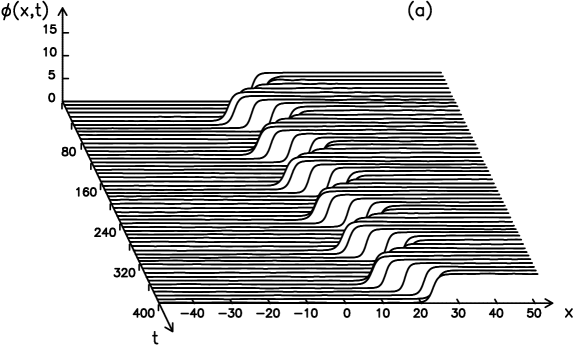
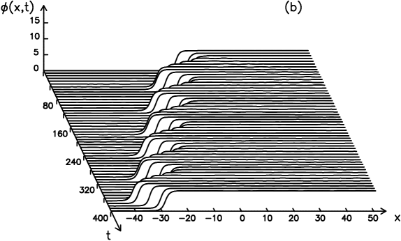
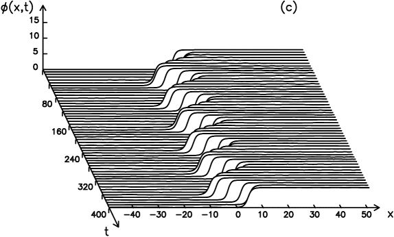
Figure 1: Verification of collective coordinate predictions in the absence of dissipation. Simulation starts from a kink with initial velocity $u(0)=0.5$ located at $X(0)=0$, and subject to an ac force given by $0.1\sin(0.1t+\delta_{0})$. (a) $\delta_{0}=0.75$, (b) $\delta_{0}=0$; notice that the direction of motion is opposite in both cases. (c) $\delta_{0}=0.6$, critical value exhibiting oscillatory motion.

Figure 2: Time evolution of the velocity of kink center mass. Parameter values as in Fig. 1. (a), (b) and (c) respectively. The solid curve shows the value of velocity, predicted by the collective coordinate perturbation [Eqs. (6,7)], and the dotted line is the numerical integration of [Eq. (1)]

.

3 Numerical results

Although the collective coordinate approach has been already tested very many times yo and is by now a standard technique to deal with soliton-bearing equations, the analytical expressions and the conclusions we have drawn from them should not be taken as valid before comparison with detailed and accurate numerical simulation of the full partial differential equation (1). To this end, we have numerically integrated it by means of a standard fourth order Runge-Kutta algorithm nrecipies with initial conditions given by an unperturbed sine-Gordon kink or breather with unrestricted initial velocity $u(0)$, and boundary conditions $\phi_{x}(L=\pm 50,t)=0$. We have carefully checked that our results did not depend on the choice of spatial and temporal steps, or the simulated system size (which can affect the simulations through the generation of spureous radiation).

We first address the validation of the results for kinks, beginning with the undamped case. In Fig. 1 we show the time evolution of a sG kink with initial velocity $u(0)=0.5$ (which is certainly far from being small) for different phases of the ac force $\delta_{0}$ and $\epsilon=0.1$, $\delta=0.1$. From Eq. (11) we know that the kink (with initial velocity $u(0)=0.5$) will oscillate only if $\delta_{0}=0.745$. Numerically, we searched for the critical phase of driving force and found $\delta_{0}=0.6$ (see Fig. 1c), i.e., the accuracy between these results it is of order of $0.1$. This is a very good prediction if we consider the value of the velocity and the value of $\epsilon$ (indeed, the accuracy is of the order of $\epsilon$ as should be expected). Note that there is practically no radiation visible in the simulations, which is in agreement with the correctness of the use of collective coordinate techniques. In connection with this, another interesting remark is that background motion, i.e., motion of the wings of the soliton induced by the ac force, is not visible in the simulations; this makes our approach very suitable for this problem, and as accurate as that of Olsen and Samuelsen olsam who introduced a term accounting for this negligible effect. We note that smaller initial velocities compare even better with our theoretical results. To appreciate to a larger extent the accuracy of our approach, Fig. 2 compares the analytical prediction for the velocity values [Eqs. (6,7)] with the velocity of the kink center of mass, obtained by integrating numerically Eq. (1). In these figures the parameters of the perturbed sG equation were chosen as in Fig. 1. We see from Fig. 2 that the agreement is excellent, in spite of the fact that the prediction of the critical velocity is not correct by a factor $\epsilon$. This is due, on one hand, to the fact that slight deviations from simmetry around $u(t)=0$ have dramatic consequences in the kink motion (note, e. g., Fig. 2c, the plot for the critical velocity, where the small discrepancy between the theory and the simulation is always in the same direction, towards negative $u$, corresponding to the theoretically predicted dc motion to the left), and, on the other hand, to the difficulties involved in numerically determining the critical velocity by checking that the kink just oscillates; this, among other things, depends on the integration time and on the time step. Hence, we believe that the correctness of our computations is much better appreciated by looking at the function $u(t)$ than simply verifying the critical velocity value.

We cannot close our study about sG kinks without providing numerical evidence that, as predicted by our analytical calculations above, it is not possible to induce dc motion on sG kinks by means of an ac force in the presence of damping. Figure 3 shows an example: a kink, initially moving with velocity $u(0)=0.5$, perturbed by ac force $0.01\sin(0.1t+0.1)$ and a damping term $\beta=0.05$, is stopped and ends up describing small amplitude oscillations around a finite region in space. This is but one example, although we must say that we have verified that our prediction is correct in very many other cases, with different choices of parameters, finding always an excellent agreement between analytics and numerics. As in the undamped case, Fig. 4, depicts the predicted and simulated motions of the kink center, exhibiting a perfect agreement between both. It is of course reasonable that the collective coordinate approach works better for the damped case, because if any radiation arises in the system, the damping wipes it away, leaving the kink as the only excitation present in the system, as the approximation requires.

Finally, for the breather case we present in Fig. 5 a comparison between the analytical and numerical threshold values of $\epsilon$ as a function of the initial frequency of the breather $\Omega_{0}$. We consider only the undamped case, $\beta=0$. We have observed in our simulations the phenomenon predicted by our analytical calculations: If the amplitude of the ac force exceeds the threshold value of $\epsilon$, the initial breather decomposes into a $k\bar{k}$ pair. As depicted in Fig. 5, the collective coordinate result predicts very well the threshold amplitude in all the range of breather frequencies, even for rather large values of such amplitude, where the perturbative approach might not work in principle. We note that, for driving frequencies close to 1 (the lower edge of the phonon band of the sG system), the breather can as well decay into radiation, but we have not pursued this process in detail in view of the difficulties involved in distinguishing breathers from linear radiation in this limit. Therefore, we concern ourselves with the decay into $k\bar{k}$ pairs, this being the reason we have not gone over $\Omega_{0}=0.9$ not in our numerical tests. Figure 6 shows an instance of our numerical determination of the threshold, for a breather with $\Omega_{0}=0.2$. We can see that if $\epsilon=0.0148$ (Fig. 6a) the frequency of the breather is modulated, but it remains a breather, as the oscillations of the field value at $x=0$ clearly show (of course, we have looked at the simulation over the whole spatial interval to confirm this). On the contrary, if we increase $\epsilon$ (for example, $\epsilon=0.0149$) then the breather breaks up into a $k\bar{k}$ pair (Fig. 6b), a phenomenon which reveals itself in the suppression of the oscillations at $x=0$ indicating that the breather stops its periodic motion. We have thus verified the validity of the collective coordinate results for the breather case as well.

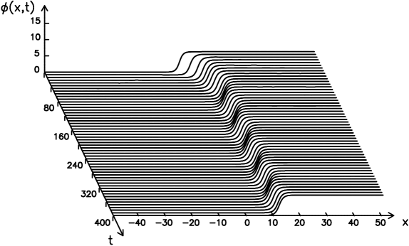
Figure 3: Verification of collective coordinate predictions with dissipation. This is one example of soliton motion, initially with velocity $u(0)=0.5$, and subject to an ac force given by $0.01\sin(0.1t+\delta_{0})$, with $\delta_{0}=0.1$ and $\beta=0.05$.

Figure 4: Time evolution of the velocity of kink center mass. Parameter values as in Fig. 3. The solid curve is the analytical prediction [Eqs. (12,13,14)] and the dotted curve is the numerical integration of [Eq. (1)].

Figure 5: Illustration of the threshold value of $\epsilon$ vs the initial frequency $\Omega_{0}$. Solid line represent the values given by the perturbation analysis and the points are the values, obtained by numerical simulation of perturbed sine-Gordon equation. The frequency and the phase of ac force are $\delta=0.1$, $\delta_{0}=0$ respectively.

Figure 6: (a) The breather with modulated frequency for the value of $\epsilon=0.0148$.(b) If $\epsilon=0.0149$ the breather break into $k\bar{k}$ pair. The others parameter values are $\Omega_{0}=0.2$, $\delta=0.1$, $\delta_{0}=0$. Compare with the analytical threshold $\epsilon$ ($\epsilon_{th}=0.0135$), obtained in Eqs. (25,26,27).

4 Conclusions

In this paper, we have shown both by analytical (collective coordinate theory) and numerical means the following three facts: i) Kink dc motion is possible in the sG system when forced by a pure ac force, except for a very special choice of the initial velocity related to the driving phase by equation (11); in this case, the kink center oscillates around its initial position; ii) kink dc motion induced by pure ac driving is never possible in the presence of damping, and iii) the undamped sG system forced by an ac driving allows the existence of breathers, whose frequency becomes modulated by the external one, up to a certain critical value of the amplitude that depends on the driving frequency and on the breather parameters. Above that amplitude, the breather decays to a kink-antikink pair.

As already stated, this findings arise from a perturbative calculation of the collective coordinate type, whose accuracy for very many soliton problems is well established yo . In this respect, we want to emphasize our main achievement in this study: We have proposed a change of variables which allows to linearize and fully solve the differential equation for the kink velocity without any restriction. We note that in previous works olsam ; anniu only the non-relativistic limit could be dealt with in an approximate manner. It is clear that this analytical procedure can be useful in similar equations, an example of this being our treatment of the long Josephson junction equation, with a more realistic dissipative term and a constant driving, in Appendix II. Therefore, having in mind the accuracy of the collective coordinate approach, the fact that there were no further approximations involved in our calculations, and the numerical confirmation of our predictions, we believe that our study settles down once and for all the question of kink motion in ac driven soliton bearing systems, particularly so for the sG equation.

From these results, which clarify the phenomenology of the ac driven sG equation, we can try to draw some more general conclusions on soliton-bearing problems perturbed by an ac force. The findings on discrete sG systems zaragoza suggest that for our conclusions to apply in other, different systems, it is necessary that the soliton or solitary wave under consideration does not have one or several internal oscillation modes which can be excited by the driving force. To check for the possible new phenomena or modifications of our conclusions coming from the existence of those modes, we have carried out some preliminary research on the ac driven $\phi^{4}$ model. Generally speaking, the same conclusions hold, i. e., in the absence of dissipation ($\beta=0$) the kink (antikink) will exhibit oscillatory motion if

$$\frac{u(0)}{\sqrt{1-u^{2}(0)}}=\pm[\frac{3\epsilon}{\sqrt{2}\delta}\cos\,(\delta_{0})],$$

whereas when dissipation is present we again find that kink dc motion is not possible. However, we have found numerical evidence that for values of the driving frequency close to the internal mode one, the kink behavior is much more complicated, even chaotic. We are currently working on understanding this effect analytically, and tentatively we relate it to the resonance of the driving and the internal mode physd . Similar resonance phenomena were observed for the sG kink in a harmonic potential well, when the driving had a frequency close to the natural one of the kink in the well fernandez , which reinforces our interpretation and expectations. This leads us to the conjecture that the results we have obtained for the sG problem can be true in general, provided as already said that there are no resonances with other modes intrinsic to the excitation. Of course, there also remains the question of drivings with frequencies above the phonon lower edge. We believe that our conclusions will still hold in that situation, in so far the presence of the external force does not cause an interaction between solitonic and radiation modes; it is to be expected that our calculations will be very accurate in the presence of dissipation, which will damp away any excited radiation. Finally, as shown in Appendix II below, we want to stress that the predictions and mathematical results we have obtained in this work have direct application in many physical systems, and among them in Josephson devices [more realistically described by Eq. (33) below]. It would be most interesting to verify the possibility of dc motion of solitons induced by pure ac driving in real systems like that, more so in view of the potential applications such a rectification effect might have. Another implication of our results has to do with soliton generation in systems described by sG equations: Indeed, by driving the system with an ac force strong enough, we could break up thermally created breathers into kink-antikink pairs, which under the influence of the driving would separate moving towards opposite directions. This would be a very simple and clean way of creating solitons in, e.g., Josephson devices. It thus becomes clear that experimental work pursuing this and related questions, which is certainly amenable with the present capabilities, would be most useful in assessing the importance of our work.

Appendix I

In this appendix we prove the necessary and sufficient condition for the sG soliton motion to be purely oscillatory in the presence of undamped ac driving. In the body of the paper we stated that this is so if and only if the condition (10), or equivalently, (11), takes place.

On the one hand, Substituting (11) in (7) and afterwards in (6) we obtain for the velocity function $u(t)$ the following expression:

$$u(t)=\frac{\pm{\frac{\pi\epsilon}{4\delta}}\cos(\delta t+\delta_{0})}{\sqrt{1+\left[{\frac{\pi\epsilon}{4\delta}}\cos(\delta t+\delta_{0})\right]^{2}}},$$ (28)

which can be integrated, yielding the position of the kink center of mass $X(t)$:

$$X(t)=X(0)\pm\frac{1}{\delta}\arcsin\left(\frac{\pi\epsilon\sin(\delta t+\delta_{0})}{\sqrt{16\delta^{2}+\pi^{2}\epsilon^{2}}}\right).$$ (29)

Hence, it is evident from the above equation that $X(t)$ is a periodic function with period $T={2\pi/\delta}$.

On the contrary, suppose that the kink center of mass

$$X(t)=\int_{0}^{t}{u(t^{\prime})}dt^{\prime}$$ (30)

oscillates with period $T={2\pi/\delta}$, i. e., $X(t)=X(t+T)$; this can be put as

$$I(a)\equiv\int_{t}^{t+T}{\frac{a+bcos(\delta t^{\prime}+\delta_{0})}{\sqrt{1+(a+bcos(\delta t^{\prime}+\delta_{0}))^{2}}}}dt^{\prime}=0,$$ (31)

where

$$a=\frac{u(0)}{\sqrt{1-u(0)^{2}}}\mp\frac{\pi\epsilon\cos(\delta_{0})}{4\delta}$$ (32)

and $b=\pi\epsilon/4\delta$. Noticing that, first $I(0)=0$; second, if $a<-|b|$ $I(a)<0$ and if $a>|b|$ $I(a)>0$, and third, $I^{\prime}(a)>0$ for all values of $a$, we arrive at the desired result that $I(a)=0$ if and only if the relation (11) [$a=0$] holds.

Appendix II

In McL realistic model of a long Josephson junction is proposed, given by the following perturbed sG equation

$$\phi_{tt}-\phi_{xx}+\sin(\phi)=-\beta\phi_{t}+\alpha\phi_{xxt}-\gamma,$$ (33)

where the term $\beta\phi_{t}$ represents the dissipation due tunneling of normal electrons across the barrier, $\alpha\phi_{xxt}$ is the dissipation caused by flow of normal electrons parallel to the barrier and $\gamma$ is a distributed bias current. In this appendix we apply our theory to this problem in order to show that our technique to solve the equation for the collective velocity can be applied to other problems. In addition, as the equation above is realized very approximately by actual Josephson devices, by studying it we will providing experimental means of checking our results as well as predicting behavior which might have an application of interest in that context.

To begin with, we note that if $\alpha=0$ this equation coincide with (1) letting $\delta=0$. Therefore, substituting $\delta=0$ and $\gamma=-\epsilon\sin(\delta_{0})$ in Eqs. (12,13,14) we obtain

$$u(t)=\frac{d_{0}\exp(-\beta t)+d}{\sqrt{1+(d_{0}\exp(-\beta t)+d)^{2}}},$$ (34)

where $d_{0}=u(0)/\sqrt{1-u(0)^{2}}-d$ and $d=\pm\pi\gamma/4\beta$. When $t$ goes to infinity, we have $u(\infty)\to d/\sqrt{1+d^{2}}$. Notice that this expression coincides with the equilibrium solution $u_{\infty}$, obtained in McL .

For $\alpha\neq 0$ the same procedure as above leads us to a first-order ordinary differential equation for $u(t)$, which is given by

$$\frac{du}{dt}=\pm\frac{\pi\gamma}{4}(1-u^{2})^{3/2}-\beta u(1-u^{2})-\frac{1}{3}\alpha u.$$ (35)

If we now introduce the same change of variable as in Sec. 2, $y(t)=u(t)/\sqrt{1-u(t)^{2}}$, Eq.  (35) becomes

$$\frac{dy}{dt}=\pm\frac{\pi\gamma}{4}-(\beta+\frac{\alpha}{3})y-\frac{1}{3}\alpha y^{3},$$ (36)

Integrating (36) we find

$$\frac{1}{p+x_{1}^{2}}\Bigg{\{}\ln\Bigg{(}c_{1}\frac{y-x_{1}}{\sqrt{\left(y+\frac{x_{1}}{2}\right)^{2}+k_{1}^{2}}}\Bigg{)} -$$

$$-\frac{3x_{1}}{2k_{1}}\left[\arctan\left(\frac{y+\frac{x_{1}}{2}}{k_{1}}\right)-c_{2}\right]\Bigg{\}} = -\alpha t,$$ (37)

where

$$3p = \frac{3\beta}{\alpha}+1$$ (38)

$$2q = \mp\frac{3\pi\gamma}{4\alpha}$$ (39)

$$D = q^{2}+p^{3},$$ (40)

$$x_{1} = (\sqrt{D}-q)^{1/3}-\frac{p}{(\sqrt{D}-q)^{1/3}},$$ (41)

$$k_{1}^{2} = 3p+\frac{3}{4}x_{1}^{2},$$ (42)

$$c_{1} = \frac{\sqrt{(y(0)+\frac{x_{1}^{2}}{2})^{2}+k_{1}^{2}}}{y(0)-x_{1}},\mbox{ and}$$ (43)

$$c_{2} = \arctan\left(\frac{y(0)+\frac{x_{1}}{2}}{k_{1}}\right).$$ (44)

For large values of $t$, $y(\infty)\to x_{1}$, so the kink will move with constant velocity $u(\infty)\to\frac{x_{1}}{\sqrt{1+x_{1}^{2}}}$, which depends on the parameters $\alpha$, $\beta$ and $\gamma$. For example, if $\gamma=0$ ($q=0$), $\displaystyle u(t)|_{t\to\infty}=0$, i.e. by the influence of both dissipation terms ($-\beta\phi_{t}$ and $\alpha\phi_{xxt}$) the kink will be stopped.

References

- (1) M. Remoissenet, Waves called solitons (Springer, Berlin-Heidelberg, 1994).
- (2) A. Sánchez and A. R. Bishop, SIAM Review, in press (1998).
- (3) Yu. S. Kivshar and B. A. Malomed, Rev. Mod. Phys. 61, 763 (1989).
- (4) A. Sánchez and L. Vázquez, Int. J. Mod. Phys. B 5, 2825 (1991).
- (5) Most important in contexts where soliton stability is a crucial factor, as it happens in many applications (Josephson junctions, fiber optics). Dynamical solitons are easy much more sensitive to perturbations; an archetypal example are those of the Korteweg-de Vries equation (see, e.g, km and references therein).
- (6) G. L. Lamb, Rev. Mod. Phys. 43, 99 (1971).
- (7) T. H. R. Skyrme, Proc. Roy. Soc. London A247, 260 (1958).
- (8) T. H. R. Skyrme, Proc. Roy. Soc. London A262, 237 (1961).
- (9) U. Enz, Phys. Rev. 131, 1392 (1963).
- (10) R. Rajaraman, Solitons and Instantons (North-Holland Publishing Company, Amsterdam, 1982).
- (11) A. Barone and G. Paternó, Physics and applications of the Josephson effect (Wiley, New York, 1982).
- (12) E. Feldtkeller, Phys. Stat. Sol. 27, 161 (1968).
- (13) J. D. Weeks and G. H. Gilmer, Adv. Chem. Phys. 40, 157 (1979).
- (14) A. Sánchez, D. Cai, N. Grønbech-Jensen, A. R. Bishop, and Z. J. Wang, Phys. Rev. B 51, 14 664 (1995).
- (15) J. Frenkel and T. Kontorova, J. Phys. USSR, 1, 137 (1939).
- (16) F. R. N. Nabarro, Theory of crystal dislocations (Dover, New York, 1987).
- (17) C. Cattuto and F. Marchesoni, Phys. Rev. Lett. 79, 5070 (1997).
- (18) S. W. Englander, N. R. Kallenbach, A. J. Heeger, J. A. Krumhansl and S. Litwin, Proc. Natn. Acad. Sci. USA 77, 7222 (1980).
- (19) M. Salerno, Phys. Rev. A 44, 5292 (1991).
- (20) L. V. Yakushevich, Reviews of Biophysics 26, 201 (1993).
- (21) L. V. Yakushevich, Studia Biophysica 121, 201 (1987).
- (22) P. J. Pascual and L. Vázquez, Phys. Rev. B 32, 8305 (1985).
- (23) A. Sánchez, A. R. Bishop and F. Domínguez-Adame, Phys. Rev. E 49, 4603 (1994).
- (24) D. Cai, A. R. Bishop and A. Sánchez, Phys. Rev. E 48, 2, 1447 (1993).
- (25) M. B. Fogel, S. E. Trullinger, A. R. Bishop and J. A. Krumhansl, Phys. Rev. B 15, 1578 (1977).
- (26) D. W. McLaughlin and A. C. Scott, Phys. Rev. A 18, 1652 (1978).
- (27) P. S. Lomdahl, O. H. Olsen and M. R. Samuelsen, Phys. Rev. A 29, 350 (1984).
- (28) J. C. Ariyasu and A. R. Bishop, Phys. Rev. B 35, 3207 (1987).
- (29) D. W. McLaughlin and E. A. Overman, Phys. Rev. A 26, 3497 (1982).
- (30) P. S. Lomdahl and M. R. Samuelsen, Phys. Rev. A. 34, 664 (1986).
- (31) P. S. Lomdahl and M. R. Samuelsen, Phys. Lett. A. 128, 427 (1988).
- (32) O. H. Olsen and M. R. Samuelsen, Phys. Rev. B 28, 210 (1983).
- (33) L. L. Bonilla and B. A. Malomed, Phys. Rev. B 43, 11 539 (1991).
- (34) D. Cai, A. Sánchez, A. R. Bishop, F. Falo and L. M. Floría, Phys. Rev. B 50, 9652 (1992).
- (35) P. J. Martínez, F. Falo, J. J. Mazo, L. M. Floría and A. Sánchez, Phys. Rev. B 56, 87 (1997).
- (36) N. R. Quintero and A. Sánchez, preprint cond-mat/9709063, Phys. Lett. A, to appear.
- (37) A. R. Bishop, D. W. McLaughlin and M. Salerno, Phys. Rev. A 40, 6463 (1989).
- (38) W. H. Press, S. A. Teukolsky, W. T. Vetterling and B. P. Flannery, Numerical Recipes in Fortran 2nd Edition (Cambridge University Press, Cambridge, 1992).
- (39) For , the last point in Fig. 6, the breather does decay into radiation instead of a into kink-antikink pair. We have included this point in the plot because in this case we could make sure that the breather had indeed disappeared.
- (40) N. R. Quintero, A. Sánchez, and F. Domínguez-Adame, Resonances, bifurcations, and kink dc motion in the ac driven equation, to be published.
- (41) J. C. Fernández, M. J. Goupil, O. Legrand, and G. Reinisch, Phys. Rev. B 34, 6207 (1986).