Fractional Populations in Sex-linked Inheritance

Abstract

We study the fractional populations in chromosome inherited diseases. The governing equations for the fractional populations are found and solved in the presence of mutation and selection. The physical fixed points obtained are used to discuss the cases of color blindness and hemophilia.

I Introduction

Many physical ideas are finding applications in complex biological systems these days[1, 2]. Recently, we presented a theoretical scheme in which one can investigate the ratios between the fractional population of blood groups[3]. This method has some analogy with the physical concept of renormalization and fixed points. In this paper, we extend the theory to investigate the problem of sex-linked inheritance.

In sex-linked inheritance, there are five population groups, $XX$, $X^{\prime}X$, $X^{\prime}X^{\prime}$, $XY$, and $X^{\prime}Y$, where $X$, $X^{\prime}$ and $Y$ represent the normal female, the defective female, and the male chromosome, respectively. The group of so called carrier female is characterized by $X^{\prime}X$. The genetic rule is that sons receive $Y$ and daughters do $X$ or $X^{\prime}$ from their fathers. Similarly, their mothers deliver $X$ or $X^{\prime}$ to sons and daughters. It is also known that there exist mutations between $X$ and $X^{\prime}$. Another important factor in the present problem is that the defective groups, $X^{\prime}X^{\prime}$ and $X^{\prime}Y$, have disadvantages in surviving and inheriting unlike in the case of the blood groups[3]. This selection process should be taken into account for any reasonable discussions. Therefore, we consider the inheritance of sex-linked disease in the presence of mutation and selection and obtain the governing equations, which determine the next fractional populations from the previous ones. The governing equations will be used to investigate the problems of genetic propagations of chromosome-linked diseases such as color blindness and hemophilia.

II fractional population equations

We consider the five fractional populations with the following constraints:

$$XX(n)+X^{\prime}X(n)+X^{\prime}X^{\prime}(n)=1$$ (1)

$$XY(n)+X^{\prime}Y(n)=1,$$ (2)

for the $n$-th generation. The ratios of gene frequencies without mutation can be determined as

$$\widetilde{X_{f}}(n) = XX(n)+\frac{1}{2}X^{\prime}X(n),$$ (3)

$$\widetilde{X_{f}^{\prime}}(n) = X^{\prime}X^{\prime}(n)+\frac{1}{2}X^{\prime}X(n),$$ (4)

$$\widetilde{X_{m}}(n) = XY(n),$$ (5)

$$\widetilde{X_{m}^{\prime}}(n) = X^{\prime}Y(n).$$ (6)

Although the mutation between the normal chromosome $X$ and the defective one $X^{\prime}$ would be rare, still it plays an important role in the following discussion. In order to consider the mutation, we introduce two probability factors, $\alpha$ and $\beta$ for the following mutation processes;

$$X\stackrel{{\scriptstyle\alpha}}{{\longrightarrow}}X^{\prime}\qquad\mbox{and}\qquad X\stackrel{{\scriptstyle\beta}}{{\longleftarrow}}X^{\prime}.$$ (7)

Through the above mutation processes, the gene frequencies are modified as

$$X_{f}(n) = (1-\alpha)\widetilde{X}_{f}(n)+\beta\widetilde{X}_{f}^{\prime}(n),$$ (8)

$$X_{f}^{\prime}(n) = (1-\beta)\widetilde{X}_{f}^{\prime}(n)+\alpha\widetilde{X}_{f}(n),$$ (9)

$$X_{m}(n) = (1-\alpha)\widetilde{X}_{m}(n)+\beta\widetilde{X}_{m}^{\prime}(n),$$ (10)

$$X_{m}^{\prime}(n) = (1-\beta)\widetilde{X}_{m}^{\prime}(n)+\alpha\widetilde{X}_{m}(n).$$ (11)

The fractional population equations, which govern the populations of the next generation, are now written as

$$\widetilde{XX}(n+1) = X_{f}(n)\times X_{m}(n),$$ (12)

$$\widetilde{X^{\prime}X}(n+1) = X_{f}^{\prime}(n)\times X_{m}(n)+X_{f}(n)\times X_{m}^{\prime}(n),$$ (13)

$$\widetilde{X^{\prime}X^{\prime}}(n+1) = X_{f}^{\prime}(n)\times X_{m}^{\prime}(n),$$ (14)

$$\widetilde{XY}(n+1) = X_{f}(n),$$ (15)

$$\widetilde{X^{\prime}Y}(n+1) = X_{f}^{\prime}(n).$$ (16)

Since the defective chromosome causes a disease, the populations of $\widetilde{X^{\prime}X^{\prime}}$ and $\widetilde{X^{\prime}Y}$ will have less chances of surviving and inheriting their genes. In order to reflect this disadvantages, we introduce disadvantage factors $\delta_{f}$ for the female and $\delta_{m}$ for the male groups, respectively. Then, the populations of $\widetilde{X^{\prime}X^{\prime}}$ and $\widetilde{X^{\prime}Y}$ will be modified as

$$\mbox{Pop}[\widetilde{X^{\prime}X^{\prime}}(n+1)] \longrightarrow (1-\delta_{f})\mbox{Pop}[\widetilde{X^{\prime}X^{\prime}}(n+1)],$$ (17)

$$\mbox{Pop}[\widetilde{X^{\prime}Y}(n+1)] \longrightarrow (1-\delta_{m})\mbox{Pop}[\widetilde{X^{\prime}Y}(n+1)].$$ (18)

With normalization, the fractional population equations are given by

$$XX(n+1) = \frac{X_{f}(n)\cdot X_{m}(n)}{1-\delta_{f}X_{f}^{\prime}(n)\cdot X_{m}^{\prime}(n)},$$ (19)

$$X^{\prime}X(n+1) = \frac{X_{f}^{\prime}(n)\cdot X_{m}(n)+X_{f}(n)\cdot X_{m}^{\prime}(n)}{1-\delta_{f}X_{f}^{\prime}(n)\cdot X_{m}^{\prime}(n)},$$ (20)

$$X^{\prime}X^{\prime}(n+1) = \frac{(1-\delta_{f})X_{f}^{\prime}(n)\cdot X_{m}^{\prime}(n)}{1-\delta_{f}X_{f}^{\prime}(n)\cdot X_{m}^{\prime}(n)},$$ (21)

$$XY(n+1) = \frac{X_{f}(n)}{1-\delta_{m}X_{f}^{\prime}(n)},$$ (22)

$$X^{\prime}Y(n+1) = \frac{(1-\delta_{m})X_{f}^{\prime}(n)}{1-\delta_{m}X_{f}^{\prime}(n)}.$$ (23)

The above governing equations (1)$\sim$(19) yield the following constraint relations for any generation $n$,

$$X_{f}(n)+X_{f}^{\prime}(n)=1\qquad\mbox{and}\qquad X_{m}(n)+X_{m}^{\prime}(n)=1.$$ (24)

In order to understand the change of populations along generations, it is convenient to consider the automata equations for $X_{f}^{\prime}$ and $X_{m}^{\prime}$ only, which are given by

$$X_{m}^{\prime}(n+1) = \frac{\alpha+\left(1-\alpha-\beta-\delta_{m}(1-\beta)\right)X_{f}^{\prime}(n)}{1-\delta_{m}X_{f}^{\prime}(n)},$$ (25)

$$2X_{f}^{\prime}(n+1) = \frac{2\alpha+(1-\alpha-\beta)\left(X_{f}^{\prime}(n)+X_{m}^{\prime}(n)\right)-2\delta_{f}(1-\beta)X_{f}^{\prime}(n)\cdot X_{m}^{\prime}(n)}{1-\delta_{f}X_{f}^{\prime}(n)\cdot X_{m}^{\prime}(n)}.$$ (26)

The above coupled recursion relations can now be used to study the fixed points of $X_{m}^{\prime}$ and $X_{f}^{\prime}$, which correspond to the equilibrium values where $X_{m}^{\prime}(n+1)=X_{m}^{\prime}(n)={X_{m}^{\prime}}^{\ast}$ and $X_{f}^{\prime}(n+1)=X_{f}^{\prime}(n)={X_{f}^{\prime}}^{\ast}$. The fixed points of ${X_{f}^{\prime}}^{\ast}$ are given by the solutions of the algebraic equation,

$$a_{0}+a_{1}{X_{f}^{\prime}}^{\ast}+a_{2}({X_{f}^{\prime}}^{\ast})^{2}+a_{3}({X_{f}^{\prime}}^{\ast})^{3}=0,$$ (27)

where the coefficients $a_{i}$ are given by

$$a_{0} = \alpha(3-\alpha-\beta),$$ (28)

$$a_{1} = (\alpha+\beta)(\alpha+\beta-3)+\delta_{m}(2\beta-\alpha-\beta^{2}-\alpha\beta-1)+2\delta_{f}\alpha(\beta-1),$$ (29)

$$a_{2} = \delta_{m}(1+\alpha+\beta)+2\delta_{f}(2\alpha+2\beta-\beta^{2}-\alpha\beta-1)+2\delta_{m}\delta_{f}(\beta-1)^{2},$$ (30)

$$a_{3} = 2\delta_{f}(1-\alpha-\beta)+2\delta_{m}\delta_{f}(\beta-1).$$ (31)

Solving this equation for stable fixed points, we can readily determine the equilibrium population ratios.

We study the fixed points in several cases. First of all, in the case of no mutation; $\alpha=0$ and $\beta=0$, the meaningful fixed point, ${X_{f}^{\prime}}^{\ast}$, is given by 0. It correctly predicts that without mutations, the defective genes will disappear eventually. Secondly, when only mutations are considered in the theory assuming $\delta_{m}=0$ and $\delta_{f}=0$, the fixed point is given by ${X_{f}^{\prime}}^{\ast}=\alpha/(\alpha+\beta)$. This result will be used in the discussion for color blindness. In other general cases, the exact solution cannot be expressed in a closed form. However, since the mutation rates are known to be very small($\sim 10^{-5}\sim 10^{-7}$), the fixed point ${X_{f}^{\prime}}^{\ast}$ can be expressed in terms of $\alpha$ and $\beta$ in an approximate fashion and will be discussed in the next section.

III color blindness and hemophilia

The disadvantage, that a color blindness man or woman has, is not severe enough to reduce the chance of survival significantly. Hence, we let the disadvantage factors be simply zero in this case. Then, we easily notice from Eq. (25) that the fixed point is given by

$${X_{m}^{\prime}}^{\ast}={X_{f}^{\prime}}^{\ast}=\frac{\alpha}{\alpha+\beta}.$$ (32)

This result is identical to that obtained in the conventional genetics[4].

Using the fractional population equations of Eq. (19) and the above fixed point, we obtain the population ratios as

$$XY:X^{\prime}Y=X_{f}^{\ast}:{X_{f}^{\prime}}^{\ast}=1-{X_{f}^{\prime}}^{\ast}:{X_{f}^{\prime}}^{\ast}=\beta:\alpha,$$ (33)

and furthermore

$$XX:X^{\prime}X:X^{\prime}X^{\prime}=\beta^{2}:2\beta\alpha:\alpha^{2}.$$ (34)

The above result is the well known the Hardy-Weinberg law[5].

The demographic data for color blindness in England show that $XY:X^{\prime}Y=12:1$[6]. Hence we conclude that $\beta:\alpha=12:1$. We notice that $X^{\prime}$ chromosome is more unstable than $X$ chromosome since $\beta$ is much larger than $\alpha$. The abundance of carrier female is easily noticed by the fact that $XX:X^{\prime}X:X^{\prime}X^{\prime}=144:24:1$.

Hemophilia is a dreadful disease which affects the chance of survival and mating significantly. All of the female group $X^{\prime}X^{\prime}$ perish completely upon birth. Hence, the disadvantage factor $\delta_{f}$ is equal to 1. Then the fixed point ${X_{f}^{\prime}}^{\ast}$ can be expressed up to the second order of $\alpha$ and $\beta$ as follows using Eq. (27) and (28),

$${X_{f}^{\prime}}^{\ast} = \frac{3}{\delta}_{m}\alpha+\left(-\frac{4}{\delta}_{m}+\frac{12}{\delta_{m}^{2}}-\frac{18}{\delta_{m}^{3}}\right)\alpha^{2}+\left(\frac{5}{\delta}_{m}-\frac{9}{\delta_{m}^{2}}\right)\alpha\beta+{\cal O}(\alpha^{3},\alpha^{2}\beta,\alpha\beta^{2},\beta^{3}),$$ (35)

$${X_{m}^{\prime}}^{\ast} = (-2+\frac{3}{\delta}_{m})\alpha+\left(-2-\frac{10}{\delta_{m}}+\frac{30}{\delta_{m}^{2}}-\frac{18}{\delta_{m}^{3}}\right)\alpha^{2}+\left(-2+\frac{11}{\delta_{m}}-\frac{9}{\delta_{m}^{2}}\right)\alpha\beta+{\cal O}(\alpha^{3},\cdots).$$ (36)

A numerical calculation of the stable fixed point, ${X_{f}^{\prime}}^{\ast}$ using Eq. (27) is shown in Fig. 1. We find that the dominant contributions come from $\alpha$ and $\delta_{m}$ as Eq. (35) indicates. We also find that the values of the fixed point ${X_{f}^{\prime}}^{\ast}$ are independent of initial values. The approximate expressions, Eqs. (35) and (36) are found in good agreement with the exact expression Eq. (27) except when $\delta_{m}$ is near zero.

It is useful to consider the male hemophilia population before selection in order to relate the above formulation with the statistical data. Here, the relevant demographic data is the ratio, $r$, between the mutation cases and the all hemophilia cases; $\widetilde{X^{\prime}Y}^{\ast}_{mut}=r\cdot\widetilde{X^{\prime}Y}^{\ast}$. Using Eqs. (3)$\sim$(19), the population of male infants with hemophilia before selection can be written as

$$\widetilde{X^{\prime}Y}^{\ast}=\frac{1}{2}(1+\alpha-\beta)X^{\prime}X^{\ast}+\alpha XX^{\ast}\equiv\widetilde{X^{\prime}Y}^{\ast}_{inh}+\widetilde{X^{\prime}Y}^{\ast}_{mut}.$$ (37)

Here, the second term represents the male population having hemophilia caused by the spontaneous gene mutation. Actually, the first term also contains the gene mutation contribution of $\frac{1}{2}(\alpha-\beta)X^{\prime}X^{\ast}$. However, when the demographic data $r$ are collected, there is no way to distinguish the inheritance from the mutation in this case, because data collectors simply check whether there were hemophiliac occurrences in the family line or not. It is straightforward to show that $r$ is related to the disadvantage factor $\delta_{m}$ and the mutation rates $\alpha$ and $\beta$. From Eqs. (3)$\sim$(19), we find

$$\delta_{m}=3r+(10-10r-\frac{2}{r})\alpha+(-3+5r)\beta+{\cal O}(\alpha^{2},\alpha\beta).$$ (38)

The early statistical data for the infant male population having hemophilia[7] show that $\widetilde{XY}:\widetilde{X^{\prime}Y}\simeq 10^{4}:1$. Assuming that the current fractional population distribution has reached a fixed point, we find ${X_{f}^{\prime}}^{\ast}\simeq 10^{-4}$ from Eq. (12). Furthermore, a recent statistics shows that the rate $r$ is given by $r\simeq\frac{1}{3}$[8]. This data and Eq. (38) yield $\delta_{m}=1-{\cal O}(\alpha,\beta)$. This result is in a reasonable agreement with the fact that various therapies treating male hemophilia have been invented only recently and, thus, the probability of successful marriage and reproduction was almost zero for male patient in the past. With $\delta_{m}\simeq 1$ and ${X_{f}^{\prime}}^{\ast}\simeq 10^{-4}$, we find from Eq. (35) that the value of $\alpha$ is about $3.3\times 10^{-5}$, which is in a reasonable range as the probability of mutation. Also, we can obtain the population ratio of the carrier female group using Eq. (19); $XX:X^{\prime}X:X^{\prime}X^{\prime}\sim 10^{4}:1.33:0$.

Since the level of therapies treating male hemophilia has now reached the stage that most of male patient can marry and reproduce, it is interesting to study the case $\delta_{m}=0$ and make predictions how the mutation rate and the fractional population will change accordingly. The fixed point of Eq. (35) and (36) will be modified as

$${X_{f}^{\prime}}^{\ast} = \sqrt{\frac{3}{2}}\alpha^{\frac{1}{2}}+{\cal O}(\alpha,\cdots),$$ (39)

$${X_{m}^{\prime}}^{\ast} = \alpha+(1-\alpha+\beta){X_{f}^{\prime}}^{\ast}.$$ (40)

Using the above results, we find the modified rate

$$r=\sqrt{\frac{2}{3}}\alpha^{\frac{1}{2}}+{\cal O}(\alpha,\cdots).$$ (41)

Assuming the mutation rate $\alpha$ does not change and remain $\alpha\simeq 3.3\times 10^{-5}$ as we find in the above, we can determine ${X_{f}^{\prime}}^{\ast}=0.00707$. Also, we readily obtain the fractional populations: $XX:X^{\prime}X:X^{\prime}X^{\prime}=98.6:1.41:0$, and $XY:X^{\prime}Y=993:7$. The result clearly shows that the majority of hemophilia would results from inheritance and that the fractional population of carrier female increases drastically, when male hemophiliac patients survive and mate without any disadvantages. Therefore, nongenetic treatment of hemophiliac male may cause increase of hemophiliac population and infant deaths of female patients, unless some concurrent measures are taken. However, we note that the present calculation can not produce the dynamic properties of the transition period between $\delta_{m}\simeq 1$ and $\delta_{m}\simeq 0$, since $\delta_{m}$ is assumed static in the calculation.

IV conclusion

We have considered the population ratios of the genetic groups related with chromosome inherited diseases. The governing equations, which determine the ratios, are found in the presence of mutation and selection. The selection is taken into account in the formulation by using the disadvantage factors. It is found that there exist physical fixed points in the automata equations, which correspond to equilibrium population rates. These fractional population equations are used to discuss the cases of color blindness and hemophilia.

In the case of color blindness, there is no significant disadvantage in selection so that the disadvantage factors can be assumed zero. From the governing equations, we readily obtain the Hardy-Weinberg relation $XX:X^{\prime}X:X^{\prime}X^{\prime}=\beta^{2}:2\alpha\beta:\alpha^{2}$. Using the statistical data $XY:X^{\prime}Y=12:1$, we find that the ratio of mutation rates $\alpha:\beta=1:12$.

Hemophilia seriously hampers chances of survival, mating and reproduction. Especially for female patients, chance of survival is almost zero, thus, making $\delta_{f}=1$. Using the demographic data that one out of ten thousand male infants have hemophilia, and that one third of all hemophiliac cases are thought to be caused by gene mutation, we obtain the following results; i) the disadvantage factor $\delta_{m}$ for male is almost 1, ii) the mutation rate $\alpha\simeq 3.3\times 10^{-5}$, and iii) $XX:X^{\prime}X\simeq 10^{4}:1.33$.

We have also studied the case when the hemophiliac male suffers no disadvantage in the selection process; $\delta_{m}=0$. It is found that the population of hemophiliac females and males would increase drastically and inheritary hemophilia would be dominant over gene mutated cases.

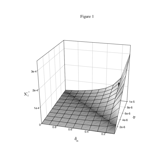
FIG. 1.: For a set of values of $\delta_{f}=0.5$ and $\beta=10^{-5}$, we plot the fixed point ${X_{f}^{\prime}}^{\ast}$ in the three dimensional format, where the $x$ and $y$-axis correspond the mutation rate $\alpha$ and the male disadvantage factor $\delta_{m}$. It is found that the overall features of the shape and size do not depend on $\delta_{f}$ and $\beta$ sensitively.

REFERENCES

• [1] A. S. Perelson and G. Weisbuch, Rev. Mod. Phys. 69, 1219(1997).
• [2] D. A. Z. Mekjian, Phys. Rev. A44, 8361(1991).
• [3] M.-H. Chung, S. P. Lee, C. K. Kim, and K. Nahm, Phys. Rev. E56, 865 (1997).
• [4] See e.g., P. W. Hedrick, Genetics of Populations, (Jones And Bartlett Publishers, Inc., Boston, 1985).
• [5] C. C. Li, First Course in Population Genetics, (Boxwood, Pacific Grove, CA, 1976).
• [6] T. Strachan and A. P. Read, Human Molecular Genetics, (Bios Scientific Publishers, 1996).
• [7] I. H. Porter, Heredity and disease, (McGraw-Hill, New York, 1968), pp.212-214.
• [8] http://www.hemophilia.org/bleeding-info/hemophilia/hemo.html