Directed Ising type dynamic preroughening transition in one dimensional interfaces

Abstract

We present a realization of directed Ising (DI) type dynamic absorbing state phase transitions in the context of one-dimensional interfaces, such as the relaxation of a step on a vicinal surface. Under the restriction that particle deposition and evaporation can only take place near existing kinks, the interface relaxes into one of three steady states: rough, perfectly ordered flat (OF) without kinks, or disordered flat (DOF) with randomly placed kinks but in perfect up-down alternating order. A DI type dynamic preroughening transition takes place between the OF and DOF phases. At this critical point the asymptotic time evolution is controlled not only by the DI exponents but also by the initial condition. Information about the correlations in the initial state persists and changes the critical exponents.

I Introduction

Absorbing type dynamic phase transitions are the focus of extensive research [1, 2, 3, 4, 5, 6, 7, 8, 9, 10, 11, 12]. These transitions occur in dynamic processes with trapped states. At the absorbing side of the phase transition, the system evolves into one specific microscopic state, a so-called absorbing state, out of which it can not escape. At the active side of the phase transition, the system manages to avoid such traps. An ensemble has a finite probability to stay alive.

Two distinct types of absorbing phase transitions have been identified in one dimension: the directed percolation (DP) and directed Ising (DI) universality class. DP type dynamic critical behavior has been found in, e.g., Schlögl’s first model for contact processes [2, 3], pair contact processes [4], and branching annihilating random walks (BAW) with an odd-number of offspring [5]. DI type dynamic critical behavior has been found in, e.g., probabilistic cellular automata [6], nonequilibrium kinetic Ising type models [7], interacting monomer-dimer models [8], and BAW models with an even-number of offspring [5, 9]. These models describe a wide range of phenomena, in particular epidemic spreading and catalytic chemical reactions.

In analogy with equilibrium phase transitions, it is believed that dynamic universality classes are determined by the degeneracy and symmetries of the absorbing states and by the symmetry properties of interfaces (domain walls) between them [10, 11, 12]. DP type transitions involve typically only a single absorbing state or a set of absorbing states with one of them dynamically more prominent in a coarse grained sense than the others [4, 10, 12]. DI type transitions involve two equivalent adsorbing states or two equivalent classes of absorbing states [13].

Counting the number of absorbing states is not sufficient. The degeneracy of the absorbing states can be obscured by the formulation of the dynamic rule. For example, in BAW dynamics involving only one species of particles, the “empty” absorbing state seems not to be degenerate, but the transition belongs to the DI universality class if the dynamics conserves the particle number modulo 2 [5, 9]. In that case particles can be reinterpreted as domain walls and we can color the domains at opposite sides of the walls alternatingly with two colors. One of the two colors dies out in the adsorbing state. This is reminiscent of the domain wall formulation of the equilibrium Ising model, where the existence of two coexisting phases is also obscured.

One appealing scheme of classifying absorbing phase transitions is by association with conventional equilibrium phase transitions. For example, consider the one-dimensional Ising model with single spin-flip dynamics. In terms of domain walls this involves the following processes: spontaneous creation of domain wall pairs $0\to 2A$ with probability $p_{sp}$ (the Boltzmann weight), hopping of single domain walls with probability $p_{h}=1$, and pair annihilation $2A\to 0$ with probability $p_{a}=1$. The stationary state of this model is the equilibrium state, which is obviously “disordered” (active) in one dimension. However, the model evolves always into one of the two perfectly ordered (absorbing) states if we disallow the spontaneous creation of domain walls, $p_{sp}=0$, because then the domain wall density can only decrease. The DI transition comes into play when branching processes are allowed; i.e., the creation of domain wall pairs in the vicinity of existing domain walls, $A\to 3A$. Branching can keep the system alive, while the two perfectly ordered Ising ground states still remain absorbing states. The resulting model is known as the BAW model with two offspring.

The same line of reasoning associates a distinct absorbing type dynamic universality class with each conventional equilibrium universality class, like the familiar $q$-state Potts and $q$-state clock universality classes. However, none of the models studied thus far with higher symmetries than the Ising model has an absorbing phase transition. Dynamic processes with more than 2 equivalent absorbing states $(q\geq 3)$ appear to be always active [11, 14]. Cardy and Täuber provide a possible explanation for this [15]. Additional systematic numerical studies are needed to settle this issue.

In this paper we introduce an application of absorbing phase transitions to the dynamics of one-dimensional solid-gas interfaces. We find a one-dimensional dynamic preroughening (PR) transition from an ordered flat (absorbing) phase to a disordered flat (active) phase. Consider the one-dimensional restricted solid-on-solid (RSOS) model description of crystal surfaces. The height difference between nearest neighboring columns of particles is 0 or $\pm 1$, i.e., only steps (kinks) with single atomic heights are allowed. A conventional dynamic Monte Carlo type equilibration process where single particles adsorb on or desorb from the surface with equal probability leads to a rough equilibrium surface with Edwards-Wilkinson (EW) type [16] scaling properties. In analogy with the above directed Ising model discussion, we transform the perfectly ordered flat state into an absorbing state by disallowing adsorption and desorption of particles at flat segments of the surface (spontaneous creation of step pairs). The only processes allowed are: hopping/pair annihilation of steps by adsorbing or desorbing a particle at step edges and branching of steps by adsorption or desorption at the next nearest neighbour sites near existing steps. The branching processes fall into two classes: the ones that preserve local flatness and those that create local roughness. We give them independent probabilities.

This model describes the evolution of the one dimensional interface from any initial random rough configuration to three types of stationary states: a rough phase with dynamic exponent $z=2$ (EW type), a perfectly ordered flat (OF) absorbing phase without steps, and an active disordered flat (DOF) phase. DOF phases are well known in equilibrium surfaces. They represent step liquids where the surface remains flat due to long-range step-up step-down alternating order but steps are placed randomly [17, 18]. Our dynamic DOF stationary state has no defects, i.e., the up-down alternating order is perfect and the the steps are placed randomly.

Although the dynamic DOF phase is active, it has an absorbing state type property. The OF absorbing state and the DOF active phase at the other side of the transition have in common that both “ground states” lack thermodynamic defects (both are at their fixed point in the sense of renormalization theory).

Equilibrium preroughening transitions belong to the Ashkin-Teller universality class [17, 18]. They involve two coupled Ising type order parameters. They are non-zero at opposite sides of the transition. A perfectly DOF initial configuration has a half integer average surface height $n+\frac{1}{2}$ and evolves at the OF side of the PR transition into a perfectly flat ordered absorbing state with $n$ or $n+1$ integer surface height. This OF-type two-fold degeneracy is the conventional spontaneous symmetry breaking associated with DI type transitions. However, an Ising type degeneracy exists also at the DOF side of the PR transition. An initial state with an integer average surface height $n$, evolves into a stationary DOF state with surface height $n+\frac{1}{2}$ or $n-\frac{1}{2}$. We call this the DOF-type degeneracy. In analogy with equilibrium transitions one might expect therefore that the dynamic PR transition be described by 2 coupled DI transitions. This turns out not to be the case.

The dynamic PR transition belongs to the (single) DI universality class. The two types of spontaneous symmetry breaking are not on an equal footing. A perfect DOF initial state can decay into the OF state, but a perfect OF state is frozen forever (even at the DOF side of the PR transition). The DOF type degeneracy does not create additional DI critical fluctuations. But it still affects the scaling behaviour. Configurations with perfect DOF order form an invariant subspace (which includes the OF ordered state). As shown below, this leads to a peculiar initial configuration dependence of the asymptotic decay of the step densities (the kinks in the one-dimensional interface).

In section 2, we introduce our model in detail. It is instructive to interpret it not only as a model for surface relaxation, but also for surface catalysis. In its latter reincarnation, the process is a two-species generalization of the BAW model with two offspring. The up and down steps (kinks) represent two species of particles, $A$ and $B$.

In section 3 we limit ourselves to configurations with perfect $ABAB$ alternating order. These DOF type configurations form a dynamical invariant subspace. The numerical results presented in section 3 confirm that our PR transition belongs to the DI universality class.

In section 4, we discuss the crossover scaling properties of the DI critical point into the rough phase. The rough phase has conventional EW type scaling properties. Recall that we disallow spontaneous adsorption and desorption from flat surface segments; surface roughness can only be created and maintained by branching. Apparently, this restriction does not alter the scaling properties of the rough phase.

The DOF-type Ising degeneracy shows up in the evolution of arbitrary initial states. The kink densities scale in time in an unusual way, not only at the PR transition, but also everywhere in the OF and DOF phases. They depend strongly on the initial conditions; whether the initial configuration is flat or rough, and on the correlations in such initial rough states. Conventional wisdom tells us that the long time scaling of dynamic processes depends only on the dynamic exponent and the stationary state exponents of a process. In our case, critical exponents vary with the initial conditions. We present an analytical scaling theory for this in section 5 and numerical results in section 6.

II The Model

Consider a one-dimensional lattice. Each site is vacant or occupied by at most one $A$ or one $B$ type particle. In the surface catalysis interpretation, $A$ and $B$ represent two types of particles. In the surface formulation, they represent up and down steps. Configurations evolve in time according to the following dynamic rule. First choose a site at random. If the site is empty, nothing happens. If the site is occupied, the particle can hop to its nearest-neighbor sites with probability $p$. If it lands on top of an existing particle of the opposite kind, the $AB$ pair annihilates immediately. The move is rejected if the particle would land on top of a particle of the same type.

Besides hopping, each particle can also branch into three particles by the creation of an $AB$ pair. Branching comes in two distinct flavours; the one that preserves local $ABAB$ order and the one that breaks it. Order preserving branching (OPB) creates local DOF step-up step-down order in the surface. Order breaking branching (OBB) creates local roughness (see Fig. 1). These branching processes occur with probability $q$ and $r$, respectively. Branching could lead into double occupancy of a site. $AB$ pairs at the same site annihilate immediately. The branching event is rejected if it would result in two particles of the same type at any site. We require that the chosen particle must attempt to hop or branch. This implies that $p+q+r=1$. $\tilde{q}\equiv q/p$ and $\tilde{r}\equiv r/p$ are our choices for independent parameters.

We need to distinguish also between so-called dynamic and static branching. The two new particles, $A$ and $B$, created by each branching process may be placed in two different ways. The center of mass is stationary (static branching) or moves (dynamic branching) [19]. In the latter the new particles are placed both to the left or both to the right of the parent particle with equal probability. In the interface representation of the model, dynamic branching corresponds to single particle adsorption/desorption. Static branching represents two-particle events (see Fig. 1). So dynamic branching is more natural. These details do not affect the universality of the phase transition. But they can change dramatically the location of the critical point[19]. It is well known that in the BAW model with two offspring the stationary state is always absorbing. Static branching does not create enough activity to destabilize the absorbing phase [20]. We applied both type of branching in our simulations. The universal scaling properties do not change. Here only our results for dynamic branching are presented.

Each particle configuration of the surface catalysis model maps onto a surface height configuration of the RSOS type surface growth model. The $A$ and $B$ particles represent up and down steps of unit height. The above dynamic rules for the $A$ and $B$ type particles translate into placement or removal of a single surface atom near existing steps (Fig. 1). Adsorptions and desorptions have equal probability. The surface does not advance nor retreat on average. Flat segments of the surface are inactive, which makes the perfectly ordered flat state an absorbing state.

The structure of the phase diagram is shown in Fig. 2. The numerical details will be presented in section 3 and 4. Here we want to point out the general features.

OPB type branching preserves the average surface height, while OBB type branching creates local roughness. This suggests two distinct types of active phases. In the region of the phase diagram where OPB type branching is dominant, the steps prefer up-down alternating order. The surface likes to remain flat on average with randomly placed steps. This is a one-dimensional dynamical version of the DOF phase known from two-dimensional equilibrium crystal surfaces [17, 18]. In the region of the phase diagram where OBB type branching is dominant, the active phase lacks step up-down alternating order and is therefore probably rough.

In the presence of OBB type branching ($\tilde{r}>0$), the stationary surface state turns out to be always rough (see Fig. 2). Along the $\tilde{r}=0$ line, the surface is flat; in the OF absorbing phase for $\tilde{q}<\tilde{q}_{c}$ and the DOF active phase for $\tilde{q}>\tilde{q}_{c}$. Spontaneous order is difficult to maintain in one dimension. This explains why the DOF phase is limited to the $\tilde{r}=0$ subspace. It would have been nice, but a surprise if the OF phase extended into $\tilde{r}>0$. Equilibrium roughening phase transitions can be viewed as $q\to\infty$ limits of the $q$-state clock model. Absorbing phase transitions with $q\geq 3$ are unknown and may not exist at all as mentioned in section 1 [21].

The transition point $\tilde{q}_{c}$ in Fig. 2 represents a one-dimensional dynamic analogue of equilibrium preroughening transitions. The disordered flat phase is active (a step liquid phase), but maintains perfect step-up step-down alternating order. $A$ and $B$ type particles move around like in a liquid, but remain perfectly $ABAB$ ordered. The distances between neighboring $A$ and $B$ particles are randomly distributed.

To determine the scaling properties of this transition (section 3) we measure the step (particle) density $\rho(t)$ as a function of time $t$, which is the sum of the two single particle densities, $\rho_{A}(t)+\rho_{B}(t)$. The difference between them, $\rho_{A}(t)-\rho_{B}(t)$, describes the global tilt of the surface and is preserved by the dynamic rule. The step density $\rho$ in the stationary state vanishes in the absorbing phase and remains non-zero in the two active (rough and DOF) phases.

We monitor also the density of $AB$ pairs of particles, $\rho_{AB}(t)$. The $A$ and $B$ particles in each $AB$ pair do not have to be immediately adjacent to each other. They can be separated by a stretch of empty space of arbitrary length. Similarly, $\rho_{AA}(t)$ and $\rho_{BB}(t)$ are the densities of $AA$ and $BB$ pairs. It is easy to show that $\rho_{A}(t)=\rho_{AA}(t)+\frac{1}{2}\rho_{AB}(t)$ and $\rho_{B}(t)=\rho_{BB}(t)+\frac{1}{2}\rho_{AB}(t)$. $\rho_{AA}(t)-\rho_{BB}(t)$ is preserved by the dynamics and equal to zero for nontilted surface configurations. $\rho_{AA}$ distinguishes between the DOF and the rough active phases. In the DOF stationary state, the system is active with perfect $AB$ alternating order, i.e., $\rho\neq 0$ and $\rho_{AA}=0$. In the rough stationary state, the $AB$ alternating order is broken, i.e., $\rho\neq 0$ and $\rho_{AA}\neq 0$.

III The Directed Ising Dynamic Preroughening Transition

In this section we present numerical evidence for the DI nature of the dynamic preroughening transition. Consider the $\tilde{r}=0$ line of the phase diagram (Fig. 2) where OBB type branching is excluded. Here, the configurations with perfect $ABAB$ alternating DOF type order form a dynamically invariant subspace.

In this subspace our model is almost identical to the BAW model with 2 offspring and dynamic branching [19]. There, each site may be empty or occupied by a particle of a single species. Those particles can hop to a nearest neighbor site with probability $p$ or create two offspring on the nearest and next-nearest neighbor sites to the left or to the right with probability $q=1-p$ (dynamic branching). Two particles annihilate immediately when they happen to land on the same site. This BAW model exhibits an absorbing phase transition at $p=0.5105(7)$, which belongs to the DI universality class [19].

There is an exact two-on-one mapping between the configurations in our model and those in the above BAW model. Simply label the particles in the latter as $A$ and $B$ (or $B$ and $A$) alternatingly. The dynamic processes for the two models are virtually the same, except for one detail. In the BAW model, without $A$ and $B$ labels, particles can always annihilate when they land on the same site. In our model only $A$ and $B$ pairs can annihilate, and $AA$ and $BB$ pairs repel each other. Hopping events are not affected by this, but OPB type branching processes are. Consider a configuration with an isolated $AB$ nearest pair, like $000AB000$ where $0$ represents a vacant site. Suppose that the $A$ particle is chosen to branch a pair of $BA$ particles to the right. In our model, this attempt is rejected because it would result in two $B$ particles on a single site. In the the BAW model this attempt is accepted, and results in the annihilation of two particles. This difference between the two models does not affect the mod 2 conservation of the total particle number. So we expect a DI-type absorbing phase transition along the $\tilde{r}=0$ line, but the OF phase must be more stable.

The mapping between configurations of the BAW model and our model is lost outside the configurational subspace with perfect $ABAB$ order. The DOF subspace is an attractor, however. It contains the global stationary state for arbitrary initial configurations. Consider an arbitrary configuration, i.e., one with $AA$ and $BB$ pairs. For $\tilde{r}=0$ there is no mechanism to increase their total numbers, $N_{AA}$ and $N_{BB}$. Hopping and OPB type branching decrease $N_{AA}$ and $N_{BB}$, by annihilation of $AB$ pairs but never increase them. For example, consider a configuration like $0A0AB0B0$. Hopping of the central $A$ particle to the right induces the annihilation of an $AB$ pair and the configuration becomes $0A0000B0$. $N_{AA}$ and $N_{BB}$ decrease by one. The density of these pairs, $\rho_{AA}=\rho_{BB}$, decreases monotonically in time. In fact, they decay algebraically to zero along the entire $\tilde{r}=0$ axis (see section 5 and 6). The active steady state involves only configurations with perfect $ABAB$ alternating order.

To locate the critical point we perform defect dynamics type Monte Carlo simulations, in which one starts with a single nearest-neighbor pair of $AB$ particles at the center of an empty lattice. Obviously, this initial configuration belongs to the DOF type invariant subspace. Time increments by one unit after $L$ single site updates (one Monte Carlo step) with $L$ the lattice size. We measure the survival probability $P(t)$ (the probability that the system is still active at time $t$) and the number of kinks (particles) $N(t)$ averaged over $5\times 10^{5}$ independent runs up to 5000 time steps.

At criticality the long time limits of these two quantities are governed by power laws with critical exponents $\delta$ and $\eta$ as $P(t)\sim t^{-\delta}$ and $N(t)\sim t^{\eta}$ [3]. Precise estimates for the critical point and the critical exponents are obtained from a finite time analysis of

$$-\delta(t) = \frac{\ln[P(t)/P(t/m)]}{\ln m}$$ (1)

$$\eta(t) = \frac{\ln[N(t)/N(t/m)]}{\ln m}.$$ (2)

In Fig. 3, we plot these effective exponents against $1/t$ with $m=5$ for several values of $\tilde{q}$. These plots bend up or down in time except at criticality. This leads to an estimate of the critical point, $\tilde{q}_{c}=1.245(5)$ [22], and also for the critical exponents,

$$\delta=0.270(5)\quad,\quad\eta=0.015(10).$$ (3)

These values are slightly different from the standard DI values; $\delta=0.285$ and $\eta=0.000$. However, their sum is related to the steady-state properties via the generalized hyperscaling relation [23] and is in excellent agreement with the value of the DI universality class.

Further evidence of the DI nature of the transition is obtained by monitoring the time evolution of the step density $\rho(\delta\tilde{q},t,L)$ in stationary Monte Carlo simulations on a finite lattice of size $L$ with $\delta\tilde{q}\equiv\tilde{q}-\tilde{q}_{c}$. We start with a random configuration inside the invariant subspace with initial kink densities $\rho_{A}(0)=\rho_{B}(0)=1/4$ and periodic boundary conditions. The step density $\rho$ averaged over survived samples only should obey the scaling relation

$$\rho(\delta\tilde{q},t,L)=b^{-\beta/\nu_{\perp}}\rho(b^{1/\nu_{\perp}}\delta\tilde{q},b^{-z}t,b^{-1}L).$$ (4)

$\beta$ is the order parameter exponent, $\nu_{\perp}$ the correlation length exponent in the spatial direction, $z=\nu_{\parallel}/\nu_{\perp}$ the dynamic exponent [24], $\nu_{\parallel}$ the correlation length (relaxation time) exponent in the time direction, and $b$ an arbitrary scale factor.

This scaling relation determines all scaling properties of $\rho$. At the critical point, $\rho$ decays algebraically; $\rho\sim t^{-\beta/\nu_{\parallel}}$ for $t\ll\tau_{L}$ with $\tau_{L}$ a characteristic time scale which diverges as $L^{z}$. $\rho$ scales at $\rho\sim L^{-\beta/\nu_{\perp}}$ for $t\gg\tau_{L}$.

Log-log plots of $\rho(0,t,L)$ versus $t$ are shown in Fig. 4(a) at criticality for $L=2^{5},\ldots,2^{10}$. The step densities are averaged over $10^{3}$ independent Monte Carlo runs at $\tilde{q}=\tilde{q}_{c}=1.245$. The inset shows the saturated values of the step density, denoted by $\rho_{0}$, as function of $L$. From these plots we obtain

$$\frac{\beta}{\nu_{\parallel}}=0.282(5),\quad\frac{\beta}{\nu_{\perp}}=0.497(5),$$ (5)

and $z=1.76(1)$ from their ratio. These results are in excellent agreement with those of the DI universality class.

The above analysis at the critical point gives only ratios of critical exponents. Their bare values can be extracted from the off-critical behavior of $\rho$. The saturated value of the step density follows the scaling form $\rho_{0}(\delta\tilde{q},L)=L^{-\beta/\nu_{\perp}}{\cal G}(\delta\tilde{q}\ L^{1/\nu_{\perp}})$, according to Eq. (4). The scaling function ${\cal G}(x)$ becomes a constant in the $x\to 0$ limit and scales as ${\cal G}\sim x^{\beta}$ in the $x\to\infty$ limit, because $\rho_{0}\sim(\delta\tilde{q})^{\beta}$ in the $L\rightarrow\infty$ limit. In Fig. 4(b), we show the log-log plots of $\rho_{0}L^{\beta/\nu_{\perp}}$ against $\delta\tilde{q}\ L^{1/\nu_{\perp}}$. Using the values of $\tilde{q}_{c}$ obtained from the defect dynamics simulations and $\beta/\nu_{\perp}$ from Eq. (5), we find that the data are best collapsed with $\nu_{\perp}=1.78(5)$. Combining this value with those in Eq. (5), we obtain the critical exponents

$$\beta=0.88(3),\quad\nu_{\perp}=1.78(5),\quad\nu_{\parallel}=3.12(5)\ .$$ (6)

These values agree well with the DI values and satisfy the generalized hyperscaling relation [23], $\delta+\eta=(\nu_{\perp}-\beta)/\nu_{\parallel}$ very well. We conclude that our model has an absorbing type preroughening transition between the ordered flat and the DOF phase, which belongs to the DI universality class.

IV Crossover into the Rough Phase

The PR phase transition is unstable with respect to OBB type branching, for all $\tilde{r}>0$. We perform defect dynamics simulations at various values of $\tilde{r}$ and $\tilde{q}$. The plots for the effective exponents, $\delta(t)$ and $\eta(t)$, show only upward curvature. This indicates that the system is always active for all $\tilde{r}>0$. The size of the active region $R(t)$ averaged over survived samples confirms this. It grows linearly in time so the spreading velocity of the active region is finite in the long time limit. In this active phase, the densities of $AA$ and $BB$ pairs, $\rho_{AA}$ and $\rho_{BB}$, are non-zero. This suggests that the steady-state surface is rough. We measure the surface width $W(t,L)$

$$W(t,L)=\left\langle\frac{1}{L}\sum_{i}^{L}\left(h_{i}(t)-\bar{h}(t)\right)^{2}\right\rangle$$ (7)

in Monte Carlo simulations on a finite lattice of size $L$. $h_{i}(t)$ is the height of the surface at site $i$, $\bar{h}(t)$ the average height, and $\langle\cdots\rangle$ the average over survived samples. In Fig. 5, we illustrate the typical behaviour of $W(t,L)$ by the evolution of the surface at $\tilde{q}=\tilde{r}=1.0$, using as initial condition $\cdots 0A0B0\cdots$ with system size $L=2^{5},\ldots,2^{9}$ and taking the average over $10^{3}$ runs. The data satisfy the dynamic scaling form $W(t,L)=L^{2\alpha}f(t/L^{\alpha/\beta})$ with the Edwards-Wilkinson roughness exponent $\alpha=1/2$ and the growth exponent $\beta=1/4$. The active dynamic rough phase has the same scaling properties as the conventional equilibrium rough phase in one dimension.

The crossover exponent $y_{r}$ at the DI critical point into the $\tilde{r}$ direction must be relevant. $y_{r}$ is the scaling dimension of the OBB type branching operator similar to $y_{T}=1/\nu_{\perp}$ which is the scaling dimension of the OPB type branching operator. $y_{r}$ is potentially an independent DI critical exponent (see Fig. 2). We obtain $y_{r}$ numerically by measuring the size of the active region $R$ at various values of $\tilde{r}$ along the $\tilde{q}=\tilde{q}_{c}$ line in defect dynamics type simulations. Consider the scaling relation $R(t,\tilde{r})=bR(b^{-z_{\rm{DI}}}t,b^{y_{r}}\tilde{r})$ with $z_{\rm{DI}}=\nu_{\parallel}/\nu_{\perp}$ the DI dynamic exponent, and $b$ an arbitrary scale factor. For $b=t^{1/z_{\rm DI}}$, $R$ takes the form $R(t,\tilde{r})=t^{1/z_{\rm{DI}}}{\cal F}(\tilde{r}\ t^{y_{r}/z_{\rm{DI}}})$. The scaling function ${\cal F}(x)$ becomes a constant in the $x\to 0$ limit, because $R\sim t^{1/z_{\rm{DI}}}$ at the DI transition point. In the $x\to\infty$ limit, $\cal F$ must scale as ${\cal F}\sim x^{(z_{\rm{DI}}-1)/y_{r}}$, because $R$ grows linearly in time in the long time limit for $\tilde{r}>0$. Therefore the asymptotic value of the spreading velocity of the active region, $v\equiv\lim_{t\rightarrow\infty}R/t$, scales as $v\sim\tilde{r}^{\kappa}$ with $\kappa=(z_{\rm{DI}}-1)/y_{r}$.

In our simulations, we measure $R$ up to times $t=2\times 10^{4}$ and average over $2\times 10^{3}\sim 5\times 10^{3}$ samples. The spreading velocity $v$ is extracted in two ways. First, we fit $R(t)$ to the form $a_{k}+v_{k}t$ in the time interval $10^{k}\leq t\leq 10^{k+1}$ ($k=1,2,3,4$). $v_{k}$ will converge to $v$ in the asymptotic regime. Next, we define an effective velocity $v_{\rm{eff}}(t)=(R(t+\Delta t)-R(t))/\Delta t$ with $\Delta t=500$, whose saturated value in the asymptotic regime is denoted by $v_{\rm{eff}}$. Fluctuations around the saturated value give an estimate of the statistical errors. In Fig. 6, we plot $v_{k}$ and $v_{\rm{eff}}$ for several values of $\tilde{r}$. The estimates for $v_{k}$ with $k\geq 3$ merge into $v_{\rm{eff}}$. This confirms that $v_{\rm{eff}}$ is the asymptotic value of the spreading velocity $v$. From a power-law fit we estimate $\kappa=0.64(1)$ and hence obtain the value of the crossover exponent, $y_{r}=1.2(1)$.

V Density Decay Dynamics

In section 3, we demonstrated the DI nature of the absorbing phase transition along $\tilde{r}=0$. The active stationary state has perfect $ABAB$ alternating order. The configurations with this perfect DOF type order form an invariant subspace. This subspace is an attractor, because the density of $AA$ and $BB$ pairs, $\rho_{AA}=\rho_{BB}$, never increases in time in the absence of OBB type branching, along the $\tilde{r}=0$ line. In the conventional picture all asymptotic dynamic time scales depend only on the dynamic exponent $z$ and the stationary state exponents of the DI transition. Surprisingly, the latter is not true in our model. The step density

$$\rho\sim t^{-\theta}$$ (8)

and the pair densities

$$\rho_{AA}=\rho_{BB}\sim t^{-\theta_{AA}}\quad,\quad\rho_{AB}\sim t^{-\theta_{AB}}\quad$$ (9)

decay in the large time limit with exponents that depend on the initial condition. Their values depend on whether the initial state has perfect $AB$ alternating order or is rough, and whether this roughness is random or correlated.

These densities decay as power laws everywhere along the $\tilde{r}=0$ line, with different exponents in the different phases. In this section we review first previously known results at point $S$ of the phase diagram, see Fig. 2, and then generalize those results to the entire $\tilde{r}=0$ line.

A diffusion-limited pair annihilation: $\tilde{q}=0$

At point $S$ ($\tilde{r}=\tilde{q}=0$) all branching processes are disabled and the dynamics describes chemical reactions with diffusion-limited pair annihilation $A+B\rightarrow 0$. This process has been studied extensively [25, 26, 27, 28]. The particles perform random walks, subject to an infinite on-site repulsion between the same species and $AB$ pairs annihilate when they meet each other. A random initial configuration with equal initial densities, $\rho_{A}(0)=\rho_{B}(0)$ (a nontilted surface), decays to the absorbing OF “empty” state.

Neglecting spatial correlations gives rise to the rate equation

$$\frac{d\rho_{A}(t)}{dt}=\frac{d\rho_{B}(t)}{dt}=-\rho_{A}(t)\rho_{B}(t),$$ (10)

with $\rho(t)\sim t^{-1}$ as solution. In the absence of on-site repulsion between the particles, it has been shown rigorously that this mean-field behavior, $\rho\sim t^{-1}$, holds in dimensions higher than 4 and that the particle density decays as $\rho(t)\sim t^{-\theta}$ with $\theta=d/4$ in dimensions $d\leq 4$ [25]. This contradicts the naive expectation that $\theta$ be equal to the inverse of the random walk dynamic exponent $\theta=1/z_{\rm{rw}}=1/2$.

The following scaling argument explains this result intuitively [28]. Let ${\cal D}_{R}$ be the difference in the number of $A$ and $B$ particles in a cube of size $R^{d}$. For random (uncorrelated) initial configurations, ${\cal D}_{R}$ will be of order $\sqrt{\rho(0)R^{d}}$. As the system evolves, each particle diffuses over a distance $\sim t^{1/z_{\rm{rw}}}$ during time $t$ (ignoring on-site repulsion). So after time $t_{R}\sim R^{z_{\rm{rw}}}$, all members of the minority species found a partner in the cube and have annihilated. This leaves the region occupied by the majority species only. Therefore, the particle density decays as

$$\rho(t)\sim{\cal D}_{R}/R^{d}|_{R\sim t^{1/z_{\rm{rw}}}}\sim\sqrt{\rho(0)}\ t^{-d/2z_{\rm rw}}.$$ (11)

This argument gives the correct value of the decay exponent $\theta=d/2z_{\rm{rw}}=d/4$ for $d\leq 4$. Several numerical simulations [26, 27] found that the on-site repulsion between the same species does not alter the decay exponent $\theta$.

The same argument can be extended to the time evolution of the pair densities and the interparticle distances [28]. We need them later in this section. The size of a domain occupied by one single species of particles (e.g., a train of $A$’s), $l_{D}$, grows in time with the same exponent as the random walk radius, $l_{D}\sim t^{1/z_{\rm rw}}$. The $AB$ pair density scales in $d=1$ as $\rho_{AB}\sim l_{D}^{-1}$ because each domain with a single species of particles is bounded by two $AB$ pairs. So $\rho_{AB}$ decays with $\theta_{AB}=1/z_{\rm{rw}}$, i.e., decays faster than the particle density $\rho$; $\theta_{AB}=2\theta$.

The $AA$ and $BB$ pair densities scale differently. They are equal for nontilted initial states. The pair densities add up to the total particle density, $\rho=\rho_{AB}+\rho_{AA}+\rho_{BB}$ (see section 2). Since $\rho_{AB}(t)$ decays faster than $\rho(t)$, $\rho_{AA}=\rho_{BB}$ must have the same asymptotic behavior as the particle density $\rho$, i.e., $\theta_{AA}=\theta=1/2z_{\rm{rw}}$ in one dimension.

The interparticle distances diverge in the long time limit. Define $l_{AA}$ ($l_{AB}$) as the average distance between the nearest neighboring particles of the same (different) species (see Fig. 7). These distances grow via pair annihilations of $AB$ pairs. The $A$ and $B$ particle meet through random walk fluctuations at time intervals of order $l_{AB}^{z_{\rm{rw}}}$. Therefore, the particle density decays as $d\rho(t)/dt\sim-\rho_{AB}(t)/l_{AB}^{z_{\rm{rw}}}$, which leads to $l_{AB}\sim t^{(2z_{\rm{rw}}-1)/2z_{\rm{rw}}^{2}}\sim t^{3/8}$. The sum of all interparticle distances adds up to the size of the system:

$$(\rho_{AA}+\rho_{BB})l_{AA}+\rho_{AB}l_{AB}\simeq 1.$$ (12)

The second term becomes negligible in the asymptotic limit, which yields $l_{AA}\sim\rho_{AA}^{-1}\sim t^{1/2z_{\rm{rw}}}$. $l_{AB}$ diverges faster than $l_{AA}$ but still slower than the interparticle distance of the ordinary random walk problem.

In summary, the dynamics at point $S$ belongs to the random walk (diffusion) universality class. Starting with the nontilted random initial configurations, the density of $AB$ pairs decays with the naive random walk dynamic exponent, $\theta_{AB}=1/z_{\rm{rw}}$, but the density of $AA$ pairs and the particle density decay much slower, with $\theta_{AA}=\theta=1/2z_{\rm{rw}}$.

The above results assume that the initial condition is random. The exponents change when we modify the initial state. The factor 2 appearing in the exponents $\theta_{AA}$ and $\theta$ originates from the random nature of the rough initial configurations discussed in the beginning of this subsection. Suppose it were correlated such that the initial value for the surplus of particles of one species in a box of size $R^{d}$ scales with a different power, i.e., ${\cal D}_{R}\sim[\rho(0)R^{d}]^{x}$. That leaves $\theta_{AB}=1/z_{\rm{rw}}$ unchanged, but modifies the asymptotic behavior of the particle density and $AA$ pair density to $\theta=\theta_{AA}=(1-x)/z_{\rm{rw}}$ in one dimension. The exponents for the interparticle distances change accordingly. The nontilted random initial configurations correspond to $x=1/2$ and the $AB$ ordered initial configurations to $x=0$. The tilted random initial configurations should correspond to $x=1$.

For initial configurations inside DOF subspace, $\rho_{AA}$ and $\rho_{BB}$ are always equal to zero. Then the particle density becomes equivalent to $\rho_{AB}$ and decays with the “conventional” random walk dynamic exponent, $\rho\sim t^{-1/z_{\rm{rw}}}$.

Let’s now investigate how this dependence of the decay critical exponents on the initial states generalizes along the entire $\tilde{r}=0$ line, according to the same type of reasoning.

B the absorbing phase: $0<\tilde{q}<\tilde{q}_{c}$

At the absorbing side of the DI transition point, the asymptotic time scaling behavior remains the same as at point $S$ except for one important detail. Clouds of particles take over the role of single particles. Consider an initial rough state with a low particle density. Each of these $A$ and $B$ particles broadens itself quickly into a small cloud of particles with a characteristic width $\xi$ via branching processes (see Fig. 7). These clouds are created by OPB type branching, and therefore preserve $ABAB$ alternating local order. This broadening is governed by the DI type dynamics, like in defect dynamics with a single starting particle. The width of the clouds $\xi$ is finite and of the order of the DI correlation length. These clouds are well defined in the asymptotic limit because the distances between them, the length scales, $l_{AA}$ and $l_{AB}$, diverge in time while $\xi$ remains finite.

There are two topologically distinct types of clouds: the $C_{A}$ clouds, nucleated from a single $A$ particle and with $A$’s at both edges ($AB\cdots BA$), and the $C_{B}$ clouds ($BA\cdots AB$). Clouds diffuse through hopping, branching, and pair annihilation of bare particles. $C_{A}C_{B}$ pairs can annihilate each other. Clouds do not branch. They could in principle, but a branching process like $C_{A}\to C_{A}C_{B}C_{A}$, requires a collective sequence of microscopic events involving many particles, and at length scales $l>\xi$ this does not happen.

The clouds, at the DI length scale $\xi$, obey therefore the same dynamic rules as the diffusion-limited pair annihilation process of bare particles at point $S$, with renormalized probabilities. The density of the clouds, $\tilde{\rho}(t)$, and the cloud pair densities, $\tilde{\rho}_{AA}$ (of $C_{A}C_{A}$ cloud pairs) and $\tilde{\rho}_{AB}$ (of $C_{A}C_{B}$ pairs), must scale in the same way as particle densities at point $S$, i.e., $\tilde{\rho}(t)\sim t^{-1/2z_{\rm{rw}}}$, $\tilde{\rho}_{AA}(t)\sim t^{-1/2z_{\rm rw}}$, and $\tilde{\rho}_{AB}(t)\sim t^{-1/z_{\rm{rw}}}$.

In numerical simulations we measure the bare particle densities. Those are related to the cloud densities as follows. Each $C_{A}C_{A}$ pair of clouds contains only one $AA$ pair of bare particles, since each cloud consists out of a perfectly ordered $ABAB$ train of particles. This implies that $\rho_{AA}=\tilde{\rho}_{AA}$ and $\theta_{AA}=1/2z_{\rm{rw}}$. The number of $AB$ pairs of bare particles in each cloud is proportional to its width $\xi$, so $\rho_{AB}\simeq\xi\tilde{\rho}(t)$ and $\theta_{AB}=1/2z_{\rm{rw}}$. The bare particle density is equal to the sum of all pair densities, $\rho=\rho_{AA}+\rho_{BB}+\rho_{AB}$. Therefore $\rho$ scales with the slowest exponent, i.e., $\theta=1/2z_{\rm{rw}}$.

The only difference with point $S$ is that all three densities decay with the same modified random walk exponent, $\sim t^{-1/2z_{\rm rw}}$. The random walk nature of the dynamics is completely obscured now. The random walk nature of the decay dynamics manifests itself only inside the subspace with $ABAB$ ordered initial configurations; there, $\theta=1/z_{\rm{rw}}$.

C the DOF active phase: $\tilde{q}>\tilde{q}_{c}$

In the active phase, solitons play the same role as the particle clouds do at the absorbing side of the DI phase transition. First, consider the limiting case $\tilde{q}=\infty$ ($p=0,q=1$) where the hopping probability becomes negligible with respect to OPB type branching. Any random initial configuration develops quickly by OPB type branching into fully-developed DOF domains separated by nearest-neighbor pairs of $AA$ (step-up step-up) or $BB$ (step-down step-down) particles as shown in Fig. 8. These $AA$ and $BB$ pairs denoted by ${S}_{A}$ and ${S}_{B}$ in Fig. 8 are the topological excitations against the DOF phase and will be called the A- and B-type solitons. The density of each soliton type is equal to the pair densities of bare particles, $\rho_{AA}$ and $\rho_{BB}$, respectively.

At $\tilde{q}\to\infty$, all activity is blocked inside each DOF domain, because any attempt of OPB type branching is rejected due to the infinite on-site repulsion between the same species and the fact that the DOF structure is close-packed. Only the solitons at the boundaries of the DOF domains are active. Their dynamics is basically identical to that of the bare particles at point $S$. Soliton diffusion is a second-order OPB process. Each soliton can hop to a next-nearest-neighbor site by applying OPB type branching twice (Fig. 8). The solitons of the same species repel each other and ${S}_{A}{S}_{B}$ soliton pairs can annihilate each other when they meet. There is no mechanism to create solitons.

At finite $\tilde{q}$, the solitons broaden. Their width $\xi$ is the DI correlation length in the active phase. Just as the clouds in the absorbing phase, these broadened solitons must obey effective dynamics at length scales $l>\xi$ identical to those of the sharp solitons at $\tilde{q}\to\infty$; i.e., identical to the particles at point $S$. The soliton density decays with the same exponent $\theta$ as that of the clouds at the other side of the transition.

Since the soliton density is equal to the particle pair densities $\rho_{AA}$ and $\rho_{BB}$, we obtain $\rho_{AA}\sim t^{-\theta_{AA}}$ with $\theta_{AA}=1/2z_{\rm rw}$. The particle density is finite in the steady active state. So $\rho$ and $\rho_{AB}$ do not decay as power laws, but remain nonzero.

D at the critical point: $\tilde{q}=\tilde{q}_{c}$

The decay dynamics at the DI critical point can be discussed equally well from the cloud or the soliton perspective (the absorbing state or the active phase point of view). At the critical point the DI correlation length diverges in time as $\xi\sim t^{1/z_{\rm{DI}}}$ with the DI dynamic exponent $z_{\rm{DI}}=\nu_{\parallel}/\nu_{\perp}\simeq 1.76$. This length diverges much faster than the typical distance between clouds ($l_{C_{A}C_{A}}\sim t^{1/4}$ and $l_{C_{A}C_{B}}\sim t^{3/8}$) (or solitons from the other point of view). This implies that the motions of the clouds (solitons) become correlated by DI critical fluctuations. Their diffusion is not driven by random walks with dynamic exponent $z_{\rm{rw}}=2$, but by correlated random walks with the DI dynamic exponent $z_{\rm{DI}}$. We expect this to be the only change in the scaling theory for the clouds (solitons). That means that we only need to replace $z_{\rm{rw}}$ by $z_{\rm{DI}}$. The total density of clouds should scale as $\tilde{\rho}(t)\sim\ t^{-1/2z_{\rm{DI}}}$, the density of $C_{A}C_{A}$ cloud pairs as $\tilde{\rho}_{AA}(t)\sim\ t^{-1/2z_{\rm{DI}}}$, and the density of $C_{A}C_{B}$ cloud pairs as $\tilde{\rho}_{AB}(t)\sim t^{-1/z_{\rm{DI}}}$. The densities of the solitons (on the opposite side of the transition) scale identically.

Next, we need to establish how these cloud and soliton densities are related to the bare particle densities. We did this for both, and the answer is the same, but the argument is easier from the clouds perspective and therefore we present only the former.

The number of $AA$ particle pairs is equal to the number of $C_{A}C_{A}$ soliton pairs (like above in subsection B). Therefore the $AA$ particle and $BB$ particle pair densities scale as $\rho_{AA(t)}=\rho_{BB}(t)\sim t^{-1/2z_{\rm{DI}}}$. The total density of clouds scales as $\tilde{\rho}(t)\sim\ t^{-1/2z_{\rm{DI}}}$, and therefore the average distance between diverges as $\tilde{l}_{D}(t)\sim\ t^{1/2z_{\rm{DI}}}$. To find the total density of particles, we need to know how many clouds there are and how many particles each cloud carries. The width of the clouds, $l_{w}$, diverges. For a single isolated cloud this happens with the DI correlation length, $\xi(t)\sim t^{z_{\rm{DI}}}$. This is much faster than the intercloud distance, $\tilde{l}_{D}$. Therefore the width of the clouds is limited by the latter, $l_{w}=\tilde{l}_{D}$. The density of particles inside each cloud scales as $\rho_{p}\sim l_{w}^{-\beta/\nu_{\perp}}$ (Eq. (4)), and their total number therefore as $N_{p}\sim l_{w}^{1-\beta/\nu_{\perp}}\sim t^{(1-\beta/\nu_{\perp})/2z_{\rm{DI}}}$. The total density of steps scales as $\rho\sim N_{p}\tilde{\rho}$. Putting all this together gives $\rho\sim t^{-\beta/(2\nu_{\perp}z_{\rm{DI}})}\sim t^{-\beta/2\nu_{||}}$ [29].

The density of $\rho_{AB}$ pairs is related to the other two by the relation $\rho=2\rho_{AA}+\rho_{AB}$ and therefore must scale with the slowest power law, $\rho_{AB}\sim t^{-\beta/2\nu_{||}}$.

The density exponents are smaller by a factor of 2, compared to their asymptotic behavior starting from the $AB$ ordered initial configurations (see section 3). This is the same factor of 2 found at point $S$ and everywhere else along the $\tilde{r}=0$ line. This factor reflects the random roughness of the initial configurations. It changes for correlated initial rough configurations in the same manner as discussed in subsection A for the $S$ point, i.e.,  simply replace ${1\over 2}\to(1-x)$.

In conclusion, the above arguments predict that at the PR transition point the step density scales as $\rho\sim t^{-(1-x)\beta/\nu_{||}}$, that the $AB$ step pair density scales with the same exponent, and that the $AA$ and $BB$ step densities scale as $\rho_{AA}=\rho_{BB}\sim t^{-(1-x)/z_{\rm{DI}}}$. $z_{\rm{DI}}$, $\beta$, and $\nu_{||}$ are directed Ising critical exponents, but $x$ represents the correlations in the initial configuration. The initial state properties persist into the asymptotic scaling properties.

VI Numerical simulations for the density decay

The scaling theory in the previous section is heuristic, and certainly not exact. It is somewhat questionable in particular at the PR transition because we assume that the clouds (and solitons) remain valid concepts, while their widths actually like to diverge faster than allowed by the inter cloud (soliton) distances.

To test these predictions, we perform Monte Carlo simulations starting from a random initial state where particles are distributed randomly on a lattice of size $L=2^{15}$ with initial densities $\rho_{A}=\rho_{B}=1/4$. We apply periodic boundary conditions. The time evolutions of the densities $\rho(t)$, $\rho_{AB}(t)$, and $\rho_{AA}(t)=\rho_{BB}(t)$, are monitored up to $t=10^{4}$ and averaged over $100$ independent runs. A few simulations on a larger lattice of size $L=2^{16}$ demonstrate that $L=2^{15}$ is adequate to describe the scaling behavior up to time $t=10^{4}$.

First, we test the density decay at point $S$ ($\tilde{q}=\tilde{r}=0$). In the absence of the on-site repulsion between the same species, the total particle density $\rho$ should decay algebraically with exponent $\theta=1/4$ [25]. It is important to confirm explicitly that the infinite on-site repulsion between the same species in our model does not change this result. In Fig. 9, $\rho$ is plotted against $t$ on a log-log scale (the solid line). It seems that the density decays slightly faster than $t^{-1/4}$ (the dashed line). Similar results were found previously [28]. This is a correction-to-scaling effect. Insert the leading scaling behaviors of $l_{AB}\sim t^{3/8}$ and $\rho_{AB}\sim t^{-1/2}$ into Eq. (12). This gives $2\rho_{AA}\times l_{AA}\simeq(1-at^{-1/8})$, and shows the presence of a generic ${\cal O}(t^{-1/8})$ type correction-to-scaling term. To isolate this term, we define an effective exponent $\theta(t)\equiv-\ln[\rho(t)/\rho(t/m)]/\ln m$ with $m=8$. The leading scaling exponent $\theta$ is given by the limiting value of $\lim_{t\rightarrow\infty}\theta(t)$ and the correction-to-scaling behavior is contained in $\theta(t)-\theta$. The log-log plot of $\theta(t)-1/4$ against $1/t$ is shown in the inset of Fig. 9. We find that $\theta(t)-1/4$ scales clearly as $t^{-1/8}$. This confirms that $\rho(t)\sim t^{-1/4}(1+{\cal O}(t^{-1/8}))$. This correction-to-scaling term decays very slowly. Fitting $\rho(t)$ to a simple power-law form therefore fails to produce the correct value of the leading exponent. We measured also the effective exponents $\theta_{AA}(t)$ and $\theta_{AB}(t)$ at point $S$. They approach $1/4$ and $1/2$, respectively, with power-law corrections to scaling as well.

The step density suffers from the same type of corrections to scaling everywhere along the $\tilde{r}=0$ line. Log-log plots of the density versus time are not straight lines. They curve a little. We analyze the data in the following manner. We construct estimates $\theta^{(k)}$ ($k=1,2,3$) for the exponent $\theta$ by fitting the measured density $\rho(t)$ to a power law in the time interval $10^{k}\leq t<10^{k+1}$ ($k=1,2,3$). Approximants for $\theta_{AA}^{(k)}$ and $\theta_{AB}^{(k)}$ are constructed in the same way. As time increases the correction-to-scaling term contributes less and less, and the estimates should converge to the correct values of the leading decay exponents.

In Fig. 10, the estimates are presented and compared to the predicted values from the scaling theory in the previous section. The step density exponent $\theta$ is predicted to take the value of $\theta=1/4$ below the transition and $\frac{1}{2}(\beta/\nu_{\parallel})\simeq 0.141$ at the critical point. Above the transition, the density saturates to a finite value, i.e., $\theta=0$. The estimates for $\theta$ merge to the predicted value at the critical point $\tilde{q}_{c}=1.245$. Above the transition, $\theta^{(k)}$ become smaller as $k$ increases, which is consistent with $\theta=0$. Below the transition, the convergence is slow (due to strong corrections to scaling) but compatible with $\theta=1/4$.

The exponent $\theta_{AB}$ is predicted to take the value of $\theta_{AB}=1/2$ at point $S$, $\theta_{AB}=1/4$ along $0<\tilde{q}<\tilde{q}_{c}$, $\theta_{AB}=\frac{1}{2}(\beta/\nu_{\parallel})\simeq 0.141$ at the transition point, and $\theta_{AB}=0$ in the DOF phase. The estimates, shown in Fig. 10, converge not as well as those for $\theta$, but are still compatible with the theoretical predictions. The exponent $\theta_{AA}$ is expected to take the value of $\theta_{AA}=1/2z_{\rm{DI}}\simeq 0.284$ at the critical point and $\theta_{AA}=1/4$ everywhere else. The data for this exponent converge slower than the other two, but they are compatible with the theoretical results as well.

VII Conclusions

In this paper we presented a surface physics application of dynamic phase transitions in the directed Ising universality class. We introduced a model for the relaxation of a one-dimensional interface starting from arbitrary initial (rough) configurations, e.g., the straightening of a step on a vicinal surface. This model undergoes a DI type dynamic preroughening transition between a perfectly ordered flat (OF) (absorbing) stationary state and a disordered flat (DOF) (active) stationary phase. The step becomes perfectly straight or straight in average with randomly placed kinks but in perfect up-down alternating order.

The OF and DOF phases are both unstable with respect to the OBB type branching processes that break the up-down alternating order. There we find a rough stationary state with Edwards-Wilkinson type scaling behaviour. The crossover exponent into the rough phase is determined numerically.

The asymptotic long time behaviour of the kink density depends strongly on the statistical properties and correlations of the initial configurations. Information about the correlations in the rough initial state (controllable experimentally by sputtering for example) never gets lost. It obscures the random walk nature in the absorbing phase and the DI nature at criticality. We develop a scaling theory for the decay dynamics of the various kink densities and predict the values of the decay exponents. Numerical simulations confirm these.

It is noteworthy to mention a different recent application of absorbing phase transitions to one-dimensional interface problems by Alon et al. [30], which describes the dynamic roughening phase transition from a smooth phase into a rough phase of Kardar-Parisi-Zhang type [31]. They considered a solid-on-solid type model where particles can adsorb at any site but desorption takes place only at existing steps. In other words, one can build mountains but is not allowed to dig new holes. This leads to the dynamic roughening phase transition at a finite value of the adsorption rate, which is triggered by the absorbing nature of the lowest level. This phase transition belongs to the DP universality class. It may be interesting to introduce in our model a symmetry-breaking field between adsorption and desorption processes like in the above model. Generalization of our model in this direction is currently under study.

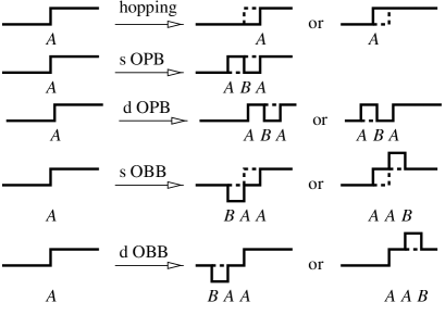
FIG. 1.: Step hopping and branching processes of an up step (an $A$ type particle). The letters $s$ and $d$ represent static and dynamic type branching, respectively. The dashed lines denote the surface before each event. Dynamic events near B particles are identical by mirror symmetry.

FIG. 2.: Phase diagram of our model. $\tilde{r}=r/p$ is the probability for OBB type branching (creating local surface roughness) and $\tilde{q}=q/p$ is the probability for OPB type branching (creating disordered flat type local order), relative to the hopping probability $p$. $y_{r}$ and $y_{T}\equiv 1/\nu_{\perp}$ are the scaling dimensions of the OBB and OPB operators, respectively.

FIG. 3.: Semi-log plots of the effective exponents $\eta$ and $\delta$ versus $1/t$ for several values of $\tilde{q}$ close to criticality. The data at our best estimate for the critical point $\tilde{q}_{c}$ are highlighted as thick lines.

FIG. 4.: (a) Decay of the step density at $\tilde{q}=\tilde{q}_{c}$. Each curve corresponds to $L=2^{5},\ldots,2^{10}$ from top to bottom. From the asymptotic slope of the curves we obtain $\beta/\nu_{\parallel}=0.282(5)$. The broken line is of slope 0.282. The inset shows the finite size scaling of the saturated step density. From the slope we obtain $\beta/\nu_{\perp}=0.497(5)$. The broken line has slope 0.497. (b) Scaling plot for $\log_{10}\left[\rho_{0}L^{\beta/\nu_{\perp}}\right]$ against $\log_{10}\left[\delta\tilde{q}L^{1/\nu_{\perp}}\right]$. Using the values of $\tilde{q}_{c}$ from defect dynamics simulations and $\beta/\nu_{\perp}$ in (a), the best data collapse is obtained with $\nu_{\perp}=1.78$.

FIG. 5.: The surface width in the rough phase at $\tilde{q}=\tilde{r}=1.0$. The curves correspond to system sizes $L=2^{5},\ldots,2^{9}$. The width obeys the scaling form $W=L^{2\alpha}f(t/L^{\alpha/\beta})$ with the Edwards-Wilkinson exponents $\alpha=1/2$, $\beta=1/4$, and $z=\alpha/\beta=2$ as shown in the inset.

FIG. 6.: Scaling of the spreading velocity $v$ of the active region. Different symbols are used for $v_{1}~{}(+)$, $v_{2}~{}(\times)$, $v_{3}~{}(\circ)$, $v_{4}~{}(\bigtriangleup)$, and $v_{\rm{eff.}}$ ($\Box$). The $v_{k\geq 3}$ merge into $v_{\rm{eff.}}$, which confirms that $v_{\rm{eff.}}$ is the asymptotic value for $v$.

FIG. 7.: Schematic typical surface configurations at the absorbing side of the DI transition, $0<\tilde{q}<\tilde{q}_{c}$.

FIG. 8.: Schematic surface configurations at $q=1$. They illustrate that hopping of the solitons requires a sequence of two branching processes.

FIG. 9.: The particle density $\rho$ vs. $t$ at point $S$. The dashed line has the expected slope $-1/4$. The inset shows that the effective exponent $\theta(t)$ approaches $1/4$ with a power law correction, i.e., $\theta(t)-1/4\sim t^{-1/8}$. The dashed line in the inset has the predicted slope $1/8$.

FIG. 10.: Estimates for the density exponents. The squares ($\Box$), up-triangles ($\bigtriangleup$), and down-triangles ($\bigtriangledown$) correspond to $k=1,2,$ and 3, respectively. The predicted values of the exponents are represented by solid lines and circles.

- [1] For a review see J. Marro and R. Dickman, Nonequilibrium Phase Transitions in Lattice Models (Cambridge University Press, Cambridge, 1996).
- [2] T. M. Liggett, Interacting Particle Systems (Springer-Verlag, New York, 1985).
- [3] P. Grassberger and A. de la Torre, Ann. Phys. (N.Y.) 122, 373 (1979).
- [4] I. Jensen, Phys. Rev. Lett. 70, 1465 (1993).
- [5] H. Takayasu and A. Yu. Tretyakov, Phys. Rev. Lett. 68, 3060 (1992).
- [6] P. Grassberger, F. Krause, and T. von der Twer, J. Phys. A 17 L105 (1984); P. Grassberger, J. Phys. A 22, L1103 (1989).
- [7] N. Menyh́ard, J. Phys. A 27, 6139 (1994); N. Menyh́ard and G. Ódor, J. Phys. A 28, 4505 (1995).
- [8] M. H. Kim and H. Park, Phys. Rev. Lett. 73, 2597 (1994); H. Park, M. H. Kim and, H. Park, Phys. Rev. E 52, 5664 (1995).
- [9] I. Jensen, Phys. Rev. E 50, 3623 (1994).
- [10] H. Park and H. Park, Physica A 221, 97 (1995).
- [11] H. Hinrichsen, Phys. Rev. E 55, 219 (1997).
- [12] W. Hwang, S. Kwon, H. Park and, H. Park, Phys. Rev. E 57, 6438 (1998).
- [13] W. Hwang and H. Park (unpublished).
- [14] J. D. Noh (unpublished).
- [15] J. L. Cardy and U. C. Täuber, Phys. Rev. Lett. 77, 4780 (1996).
- [16] S. F. Edwards and D. R. Wilkinson, Proc. R. Soc. Lond. A 381, 17 (1982).
- [17] K. Rommelse and M. den Nijs, Phys. Rev. Lett. 59, 2578 (1987).
- [18] M. den Nijs, chapter 4 in The Chemical Physics of Solid Surfaces and Heterogeneous Catalysis, vol. 7 edited by D. King, Elsevier (Amsterdam, 1994).
- [19] S. Kwon and H. Park, Phys. Rev. E 52, 5955 (1995).
- [20] A. Sudbury, Ann. Prob. 18, 581 (1990); H. Takayasu and N. Inui, J. Phys. A 25, L585 (1992).
- [21] A smooth (but not perfectly flat) phase was found stable against the roughening degree of freedom in other models [30]. But this is not a true absorbing phase where the dynamics are completely dead.
- [22] The critical point of the BAW model with dynamic branching is at [19]. In our model, some branching processes are rejected as explained in section 3. So the absorbing phase in our model becomes a little bit larger than in the BAW model.
- [23] J. F. F. Mendes, R. Dickman, M. Henkel, and M. C. Marques, J. Phys. A 27, 3019 (1994).
- [24] This is the conventional definition of the dynamic exponent . We do not take the traditional usage of as the exponent of the mean-square distance of spreading at the absorbing transition. This spreading exponent can be expressed as in terms of the dynamic exponent .
- [25] M. Bramson and J. L. Lebowitz, Phys. Rev. Lett. 61, 2397 (1988); J. Stat. Phys. 62, 297 (1991).
- [26] D. Toussaint and F. Wilczek, J. Chem. Phys. 78, 2642 (1983).
- [27] K. Kang and S. Redner, Phys. Rev. Lett. 52, 955 (1984).
- [28] F. Leyvraz and S. Redner, Phys. Rev. A 46, 3132 (1992).
- [29] The distances between nearest neighbour clouds of the same species () and opposite species () diverge with different exponents. The divergence of the cloud widths is limited by these distances, and therefore depends on their local neighbourhoods. It suffices to deal with the average distance , as done in the text, since is the slowest of the two and turns out to dominate.
- [30] U. Alon, M. R. Evans, H. Hinrichsen, and D. Mukamel, Phys. Rev. Lett. 76, 2746 (1996); Phys. Rev. E 57, 4997 (1998).
- [31] M. Kardar, G. Parisi, and Y. C. Zhang, Phys. Rev. Lett. 56, 889 (1986).