Faceting Transition in an Exactly Solvable Terrace-Ledge-Kink Model

Abstract

We solve exactly a Terrace-Ledge-Kink (TLK) model describing a crystal surface at a microscopic level. We show that there is a faceting transition driven either by temperature or by the chemical potential that controls the slope of the surface. In the rough phase we investigate thermal fluctuations of the surface using Conformal Field Theory.

I Introduction

In this paper, we reexamine a model of crystal surfaces in three dimensions [2], which is inspired by the Terrace-Ledge-Kink (TLK) [3] ideas of Kossel and Stransky [4]. By careful specification, an isomorphism can be established between our system and an extension of the six-vertex models [5], which allows an exact discussion at a thermodynamic level of the different types of phase transitions which take place. We complement this with recent relevant deductions from conformal field theory, which give microscopic insight. We shall return to this six-vertex isomorphism after the next few paragraphs, in which we describe the model and outline the results.

Consider a vicinal section of a crystal surface, that is one which on average is tilted by a small angle from a closed packed plane. Let this underlying plane have normal $(001)$ and let the normal to the mean vicinal surface lie in the plane containing $(001)$ and $(101)$. Following Kossel and Stransky [4], we give the vicinal surface a microscopic structure by regarding it as the upper surface of a set of unit cubes, each of which representing a molecule or atom, which are stacked vertically with no voids, thereby covering the basal plane $(x,y,0)$ with columns of cubes. We shall make a somewhat eccentric choice of lattice structure, which is described in detail below, and which will turn out to be of crucial importance in the statistical-mechanical modelling of the short-ranged interactions between ledges.

We now impose the vicinal condition by making the height on the left extremum of the surface equal to zero, and the height on the right one equal to some constant positive integer. These extrema intersect the lines $(0,y)$ and $(M,y)$ of $\Lambda$ as zig-zags or zippers, as shown in Fig. 4. Connected components of the upper surface having the same height are termed terraces and are separated from other terraces by ledges, which can have bends through an angle of $\pi/2$: these are termed kinks.

In this paper, we shall make two further restrictions: firstly, there are no adatoms or pits on the terraces; and secondly, ledges cannot separate adjacent terraces with a height difference greater than unity. This means that different ledges can never coincide and that no ledge can form a closed loop: each ledge begins at the bottom of the lattice and exits at the top.

We emphasize that the above construction is not the only way of generating exactly solvable models. Other routes are the BCSOS [6, 7] and the surface deconstruction [8] model. There is also the Hamiltonian limit type of approximation proposed by Jayaprakash et al. [9] and by Burkhardt and Schlottmann [10], together with other work by Villain et al. [11] and by Bartelt et al. [12]. There is a general review of morphology of vicinal surfaces in [13]. For small tilt angles $\theta$, a polynomial approximation is given to the surface free energy $f(\theta)$ where

$$f(\theta)=f(0)+a\theta+b\theta^{3}$$ (1)

in which $a$ is related to the kink energy and $b$ comes from ledge-ledge interactions which can be entropic in character, elastic (although the distinction between these two is not entirely clear) or coming from electrostatic dipolar interactions in metals. We scrutinize (1) from our exact solution and also analyse the ledge-ledge interaction from first principles in appendix E.

Our model shows the formation of a crystal facet at half-filling, which we can regard as at a tilt angle of $\pi/4$. In the low-temperature phase, the surface height fluctuations about the $\pi/4$ tilted plane are of order one, but above the faceting temperature there is power-law decay of ledge-ledge correlation functions, making Kosterlitz-Thouless [16] behaviour extremely likely. As we shall see, for a certain nonzero repulsion between ledges we get a free-fermionic structure of the transfer matrix, and in this case the height fluctuations are shown to be of Kosterlitz-Thouless type.

Finally, we note that our model is closely related to a lattice regularization of the anisotropic principal chiral field [14].

II The model

We consider a square lattice tilted by 45 degrees (see Fig. 1 (a)), and define a configuration by declaring each link between two lattice sites to be occupied (state up, denoted 1) or empty (state down, denoted 2). We then impose the six-vertex constraint or ice rule: at each vertex (centered at lattice sites) the number of occupied links must be conserved between top and bottom. An example of an allowed configuration is shown in Fig. 1(a), where the occupied links are drawn as thick lines.

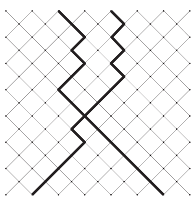
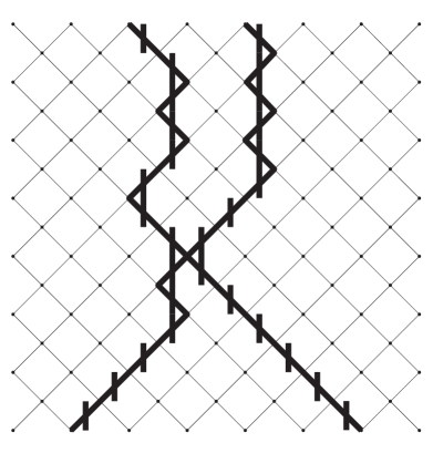
FIG. 1.: (a) six-vertex model configuration; (b) definition of ledge segments for a given six-vertex configuration.

Every such allowed configuration can now be mapped onto a configuration of terraces, ledges and kinks defining a surface. We first introduce ledges by drawing short vertical lines through the middle of each occupied link (see Fig. 1(b)). These segments are then connected by horizontal lines representing kinks, as shown in Fig. 2(a). Treating ledges and kinks as steps on a surface, the above procedure then defines terraces, which are indicated by different shades of grey in Fig. 2(b). Figure  4 explicits the three-dimensional structure.

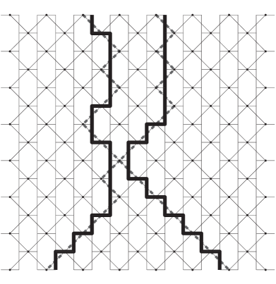
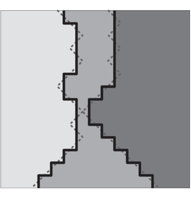
FIG. 2.: Square lattice configurations in the TLK model: (a) ledges and kinks; (b) terraces.

The above procedure leads to a number of restrictions on the allowed configurations of terraces, ledges and kinks. For example ledges cannot form closed loops, and there cannot be multiple kinks.

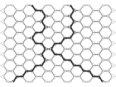
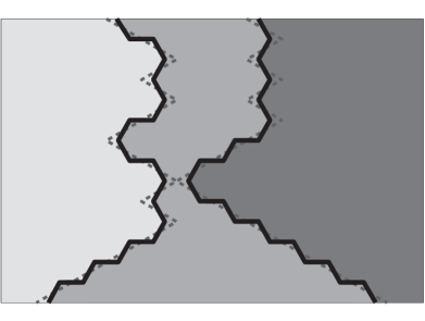
FIG. 3.: A configuration in the TLK model with the hexagonal lattice.

This last restriction can be effectively removed by a slight modification of the ledge representation. Stretching the lattice by $\sqrt{3}$ in the horizontal direction we can introduce a lattice of regular hexagons, and use the sides of these hexagons to define the ledges and kinks as shown in Fig. 3. In this case the restrictions on multiple kinks are built into the lattice structure.

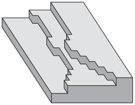
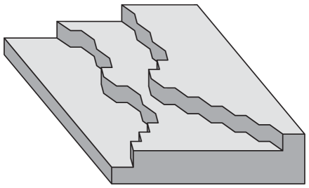
FIG. 4.: Section of a crystal surface: (a) square lattice; (b) hexagonal lattice.

We therefore end up with two slightly different geometrical representations for the configurations: in Fig. 4 (a) the underlying lattice is square, although there are restrictions in the allowed configurations which involve the tiling of Fig. 2; in Fig. 4 (b) the terrace-ledge-kink structure is placed on a hexagonal lattice.

We now associate a weight with each configuration.

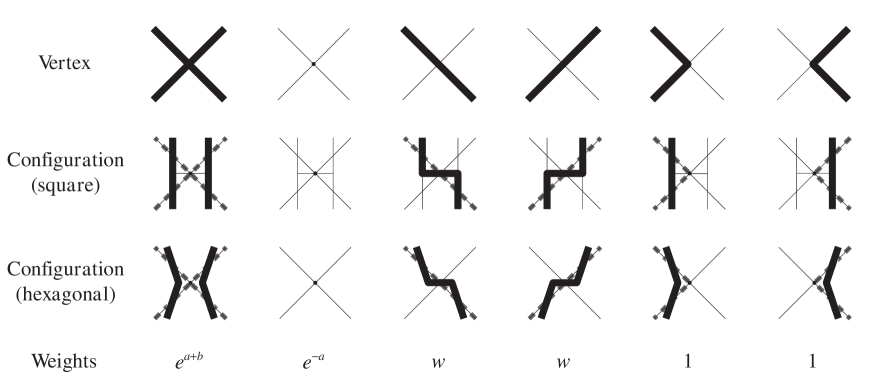
FIG. 5.: Six-vertex vertices and the two possible interpretations in terms of ledges.

In terms of the underlying six-vertex model we associate a Boltzmann weight according to the rule shown in Fig. 5 with each vertex. The weight $w$ is a kink fugacity, and lower values of $w$ correspond to stiffer ledges. The weights also depend on the interaction energy $b$ between neighbouring ledges and the ledge stiffness (note that in our model only neighbouring ledges interact and that by construction ledges can never cross each other). The parameter $a$ is a ledge fugacity or chemical potential, which controls the number of ledges, or equivalently the slope of the crystal surface.

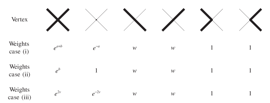
FIG. 6.: The three different assignments of vertex weights discussed in the text.

We now discuss the relationships between the three weight assignments shown on Fig. 6. Some aspects of the Bethe Ansatz for (ii) have been discussed in [2]. The Bethe Ansatz generates eigenvectors for the $(1,1)$ transfer matrix with fixed fraction of up arrows, corresponding to a given vicinal section angle. The solution gives the limiting free energy per unit area, in principle for all angles, but in closed form by Fourier methods only for the half-filled case. It was argued that there are two quite distinct types of phase transition, which occur at the solutions of $e^{b}=(1\pm w)^{2}$.

For $b>0$ (attraction between ledges), there is a reconstructive phase transition at a temperature $T(b)$ to a state with zero limiting entropy for $T<T(b)$. As the temperature approaches $T(b)$ from above, the specific heat diverges as $(T-T(b))^{-1/2}$ (cf. end of appendix E; this is similar to [15]).

In this paper, we focus on the transition at $e^{b}=(1-w)^{2}$, for $b<0$, implying repulsion between the ledges. This problem was discussed in the fixed vertical polarization case with the $(1,1)$ transfer matrix in [2]. There it was found that at half-filling the system displays an infinite-order phase transition similar to the Kosterlitz-Thouless one [16], or the van Beijeren one in the BCSOS case [6].

We consider the weight assignment (i) of Fig. 6 and we use a Legendre transform with respect to the variable $a$, with no fixing of the polarization, in order to go to the physical situation of case (ii) with fixed polarization. Notice that neither (i) nor (ii) is equivalent to the usual $(h,v)$ field scenario in the six-vertex model (iii): new results are needed. We note that the model (i) is not the same as (ii) because the chemical potential $a$ is not always an invertible function of the ledge number. In other words, the model [2] contains phases that are not accessible by tuning $a$ in the model considered here. The situation is analogous to the six-vertex model in a vertical field or equivalently the Heisenberg XXZ chain in a magnetic field $H$. If we consider the ferromagnet in the sector with fixed magnetization the ground state is rather complicated [17]. This phase is not accessible by tuning the magnetic field and considering the absolute ground state (i.e. the minimal energy state in the grand canonical ensemble where the number of up/down spins is variable) as the ground state will always be the saturated ferromagnetic state with all spins up or down.

We use the Quantum Inverse Scattering Method, which is reviewed in [18], to derive new results, as well as the old ones in a formulation which may be more familiar for most readers. We calculate:

$$E(a,b)=\lim_{\Lambda\to\infty}\frac{1}{|\Lambda|}\log Z_{\Lambda}(a;b,w)$$ (2)

where

$$Z_{\Lambda}(a;b,w)={\rm Trace}\prod_{j=1}^{|\Lambda|}e^{bn_{1}}e^{a(n_{1}-n_{2})}w^{n_{3}+n_{4}}$$ (3)

where the trace is taken over all ice-rule-compliant configurations on $|\Lambda|=MN$ points for a $M\times N$ lattice; $n_{j}$ is the number of vertices of type $j=1,2,\dots,6$ in the lattice configuration. The free energy for fixed polarization is then given by

$$F(m;b,w)=\sup_{a}(E(a,b)-ma).$$ (4)

Correlation functions may be calculated in either ensemble by appropriately relating $m$ and the optimal $a={\hat{a}}(m)$ in (4), which is unique provided that $\partial E/\partial a$ exists at $a={\hat{a}}(m)$.

The paper is structured as follows. In section III, we give the Bethe Ansatz equations and expressions for the eigenvalues of the transfer matrix. A detailed derivation of these results, as well as the classification of the model in the framework of the Quantum Inverse Scattering Method, appears in appendix A. In section IV we discuss the phase diagram and calculate explicitly the free energy. In section V we give a precise definition of height and height-difference correlation functions. Sections VI and VII are concerned with the determination of the large-distance behaviour of these correlation functions. Finally we summarize our results and discuss their relevance in relation to other theoretical and experimental work.

There are several further appendices discussing some technical aspects of our work: the free-fermion case is solved explicitly in appendix B, and appendix C deals with the analysis of the Bethe Ansatz equation in the case of negative kink energy, where novel peculiarities concerning the distribution of roots in the complex plane are encountered. Appendix D gives the second-quantized form of the transfer operator, and in appendix E we discuss effective interactions between ledges and some low-angle expansions.

III Bethe Ansatz equations

Denoting the weight matrix by $R$ we have in case (i):

$$R^{11}_{11}=e^{a+b}\ ,\qquad R^{22}_{22}=e^{-a}\ ,\qquad R^{12}_{21}=w\ ,\qquad R^{21}_{12}=w\ ,\qquad R^{12}_{12}=1\ ,\qquad R^{21}_{21}=1\ .$$ (5)

The vertex model defined by (5) is exactly solvable by Bethe Ansatz. In [2] a particular parametrization of the Bethe Ansatz equations (for the case $a=0$) was derived using coordinate space techniques. In appendix A we show that the model (5) can actually be embedded into a family of commuting transfer matrices and derive a parametrization of the Bethe Ansatz equations in terms of entire functions. In the language of the Quantum Inverse Scattering Method [18] the model (5) is simply a particular case of an inhomogeneous asymmetric 6-vertex model [19, 5, 20]. As is shown in appendix A, it is convenient to introduce parameters $\gamma$, $\omega$ and $v$ such that

$$e^{b}=\frac{\sin^{2}(\gamma-\omega/2)}{\sin^{2}\gamma},\qquad w=-\frac{\sin\omega/2}{\sin\gamma},\qquad e^{-a}=e^{-2v}\frac{\sin(\gamma-\omega/2)}{\sin\gamma}.$$ (6)

Eigenstates of the transfer matrix (with $2N-M$ ledges) are parametrized in terms of rapidity variables $\lambda_{k}$, which are subject to the following set of coupled algebraic equations, called Bethe Ansatz equations

$$\left(\frac{\sinh\left(\lambda_{k}+i\frac{\gamma}{2}\right)}{\sinh\left(\lambda_{k}-i\frac{\gamma}{2}\right)}\ \frac{\sinh\left(\lambda_{k}-i\frac{\omega-\gamma}{2}\right)}{\sinh\left(\lambda_{k}-i\frac{\omega+\gamma}{2}\right)}\right)^{N}=-\prod_{j=1}^{M}\frac{\sinh\left(\lambda_{k}-\lambda_{j}+i{\gamma}\right)}{\sinh\left(\lambda_{k}-\lambda_{j}-i{\gamma}\right)}\ ,\ k=1\ldots M\ .$$ (7)

The eigenvalues of the operator of translation by two sites are given by

$$\exp\left(iP(\{\lambda_{j}\})\right)=\prod_{k=1}\frac{\sinh\left(\lambda_{k}-i\frac{\gamma}{2}\right)}{\sinh\left(\lambda_{k}+i\frac{\gamma}{2}\right)}\ \frac{\sinh\left(\lambda_{k}-i\frac{\omega+\gamma}{2}\right)}{\sinh\left(\lambda_{k}-i\frac{\omega-\gamma}{2}\right)}\ ,$$ (8)

and the eigenvalues $\Lambda_{dd}$ of the diagonal-to-diagonal transfer matrix $\tau_{dd}$ are

$$\Lambda_{dd}(\{\lambda_{j}\})=e^{2a(M-N)}\left(\frac{\sin(\gamma-\frac{\omega}{2})}{\sin\gamma}\right)^{2M}\prod_{j=1}^{M}\frac{\sinh\left(\lambda_{j}+i\frac{\gamma}{2}\right)}{\sinh\left(\lambda_{j}-i\frac{\gamma}{2}\right)}\frac{\sinh\left(\lambda_{j}-i\frac{\gamma+\omega}{2}\right)}{\sinh\left(\lambda_{j}+i\frac{\gamma-\omega}{2}\right)}\ .$$ (9)

IV Phase diagram

The parametrization (6) is such that $\gamma$ and $\omega$ cannot always chosen to be real. Furthermore, due to the fact that $a$ and $b$ must be real and $w$ must be real and between $0$ and $1$ there are restrictions on the regions of “physical” $\gamma$ and $\omega$. As $a$ and $b$ are real so is $v$, and by exchanging up and down spins in the Bethe Ansatz solution (see appendix A) we can restrict ourselves to the case $v<0$.

The permitted values of $b$ and $w$ are covered by the following three regimes of $\gamma$ and $\omega$:

• Region (1a): $\gamma$ and $\omega$ are real with $0<\gamma<\pi/2$ and $-2\gamma<\omega<0$;

• Region (1b): $\gamma$ and $\omega$ are real with $\pi/2<\gamma<\pi$ and $-2\pi+2\gamma<\omega<0$;

• Region (2): $\gamma$ and $\omega$ are purely imaginary. It is convenient to choose a parametrization obtained from (6) and (7) by taking $\gamma\to i\gamma$, $\omega\to i\omega$ and $\lambda\to i(\lambda+\pi/2)$, which leads to the following set of equations

  $$e^{b}=\frac{\sinh^{2}(\gamma-\omega/2)}{\sinh^{2}\gamma},\qquad w=-\frac{\sinh\omega/2}{\sinh\gamma},\qquad e^{-a}=e^{-2v}\frac{\sinh(\gamma-\omega/2)}{\sinh\gamma},$$ (10)

  where $\gamma>0$ and $-2\gamma<\omega<0$,

  $$\left(\frac{\cos\left(\lambda_{k}+i\frac{\gamma}{2}\right)}{\cos\left(\lambda_{k}-i\frac{\gamma}{2}\right)}\ \frac{\cos\left(\lambda_{k}-i\frac{\omega-\gamma}{2}\right)}{\cos\left(\lambda_{k}-i\frac{\omega+\gamma}{2}\right)}\right)^{N}=-\prod_{j=1}^{M}\frac{\sin\left(\lambda_{k}-\lambda_{j}+i{\gamma}\right)}{\sin\left(\lambda_{k}-\lambda_{j}-i{\gamma}\right)}\ ,\ k=1\ldots M\ .$$ (11)

  $$\Lambda_{dd}(\{\lambda_{j}\})=e^{2a(M-N)}\left(\frac{\sinh(\gamma-\frac{\omega}{2})}{\sinh\gamma}\right)^{2M}\prod_{j=1}^{M}\frac{\cos\left(\lambda_{j}+i\frac{\gamma}{2}\right)}{\cos\left(\lambda_{j}-i\frac{\gamma}{2}\right)}\frac{\cos\left(\lambda_{j}-i\frac{\gamma+\omega}{2}\right)}{\cos\left(\lambda_{j}+i\frac{\gamma-\omega}{2}\right)}\ .$$ (12)

• Region (3): $\omega$ and $\gamma-\pi$ are purely imaginary. A convenient parametrization is then

  $$e^{b}=\frac{\sinh^{2}(\gamma-\omega/2)}{\sinh^{2}\gamma},\qquad w=\frac{\sinh\omega/2}{\sinh\gamma},\qquad e^{-a}=e^{-2v}\frac{\sinh(\gamma-\omega/2)}{\sinh\gamma},$$ (13)

  where $2\gamma>\omega>0$. We substitute $\lambda\to i(\lambda+\pi/2)$. The Bethe Ansatz equations become

  $$\left(\frac{\sin\left(\lambda_{k}+i\frac{\gamma}{2}\right)}{\sin\left(\lambda_{k}-i\frac{\gamma}{2}\right)}\ \frac{\sin\left(\lambda_{k}-i\frac{\omega-\gamma}{2}\right)}{\sin\left(\lambda_{k}-i\frac{\omega+\gamma}{2}\right)}\right)^{N}=-\prod_{j=1}^{M}\frac{\sin\left(\lambda_{k}-\lambda_{j}+i{\gamma}\right)}{\sin\left(\lambda_{k}-\lambda_{j}-i{\gamma}\right)}\ ,\ k=1\ldots M\ .$$ (14)

  The eigenvalues of $\tau_{dd}$ are

  $$\Lambda_{dd}(\{\lambda_{j}\})=e^{2a(M-N)}\left(\frac{\sinh(\gamma-\frac{\omega}{2})}{\sinh\gamma}\right)^{2M}\prod_{j=1}^{M}\frac{\sin\left(\lambda_{j}+i\frac{\gamma}{2}\right)}{\sin\left(\lambda_{j}-i\frac{\gamma}{2}\right)}\frac{\sin\left(\lambda_{j}-i\frac{\gamma+\omega}{2}\right)}{\sin\left(\lambda_{j}+i\frac{\gamma-\omega}{2}\right)}\ .$$ (15)

By analysing the Bethe Ansatz equations in the various regions we can determine the largest eigenvalues of the transfer matrix and thus establish the phase diagram of the model.

A Phase diagram for $v=0$

As in the case of the symmetric six-vertex model the phase structure of the TLK model for vanishing vertical field $v=0$ is closely related to the parametrization of the Bethe Ansatz equations. We find that there are three different phases corresponding to the three different regimes in $\gamma$ and $\omega$ discussed above. Phase 1 is a critical (rough) phase whereas Phase 2 and Phase 3 correspond to massive phases (smooth surfaces). They are the analogs of the ferro (2) and antiferroelectric (3) phases in the symmetric six-vertex model. The resulting phase diagram for $v=0$ is shown in Fig. 7.

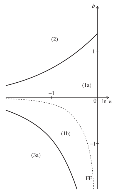
FIG. 7.: Phase diagram for zero vertical field $v=0$.

The precise parametrization of the phase boundaries for $v=0$ is as follows: the boundary between Region (1) and Region (2) corresponds to $\gamma$ and $\omega$ small with $\omega/\gamma$ finite, and

$$e^{b}=(1+w)^{2}\qquad{\rm with}\qquad w=-\frac{\omega}{2\gamma}\ .$$ (16)

The boundary between Region (1) and Region (3) is for $\gamma-\pi$ and $\omega$ small with $\omega/(\pi-\gamma)$ finite

$$e^{b}=(1-w)^{2}\qquad{\rm with}\qquad w=-\frac{\omega}{2(\pi-\gamma)}\ .$$ (17)

B Phase diagram for $v<0$

We now discuss the phase diagram as a function of $v$ for various points in the $(\gamma,\omega)$ plane. The situation is analogous to the one for the XXZ Heisenberg chain in a magnetic field [21]. As far as the parametrization of the Bethe Ansatz equations is concerned, the $(\gamma,\omega)$ plane is divided into Regions (1)-(3) as discussed above. At $v=0$ the phase structure of the model exactly reflects this division of the $(\gamma,\omega)$ plane.

• Let us consider a fixed point $P_{1}=(\gamma_{1},\omega_{1})$ in Region (1). At $v=0$ the model is thus critical. As $v$ is decreased the phase boundary between Phase 1 and Phase 2 moves in negative $b$ direction and eventually encompasses $P_{1}$: the model is then massive and we are in the ferroelectric phase. $P_{1}$ remains in Phase 2 as $v$ is decreased further.

• Next we consider a point $P_{2}=(\gamma_{2},\omega_{2})$ in Region (2). For any value of $v\leq 0$ the model is in Phase 2.

• Finally we consider a point $P_{3}=(\gamma_{3},\omega_{3})$ in Region (3). At $v=0$ the model is in the massive Phase 3. As $v$ decreases the phase boundary between Phase 1 and Phase 3 is shifted in the negative $b$ direction and eventually $P_{3}$ enters Phase 1. As $v$ is decreased further, $P_{3}$ finally enters into Phase 2.

The above picture, together with the precise parametrization of the phase boundaries for $v<0$, follows from the analysis of the largest eigenvalues of $\tau_{dd}$, which is outlined in the next subsection. The change of the phase boundaries under a decrease of $v$ is shown in Fig. 8. The corresponding ledge chemical potential tends to decrease the number of ledges in the system and as a result the transition to the state with no ledges (Phase 2) occurs at a smaller value of ledge attraction $b$ for fixed $w$. On the other hand the critical regime extends to stronger ledge repulsion.

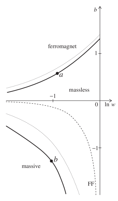
FIG. 8.: Phase diagram for $v=-0.025$ (solid lines) vs $v=0$ (dotted lines).

C Characterization of the Maximal Eigenvalue

Let us now turn to the distribution of rapidities $\lambda$ corresponding to the largest eigenvalue of $\tau_{dd}$ in the three phases. It is convenient to define an “energy” $E$ by

$$E(\{\lambda_{k}\})=-\ln|\Lambda_{dd}(\{\lambda_{k}\})|=2Na+\sum_{k=1}^{M}\epsilon_{0}(\lambda_{k})\ ,$$ (18)

where the “bare energy” of a single ledge $\epsilon_{0}(\lambda_{k})$ is given explicitly below. The maximal eigenvalue of $\tau_{dd}$ then corresponds to the minimal energy $E$. In the following we call the state corresponding to the largest eigenvalue of $\tau_{dd}$ the “ground state” of the system.

• Region (1): Let us start with the parametrization for the Bethe Ansatz equations and eigenvalues of the transfer matrix of Region (1). The contribution of a single ledge to the energy and to the eigenvalue of the 2-site translation operator (8) are

  $$\epsilon_{0}(\lambda) = -\log\left|\frac{\sinh\left(\lambda+i\frac{\gamma}{2}\right)\sinh\left(\lambda-i\frac{\gamma+\omega}{2}\right)}{\sinh\left(\lambda-i\frac{\gamma}{2}\right)\sinh\left(\lambda+i\frac{\gamma-\omega}{2}\right)}\right|-4v\ ,$$ (19)

  $$e^{ip_{0}(\lambda)} = \frac{\sinh(\lambda+i\gamma/2)\sinh(\lambda-i\omega/2+i\gamma/2)}{\sinh(\lambda-i\gamma/2)\sinh(\lambda-i\omega/2-i\gamma/2)}\ .$$ (20)

  In the following we restrict ourselves to solutions of the Bethe Ansatz equations for which

  $$\left|e^{ip_{0}(\lambda_{k})}\right|=1,\ k=1\ldots M.$$ (21)

  This means that we do not consider so-called string solutions [22, 19, 23] as they are not important for our present purposes: the largest few eigenvalues of $\tau_{dd}$ are given by solutions of (7) that fulfill (21).

  Rapidities fulfilling (21) are distributed on the two lines $\lambda=x+i\pi/2+i\omega/4$ and $\lambda=x+i\omega/4$. We find that $\epsilon_{0}(x+i\pi/2+i\omega/4)<0$ and $\epsilon_{0}(x+i\omega/4)>0$ for any real $x$. Therefore for $v<0$ the distribution of rapidities in the ground state is obtained by filling a Fermi sea of rapidities on the line $\lambda=x+i\pi/2+i\omega/4$ with $|x|\leq x_{F}$.

  The Fermi sea disappears if $\epsilon_{0}(i\omega/4)>0$ and the maximum eigenvalue state then contains no ledges at all. Thus for sufficiently large negative $v$ we are in the ferroelectric Phase 2. We exclude this case from the following discussion.

  In the thermodynamic limit the ground state is described by a continuous rapidity distribution function $\rho(x)$, which is defined by

  $$\rho(x_{k})=\lim_{N\to\infty}1/(N(x_{k+1}-x_{k}))\ ,$$ (22)

  where $\lambda_{k}=x_{k}+i\pi/2+i\omega/4$ are solutions of (7). The Bethe Ansatz equations turn into an integral equation for $\rho(x)$ in the thermodynamic limit, which is easily obtained by subtracting the logarithm of (7) for $k$ and $k+1$ and then turning sums into integrals

  $$\rho(x)-\frac{1}{2\pi}\int_{-x_{F}}^{x_{F}}dy\ K(x-y)\rho(y)=\rho_{0}(x),$$ (23)

  where

  $$K(x) = -\frac{2\sin 2\gamma}{\cosh 2x-\cos 2\gamma}\ ,$$ (24)

  $$\rho_{0}(x) = \frac{1}{2\pi}\frac{dp_{0}}{dx}=\frac{1}{\pi}\left(\frac{\sin(\gamma+\omega/2)}{\cosh 2x+\cos(\gamma+\omega/2)}+\frac{\sin(\gamma-\omega/2)}{\cosh 2x+\cos(\gamma-\omega/2)}\right).$$ (25)

  The ground state energy density is then given by

  $$E_{GS}=\int_{-x_{F}}^{x_{F}}dy\ \rho(y)\ \epsilon_{0}(y+i\pi/2+i\omega/4)\ ,$$ (26)

  where $x_{F}$ is determined self-consistently by the condition

  $$\frac{\delta E_{GS}}{\delta x_{F}}\bigg{|}_{v}=0.$$ (27)

  The density of ledges in the ground state as a function of $v$ is then given by

  $$D=\int_{-x_{F}}^{x_{F}}dx\ \rho(x)\ .$$ (28)

  Note that $D=1$ corresponds to one ledge per two sites, i.e. half-filling because there are $2N$ sites in $x$-direction. In the square lattice representation, if we assume that the step height corresponding to a ledge is equal to two lattice steps, then the tilt angle of the surface with ledge density $D$ is given by $\tan\theta=D$. The angle corresponding to half filling is then $\theta=\pi/4$, and we denote by $\theta_{f}=\arctan(2)$ the angle for full filling.

  It is easier to work with the so-called dressed energy $\epsilon(x)$ defined by

  $$\epsilon(x)-\frac{1}{2\pi}\int_{-x_{F}}^{x_{F}}dy\ K(x-y)\ \epsilon(y)=\epsilon_{0}(x+i\pi/2+i\omega/4),$$ (29)

  where we demand that $\epsilon(x_{F})=0$. This fixes $x_{F}$ as a function of $v$ and it can be shown that

  $$E_{GS}=\int_{-x_{F}}^{x_{F}}dy\ \rho_{0}(y)\ \epsilon(y)\ .$$ (30)

  In order to calculate the ground state energy one now simply solves (29) and (30) numerically (analytic solutions are not possible for generic $v<0$). As remarked above we are dealing with a critical phase. In order to facilitate the calculation of correlation functions we need to determine the finite-size correction to the ground state energy, which is related [24] to the central charge of the underlying conformal field theory [25]. The leading corrections are determined by using the Euler-Maclaurin sum formula when turning sums into integrals [26, 18]. We find

  $$E_{GS}(N)=\int_{-x_{F}}^{x_{F}}dy\ \epsilon_{0}(y+i\pi/2+i\omega/4)\ \rho(y)-\frac{\pi}{6N}\frac{\epsilon^{\prime}(x_{F})}{2\pi\rho(x_{F})}.$$ (31)

  This can be expressed in terms of the Fermi velocity

  $$v_{F}=\frac{\partial\epsilon(x)/\partial x}{\partial p(x)/\partial x}\biggr{|}_{x=x_{F}}=\frac{\epsilon^{\prime}(x_{F})}{2\pi\rho(x_{F})}\ ,$$ (32)

  where $p(x)$ is the dressed momentum

  $$p(x)=\int_{-x_{F}}^{x_{F}}dx\ \rho(x)\ p_{0}(x)\ .$$ (33)

  As a result we have that the central charge of the critical theory is, as expected, $c=1$.

• Region (2): For any $v<0$, we have that $\epsilon_{0}(x+i\pi/2+i\omega/4)>0$ and $\epsilon_{0}(x+i\omega/4)>0$. As strings do not play a role, the ground state is the one with no ledges.

• Region (3): In this region we need to analyse the Bethe Ansatz equations (14). As we already mentioned we encounter three different phases by varying $v$. For $v$ close to zero the ground state is obtained by filling a Fermi sea of rapidities $\lambda=x+i\omega/4$ with $x\in[-\pi/2,\pi/2]$. The ground state energy is given by (30) with $x_{F}=\pi/2$, where the dressed energy $\epsilon(x)$ fulfills

  $$\epsilon(x)+\frac{1}{2\pi}\int_{-x_{F}}^{x_{F}}dy\ \frac{2\sinh(2\gamma)}{\cosh(2\gamma)-\cos(2x-2y)}\ \epsilon(y)=\epsilon_{0}(x)\ ,$$ (34)

  but does not vanish at the Fermi rapidity $\pi/2$, i.e. $\epsilon(\pm\pi/2)<0$. The bare energy and momentum that enter (30) and (34) are given by

  $$\epsilon_{0}(x) = -\log\left|\frac{\cosh(\gamma+\omega/2)-\cos(2x)}{\cosh(\gamma-\omega/2)-\cos(2x)}\right|-4v\ ,$$ (35)

  $$\rho_{0}(x) = -\frac{1}{2\pi}\frac{dp_{0}}{dx}=\frac{1}{\pi}\left(\frac{\sinh(\gamma+\omega/2)}{\cosh(\gamma+\omega/2)-\cos 2x}+\frac{\sinh(\gamma-\omega/2)}{\cosh(\gamma-\omega/2)-\cos 2x}\right).$$ (36)

  As $v$ increases in magnitude $x_{F}$ stays at $\pi/2$ until, for $|v|$ larger than some critical value $v_{c}$, it starts to decrease. The critical value is characterized by

  $$\epsilon(\pi/2)\bigg{|}_{v=v_{c}}=0\ .$$ (37)

  For values of $|v|$ slightly larger than $v_{c}$ we are in Phase 1. Energy and ledge density are obtained from the same integral equations as before, but now $x_{F}<\pi/2$. Finally, as $|v|$ continues to increase it reaches a second critical value $v_{c}^{\prime}$ at which a transition to the ferroelectric Phase 2 occurs and the ground state becomes trivial.

In Fig. 9 we plot the ledge density as a function $v$ for two points in the $(\gamma,\omega)$ plane. These points, denoted by $a$ and $b$, are chosen such that they lie on phase boundaries for $v=-0.025$ (see Fig.  8). For $v=0$ point $a$ is within the Phase 1 and the ledge density is 1. As $|v|$ decreases to $v=-0.025$ the ledge density decreases until it becomes zero: there is a transition to Phase 2. For $v<-0.025$ we remain in Phase 2 and accordingly $D=0$. Point $b$ is in the massive Phase 3 for $v=0$ and as $v$ decreases from $0$ the ledge density remains $1$ until at $v_{c}=-0.025$ we enter the Phase 1 and $D$ starts to decrease until it reaches zero at $v_{c}^{\prime}=-0.38$. For $v<v_{c}^{\prime}$ point $b$ belongs to Phase 2.

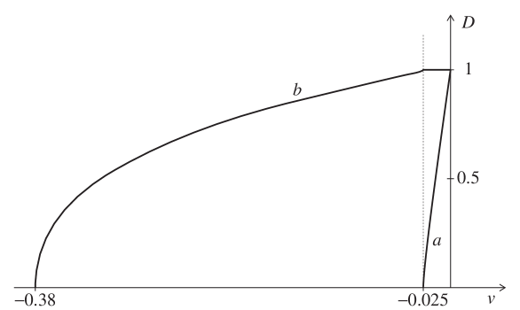
FIG. 9.: Density as a function of the ledge chemical potential $v$ for two points in the ($\gamma,\omega$)-plane.

V Height correlation functions

We now define a function $h(x,y)$, which measures the height of the surface at position $(x,y)$, where the coordinate system is such that the transfer direction is parallel to the $y$ axis. Due to the lattice structure, $h$ is constant on rectangles of size $(1,2)$ centred on points $(x+1/2,y-1/2)$, where $x$ and $y$ are integers with the same parity (see Fig. 10). It is thus sufficient (and indeed most convenient) to measure heights between such points only.

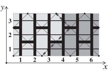
FIG. 10.: Local TLK configuration (for the square geometry).

Given the way that we defined the geometry of the surface in terms of ledges and kinks, which are directly related to the vertex model, it is clear that height correlation functions are nonlocal quantities. We therefore consider height-differences. For any point $(x,y)$ where the two coordinates have the same parity, the occupancy of the link centred on point $(x,y)$ is related to the height difference $d_{-}(x,y)=h(x+1/2,y-1/2)-h(x-1/2,y+1/2)$. This implies that $d_{-}(x,y)=0$ if the link is empty and $d_{-}(x,y)=+1$ if it is occupied. If $x$ and $y$ have different parities then we define $d_{+}(x,y)=h(x+1/2,y+1/2)-h(x-1/2,y-1/2)$. Here also $d_{+}(x,y)=+1$ if the link at $(x,y)$ is occupied and $d_{+}(x,y)=0$ otherwise.

The knowledge of the functions $d_{\pm}$ is sufficient to construct the height function $h$ up to an overall additive constant.

Since we impose periodic boundary conditions (in height differences), the expectation values of $d_{+}$ and $d_{-}$ are independent of the position. Moreover, because of invariance under the exchange of left and right, we have $\langle d_{+}\rangle=\langle d_{-}\rangle=D/2$, where $D$ is the ledge density $D=M/N$ (the system size of the system is taken to be $2N\times 2L$).

The correlation function $\langle d_{\alpha_{1}}(x_{1},y_{1})d_{\alpha_{0}}(x_{0},y_{0})\rangle$, where $\alpha_{i}=(-1)^{1+x_{i}+y_{i}}$ for $i=0,1$, depends only on $x_{1}-x_{0}$ and $y_{1}-y_{0}$ because of two-step translational invariance and left-right and up-down symmetries. Any height-difference correlation function of the model can therefore be obtained from the following connected correlation function, which is defined for all integer values of $x_{1}-x_{0}$ and $y_{1}-y_{0}$:

$$C^{c}(x_{1}-x_{0},y_{1}-y_{0})=\left\langle(d_{\alpha_{1}}(x_{1},y_{1})-D/2)(d_{\alpha_{0}}(x_{0},y_{0})-D/2)\right\rangle.$$ (38)

Since we have chosen to work with the two-step transfer matrix $\tau_{dd}$, we need to distinguish between even and odd values of $y$. Our convention is that $\tau_{dd}$ connects horizontal lines with odd values of $y$.

The correlation function for even values $2y$ of the vertical separation $y_{1}-y_{0}$ is given by

$$C^{c}(x,2y)=\frac{1}{4}{\rm Trace}\left((1+\sigma^{z}_{1}-D)\tau_{dd}^{y}(1+\sigma^{z}_{x+1}-D)\tau_{dd}^{L-y}\right).$$ (39)

For odd separations in the $y$ direction we find that

$$C^{c}(x,2y+1)=\frac{1}{4}{\rm Trace}\left(U_{2N}^{-1}(1+\sigma^{z}_{1}-D)U_{2N}\tau_{dd}^{y}(1+\sigma^{z}_{x}-D)\tau_{dd}^{L-y}\right).$$ (40)

The roughness properties of the surface are usually deduced from the behaviour of the height correlation function

$$H^{c}(x_{1}-x_{0},y_{1}-y_{0})=\left\langle\left(h(x_{1},y_{1})-h(x_{0},y_{0})-(x_{1}-x_{0})D/2\right)^{2}\right\rangle.$$ (41)

This function is related to the connected height-difference correlation function $C^{c}$ by

$$C^{c}(x,y) = \frac{1}{2}\left[H^{c}(x+1,y+1)+H^{c}(x-1,y-1)-2H^{c}(x,y)\right]$$ (42)

$$= \frac{1}{2}\left[H^{c}(x+1,y-1)+H^{c}(x-1,y+1)-2H^{c}(x,y)\right],$$ (43)

if $x$ and $y$ have the same parity and

$$C^{c}(x,y)=\frac{1}{2}\left(H^{c}(x+1,y)+H^{c}(x-1,y)-H^{c}(x,y+1)-H^{c}(x,y-1)\right)$$ (44)

otherwise. $C^{c}$ is thus a second lattice derivative of $H^{c}$.

Finally we note that for any state $|M,\alpha\rangle$ in the $M$-ledge sector the following sum rule holds:

$$\left(\sum_{x=1}^{2N}(1+\sigma^{z}_{x}-D)\right)|M,\alpha\rangle=0.$$ (45)

This implies that for any $y$:

$$\sum_{x=1}^{2N}C^{c}(x-x_{0},y)=0.$$ (46)

VI The massive phase

In the massive phase the connected link-link correlation function $C^{c}(x,y)$ decays exponentially in $x$ and $y$. Exact expressions are presently not available although they may in principle be obtained by the method of [18, 27].

It follows that $H^{c}(x,y)-E_{x}x-E_{y}y-F$ (where $E_{x}$, $E_{y}$ and $F$ are integration constants) also decays exponentially as $x,y\to+\infty$.

Using the sum rule (46) for $x_{0}=N$ and $y=0$ we can show that $E_{x}=0$: Inserting (43) and (44) into (46) we obtain

$$H^{c}(N+1,1)-H^{c}(1-N,1)+H^{c}(-N,0)-H^{c}(N,0)=0\ .$$ (47)

Due to left-right symmetry we have $H^{c}(x,y)=H^{c}(-x,y)$, which implies that $H^{c}(N+1,1)=H^{c}(N-1,1)$. This exact relationship is compatible with the large-distance behaviour (47) only if $E_{x}=0$.

This argument extends to any asymptotic formula similar to (47) provided that all the additional terms have a derivative with respect to $x$ which vanishes for large values of $x$. As we shall see below, this is the case in the massless phase as well.

Returning to the massive phase, if both $E_{x}$ and $E_{y}$ vanish, then the surface is smooth, since $H^{c}$ decays exponentially to a fixed value $F$. The width of the interface is of order $\sqrt{F}$.

However, if $E_{y}>0$, then the height correlations in the $y$ direction have fluctuations of order $\sqrt{y}$, similar to those of a one-dimensional string. We anticipate that $E_{y}=0$, but we have not been able to prove that this is the case.

VII The massless phase

We now consider the massless phase (Phase 1). We recall that this phase can be obtained with $b$ and $w$ in Region (1) or Region (3), in a certain range of values of $v$, which we have described above.

In both cases the maximal eigenvalue corresponds (in the thermodynamic limit) to a filled Fermi sea of Bethe Ansatz rapidities, with a density function given by (23), where the kernel and the bare density are given by (25) or (36).

We use conformal field theory [25] to relate the finite-size spectrum of the transfer matrix to the long-distance behaviour of correlation functions. Using the transfer matrix formalism, it is possible to determine the spectrum of eigenvalues of $\tau_{dd}$ for $L\to\infty$, $N\gg 1$ finite. By conformal covariance, the finite-size spectrum in the toroidal geometry of the transfer matrix is related to the power-law decay of correlation functions in the infinite plane [28]. In other words, due to conformal symmetry in the critical phase, we can calculate the asymptotic behaviour at large distances of correlation functions in the infinite system from the finite-size (in $N$) spectrum of $\tau_{dd}$.

Using standard techniques [26, 18], based on application of the Euler-Maclaurin sum formula to taking the thermodynamic limit of the Bethe Ansatz equations (7), we obtain the following expression for the finite-size spectrum:

$$P-P_{0} = 2p_{F}d+\frac{2\pi}{N}(M^{+}-M^{-}+d\Delta M)$$ (48)

$$E-E_{0} = \frac{2\pi v_{F}}{N}\left(\left(\frac{\Delta M}{2Z}\right)^{2}+(Zd)^{2}+M^{+}+M^{-}\right).$$ (49)

Here the integers $d$, $\Delta M$ and $M^{\pm}$ are quantum numbers characterizing the intermediate states in the spectral representation of correlation functions. Given that the largest eigenvalue(s) of the transfer matrix can be thought of as (excitations over) a filled Fermi sea of rapidities subject to a Pauli principle [29], these quantum numbers can be interpreted as follows: $d$ is the number of particles backscattered (“$2p_{F}$-excitations”), $\Delta M$ the overall change in the number of particles, and the $M^{\pm}$ refer to the creation of particle-hole pairs near the Fermi points $\pm p_{F}$.

The other quantities entering (49) are the Fermi velocity $v_{F}$ defined in (32) and the dressed charge $Z=Z(x_{F})$, which is defined in terms of the integral equation

$$Z(x)+\frac{1}{2\pi}\int_{-x_{F}}^{x_{F}}dy\ K(x-y)\ Z(y)=1\ ,$$ (50)

where the kernel $K(x)$ is defined in (25) or (34).

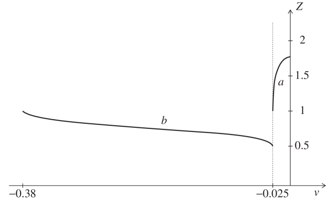
FIG. 11.: Dressed charge as a function of ledge chemical potential for two points in the ($\gamma,\omega$)-plane.

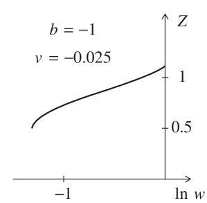
FIG. 12.: (a) Dressed charge as a function of ledge interaction for fixed values of ledge stiffness $w$ and chemical potential $v$ (b) Dressed charge as a function of $\ln w$ for fixed $b$ and $v$.

Since the correlation functions in which we are interested contain only operators which conserve the number of particles, we can restrict ourselves to $\Delta M=0$. We then obtain the following form for the asymptotics of the height-difference correlation function

$$C^{c}(x,y)=\frac{A}{x^{2}+v_{F}^{2}y^{2}}+\frac{B\cos(2p_{F}x)}{(x^{2}+v_{F}^{2}y^{2})^{Z^{2}}}.$$ (51)

It is useful to recast (51) in a slightly different form. We consider a line in the $(v_{F}\sin\theta,\cos\theta)$ direction ($\theta=0$ is vertical, $\theta=\pi/2$ is horizontal) and define a height function $h_{\theta}(r)=h(rv_{F}\sin\theta,r\cos\theta)$. In the scaling limit height-differences become derivatives. Thus, we expect the lattice equivalent of $h_{\theta}^{\prime}=dh_{\theta}(r)/dr$ to be $\frac{\cos\theta+v_{F}\sin\theta}{2}d_{+}+\frac{\cos\theta-v_{F}\sin\theta}{2}d_{-}$, which in turn implies the following form for the connected correlation function in radial coordinates

$$C^{c}_{\theta}(r_{2}-r_{1})=\left\langle h_{\theta}^{\prime}(r_{1})h_{\theta}^{\prime}(r_{2})\right\rangle=A_{\theta}|r_{2}-r_{1}|^{-2}+B_{\theta}\cos(2p_{F}v_{F}|r_{2}-r_{1}|\sin\theta)r^{-2Z^{2}}\ .$$ (52)

Here $A_{\theta}$ and $B_{\theta}$ are quadratic forms in $\cos\theta\pm v_{F}\sin\theta$, i.e. affine functions of $\cos 2\theta$ and $\sin 2\theta$.

$C^{c}_{\theta}(r)$ is related to the height correlation function

$$H^{c}_{\theta}(r_{2}-r_{1})=\left\langle\left(h_{\theta}(r_{1})-h_{\theta}(r_{2})-\frac{D}{2}(r_{1}-r_{2})v_{F}\sin\theta\right)^{2}\right\rangle$$ (53)

by

$$C^{c}_{\theta}(r)=-\frac{d^{2}H^{c}_{\theta}(r)}{dr^{2}}$$ (54)

therefore the asymptotic behaviour of $H$ is

$$H^{c}_{\theta}(r)=A_{\theta}\ln r+\frac{B_{\theta}}{4p_{F}^{2}v_{F}^{2}\sin^{2}\theta}\frac{\cos(2p_{F}v_{F}r\sin\theta)}{r^{2Z^{2}}}+E_{\theta}r+F_{\theta}$$ (55)

We believe that $E_{\theta}=0$ for any value of $\theta$. We have already seen that $E_{\pi/2}=0$.

As $\theta\to 0$ the amplitude of the $r^{-2Z^{2}}$ term is expected to diverge. We cannot prove this since $B_{\theta}$ might be proportional to $(1-\cos 2\theta)$, but we have no reason to believe that this is the case.

VIII Discussion

The results of [2] were mainly of a thermodynamic character. In the half-filling case, corresponding to a tilt angle of $\pi/4$, there is a phase transition at $e^{b}=(1-w)^{2}$ for the case of repulsive interactions $b<0$. This is of Kosterlitz-Thouless, or equivalently, Lieb-F type. For tilt angles $0<\theta<\theta_{f}$ which differ from $\pi/4$, there is no thermodynamic singularity. For $\theta=\pi/4$ and small enough temperature, a Peierls proof along the lines of Brascamp et al. [30] shows that the fluctuations in height about the $\theta=\pi/4$ surface are of order one, whereas in the free-Fermi case $e^{b}=1-w^{2}$ (see appendix B), there are logarithmic height fluctuations, as in the BCSOS model, which also has a free-Fermion point.

The interesting question is what happens for $\theta\neq\pi/4$ at a level of correlation functions. We show that for $\theta\neq\pi/4$ and no binding of ledges, the excitation spectrum is gapless. This gives a power-law decay of height step-step correlation functions by using conformal arguments. In addition to the $r^{-2}$ term which leads to logarithmic height fluctuations, we find an oscillatory term which decays algebraicly with a nonuniversal exponent, but whose contribution to height fluctuations is subdominant.

At $\theta=\pi/4$ and below the transition temperature, the transfer-matrix spectrum has a gap, giving exponential decay of correlations of local objects.

There is another phase transition which occurs for any angle $0<\theta<\theta_{f}$ at the solution of $e^{b}=(1+w)^{2}$. This has zero limiting entropy per unit basal area below the transition temperature $T_{c}$, and a specific heat which diverges as $(T-T_{c})^{-1/2}$ from above. In this high-temperature phase, we have gapless excitations as before, and therefore a rough surface. This phase transition may be thought of as of pinning-depinning type. The low-temperature phase has a complete collapse of the ledges in a close-packed strip with axis in the Euclidean time direction. We have not analysed the correlation functions in this case. We must point out that the results in this part of the phase diagram are almost certainly critically dependent on the nature of the short-range interactions.

In appendix E, the interaction between two ledges separated by mean distance $l$ is found to have the same $l^{-2}$ behaviour as the law which would be obtained from elastic theory or from the interaction between electrostatic dipoles located along the ledges, which may be approximated by pairwise interactions between neighbouring edges. Our model gives a consistent treatment of that part of the elastic interaction which comes from deformation of the surface via entropic interactions. This part tends to zero as the temperature $T\to 0$. But the dipole term does not vanish in the same limit and thus, when present, should dominate the low-temperature behaviour. Thus we believe that the model considered by Villain et al. [11] for sections vicinal to Cu(111) is fundamentally different; our model only shows roughening at the unique half-filling angle of tilt, thermodynamically speaking, and the microscopic picture strongly supports this view. For less-than-half filling, there is extensive degeneracy because of the form of the short-range interaction in our basic model. One might then ask why the $1/l^{2}$ entropic repulsion which comes in at the coarse-grained level does not break this degeneracy, for any $T>0$ (at zero temperature this interaction vanishes), and thereby produce a phase transition. Clearly a better understanding of this is needed.

The recent work on vicinal surfaces of ${}^{4}{\rm He}$ crystals [31] suggests that there may be a critical tilt angle of the vicinal section, below which neighbouring ledges are rather straight and thus do not overlap, but above which the ledges wander sufficiently to come into close contact. In our model, such a critical angle does not appear in the thermodynamics. However, in order to address the questions raised by the experiments [31], it may be necessary to study the behaviour of ledges at a microscopic level, and possibly also to take into account defects and boundaries. Examples are known [32] of pair functions near surfaces with weakened bonds where there is a transition behaviour in the asymptotics, but, on applying a fluctuation sum formula to get a derivative of the free energy, no thermodynamic singularity is seen. Thus caution is advisable in drawing conclusions from the thermodynamics alone.

IX Acknowledgments

We are grateful to B. Duplantier, T. L. Einstein, M. Gaudin, J. M. Luck, A. E. Malevanets and N. Mousseau for interesting discussions.

We acknowledge financial support from EPSRC under grant number GR/K97783.

A A commuting family of transfer matrices for the TLK model

In this appendix we construct an embedding of the TLK model into the framework of the Quantum Inverse Scattering Method [18]. We then show how to recover the coordinate Bethe Ansatz solution of [2]. The vertices in the diagonal-to-diagonal formulation of the TLK model are given by (5). We define a diagonal-to-diagonal transfer matrix as follows

$$U_{2N}=R^{\beta_{2}\beta_{3}}_{\alpha_{1}\alpha_{2}}R^{\beta_{4}\beta_{5}}_{\alpha_{3}\alpha_{4}}\ldots R^{\beta_{2N}\beta_{1}}_{\alpha_{2N-1}\alpha_{2N}}\ .$$ (A1)

We note that the square of this transfer matrix commutes with the square of the translation operator $\tau_{R}$

$$[U_{2N}^{2},\tau_{R}^{2}]=0\ .$$ (A2)

The transfer matrix $\tau_{dd}$ studied in [2] is expressed as

$$\tau_{dd}=\tau_{R}^{2}\ U_{2N}^{2}\ ,$$ (A3)

and the partition function of the TLK model is given by

$$Z={\rm Trace}\left(\tau_{dd}\right)^{L}\ .$$ (A4)

Correlation functions can also be expressed in terms of $\tau_{dd}$ so that the problem of solving the TLK model reduces to the one of finding eigenvalues and eigenvectors of $\tau_{dd}$.

Following [33] we can reformulate the problem in terms of an inhomogeneous row-to-row transfer matrix of a 6-vertex model in a vertical electric field [20]. Starting point is the usual XXZ (symmetric 6-vertex) $L$-operator [18]

$$L_{n}(\lambda)=\left(\begin{array}[]{cc}\frac{\sinh(\lambda+i\frac{\gamma}{2}\sigma_{n}^{z})}{i\sin\gamma}&\sigma_{n}^{-}\\[8.0pt] \sigma_{n}^{+}&\frac{\sinh(\lambda-i\frac{\gamma}{2}\sigma_{n}^{z})}{i\sin\gamma}\end{array}\right).$$ (A5)

Here $\Gamma$ is a free parameter and $\sigma^{\alpha}$ are the usual Pauli matrices. Note that there exists a so-called shift point at $\lambda=i\frac{\gamma}{2}$ (at which the L-operator reduces to the permutation operator), i.e.

$$L_{n}(i\frac{\gamma}{2})=\left(\begin{array}[]{cc}\frac{1}{2}(1+\sigma^{z}_{n})&\sigma_{n}^{-}\\[8.0pt] \sigma_{n}^{+}&\frac{1}{2}(1-\sigma^{z}_{n})\end{array}\right).$$ (A6)

The L-operator of the model with a vertical field is then simply

$${\cal L}_{n}(\lambda)=\exp(\frac{v}{2}\sigma^{z}_{n})L_{n}(\lambda)\exp(\frac{v}{2}\sigma^{z}_{n})\ .$$ (A7)

Consider now an inhomogeneous row-to-row transfer matrix of such an asymmetric 6-vertex model on a lattice with $2N$ sites

$${\cal T}(\mu) = {\rm Trace}\ {\cal L}_{2N}(\mu-i\frac{\omega}{2}){\cal L}_{2N-1}(\mu){\cal L}_{2N-2}(\mu-i\frac{\omega}{2}){\cal L}_{2N-3}(\mu)\ldots{\cal L}_{2}(\mu-i\frac{\omega}{2}){\cal L}_{1}(\mu)$$ (A8)

$$\equiv {\rm Trace}\ \exp(\frac{v}{2}\sum_{n}\sigma^{z}_{n})T(\mu)\exp(\frac{v}{2}\sum_{n}\sigma^{z}_{n})\ ,$$ (A9)

where $T(\mu)$ is the symmetric inhomogeneous 6-vertex transfer matrix constructed from the L-operators $L_{n}(\lambda)$. Here the inhomogeneity $\Omega$ is a second free parameter. Choosing $\mu=i\frac{\gamma}{2}$ and using (A6) we find

$${\cal T}(i\frac{\gamma}{2})=\left(\widehat{{\cal L}}_{2N}(i\frac{\gamma}{2}-i\frac{\omega}{2})\right)^{\alpha_{1}\beta_{2N-1}}_{\alpha_{2N}\ b_{2N}}\left(\widehat{{\cal L}}_{2N-2}(i\frac{\gamma}{2}-i\frac{\omega}{2})\right)^{\alpha_{2N-1}\beta_{2N-3}}_{\alpha_{2N-2}\beta_{2N-2}}\ldots\left(\widehat{{\cal L}}_{2}(i\frac{\gamma}{2}-i\frac{\omega}{2})\right)^{\alpha_{3}\beta_{1}}_{\alpha_{2}\beta_{2}}\ ,$$ (A10)

where

$$\widehat{{\cal L}}_{2N}(i\frac{\gamma-\omega}{2})=\left(\begin{array}[]{cccc}e^{2v}\frac{\sin({\gamma}-\frac{\omega}{2})}{\sin{\gamma}}&&&\\[8.0pt] &-\frac{\sin\frac{\omega}{2}}{\sin{\gamma}}&1&\\[8.0pt] &1&-\frac{\sin\frac{\omega}{2}}{\sin{\gamma}}&\\[8.0pt] &&&e^{-2v}\frac{\sin({\gamma}-\frac{\omega}{2})}{\sin{\gamma}}\end{array}\right).$$ (A11)

It follows that the inhomogeneous row-to-row transfer matrix is identical to the diagonal-to-diagonal transfer matrix if we make the following identifications

$$e^{-2v}\frac{\sin({\gamma}-\frac{\omega}{2})}{\sin{\gamma}}=e^{-a}\ ,\quad-\frac{\sin\frac{\omega}{2}}{\sin{\gamma}}=w\ ,\quad\left(\frac{\sin({\gamma}-\frac{\omega}{2})}{\sin{\gamma}}\right)^{2}=e^{b}\ .$$ (A12)

Note that $4v=b+2a$. Consider now an eigenstate of $T(\mu)$ (the transfer matrix of the inhomogeneous, symmetric 6-vertex model) with eigenvalue $\nu(\mu)$

$$T(\mu)|\Lambda\rangle=\nu(\mu)|\Lambda\rangle\ .$$ (A13)

Then, because the $z$-component of total spin is a good quantum number, we have

$${\cal T}(\mu)|\Lambda\rangle=e^{v(N_{\uparrow}-N_{\downarrow})}\nu(\mu)|\Lambda\rangle\ ,$$ (A14)

where $N_{\uparrow,\downarrow}$ are the total numbers of up up/down spins in the state $|\Lambda\rangle$. This means that we can obtain a complete set of eigenstates of ${\cal T}(\mu)$ from a complete set of eigenstates of $T(\mu)$. The eigenvalues of $T(\mu)$ are given by (we choose the state with all spins down as the reference state)

$$\nu(\mu) = \left(\frac{\sinh(\mu-i\frac{\omega}{2}-i\frac{\gamma}{2})\sinh(\mu-i\frac{\gamma}{2})}{-\sin^{2}\gamma}\right)^{N}\prod_{j=1}^{M}\frac{\sinh(\mu-\lambda_{j}+i\gamma)}{\sinh(\mu-\lambda_{j})}$$ (A15)

$$+ \left(\frac{\sinh(\mu-i\frac{\omega}{2}+i\frac{\gamma}{2})\sinh(\mu+i\frac{\gamma}{2})}{-\sin^{2}\gamma}\right)^{N}\prod_{j=1}^{M}\frac{\sinh(\mu-\lambda_{j}-i\gamma)}{\sinh(\mu-\lambda_{j})}\ ,$$ (A16)

where $M=N_{\uparrow}$ and where the spectral parameters $\lambda_{j}$ are solutions of the Bethe Ansatz equations

$$\left(\frac{\sinh\left(\lambda_{k}+i\frac{\gamma}{2}\right)}{\sinh\left(\lambda_{k}-i\frac{\gamma}{2}\right)}\ \frac{\sinh\left(\lambda_{k}-i\frac{\omega-\gamma}{2}\right)}{\sinh\left(\lambda_{k}-i\frac{\omega+\gamma}{2}\right)}\right)^{N}=-\prod_{j=1}^{M}\frac{\sinh\left(\lambda_{k}-\lambda_{j}+i{\gamma}\right)}{\sinh\left(\lambda_{k}-\lambda_{j}-i{\gamma}\right)}\ ,\ k=1\ldots M\ .$$ (A17)

We thus find that the eigenvalues of $U_{2N}={\cal T}(\frac{i\gamma}{2})$ are given by

$$\Lambda(\{\lambda_{j}\})=e^{a(M-N)}\left(\frac{\sin(\gamma-\frac{\omega}{2})}{\sin\gamma}\right)^{M}\prod_{j=1}^{M}\frac{\sinh\left(\lambda_{j}+i\frac{\gamma}{2}\right)}{\sinh\left(\lambda_{j}-i\frac{\gamma}{2}\right)}\ .$$ (A18)

In order to make contact with the results obtained in [2] we need to consider the transfer matrix $\tau_{dd}=\tau_{R}^{2}U_{2N}^{2}$. From the standard construction of [18] it follows that the eigenvalues of the operator of translation by two sites $\tau_{R}^{2}$ are given by

$$\exp\left(ip(\{\lambda_{j}\})\right)=\prod_{k=1}^{M}\frac{\sinh\left(\lambda_{k}-i\frac{\gamma}{2}\right)}{\sinh\left(\lambda_{k}+i\frac{\gamma}{2}\right)}\ \frac{\sinh\left(\lambda_{k}-i\frac{\omega+\gamma}{2}\right)}{\sinh\left(\lambda_{k}-i\frac{\omega-\gamma}{2}\right)}\ .$$ (A19)

This then implies that the eigenvalues $\Lambda_{dd}$ of $\tau_{dd}$ are

$$\Lambda_{dd}(\{\lambda_{j}\})=e^{2a(M-N)}\left(\frac{\sin(\gamma-\frac{\omega}{2})}{\sin\gamma}\right)^{2M}\prod_{j=1}^{M}\frac{\sinh\left(\lambda_{j}+i\frac{\gamma}{2}\right)}{\sinh\left(\lambda_{j}-i\frac{\gamma}{2}\right)}\frac{\sinh\left(\lambda_{j}-i\frac{\gamma+\omega}{2}\right)}{\sinh\left(\lambda_{j}+i\frac{\gamma-\omega}{2}\right)}\ .$$ (A20)

Equations (A17) and (A20) are equivalent to (11) and (9) of [2] if we set $a=0$ and substitute the function $s(k)$ of [2] by

$$s(k)=\frac{\sinh(\lambda-i\omega/2+i\gamma/2)}{\sinh(\lambda-i\gamma/2)}=\frac{\exp(2\lambda+i\gamma-i\omega/2)-\exp(i\omega/2)}{\exp(2\lambda)-\exp(i\gamma)}\ .$$ (A21)

B Free-fermion cases

For $\gamma=\pi/2$ the two-particle scattering phase shifts on the right hand side of (7) reduce to $-1$: the particles are free fermions. This corresponds to the following constraint on the weights: $e^{b}=1-w^{2}$. The model is physical only if $e^{b}$ and $w$ are real and positive. This implies that $b$ is negative: the interaction between ledges is repulsive.

The Bethe Ansatz equations (A17) become

$$\left(\frac{\sinh(\lambda_{k}+i\gamma/2)\sinh(\lambda_{k}-i\omega/2+i\gamma/2)}{\sinh(\lambda_{k}-i\gamma/2)\sinh(\lambda_{k}-i\omega/2-i\gamma/2)}\right)^{N}=(-)^{M-1}$$ (B1)

Clearly the rapidities $\lambda_{k}$ are constrained to lie on the lines $\Im m\lambda=i\omega/4$ and $\Im m\lambda=i\omega/4+i\pi/2$, which we denote by ${\cal C}_{1}$ and ${\cal C}_{2}$ respectively. The state corresponding to the largest eigenvalue of the transfer matrix $\tau_{dd}$ is then obtained by filling a Fermi sea of (occupied) rapidities on one of these lines. We distinguish two cases:

• $w\coth 2v<-1$:

  In this case there is a Fermi sea on ${\cal C}_{2}$ with Fermi level given by $\cosh 2\lambda_{F}=-w\coth 2v$. The line ${\cal C}_{1}$ is empty. This is a critical phase with power-law correlations.

• $-1<w\coth 2v<0$:

  In this case the reference state itself (i.e. the state with all spins down) corresponds to the largest eigenvalue: both lines ${\cal C}_{j}$ are empty. This phase is in general massive i.e. the next-largest eigenvalue of $\tau_{dd}$ is separated from the largest one by a gap. Accordingly correlations are characterized by an exponential decay.

Note that for $v>0$ the state with all spins up can be used as reference state; the distribution of rapidities is then given by the same rule as above but with $v$ changed to $-v$. (We do not consider this case any further.)

For any $0<w<1$ all regimes can be reached by varying $a$. For $v=0$, i.e. $a=-b/2$, the number of ledges in the ground state is $M=N$. In order to study correlation functions it is convenient to switch to the “coordinate-space” notation of [2]. We define a “particle momentum” $k$ and two functions $s_{\pm}(k)$ by

$$e^{ik} = \frac{\sinh(\lambda+i\gamma/2)\sinh(\lambda-i\omega/2+i\gamma/2)}{\sinh(\lambda-i\gamma/2)\sinh(\lambda-i\omega/2-i\gamma/2)},$$ (B2)

$$s_{\pm}(k) = \frac{w(e^{ik}-1)}{2}\pm e^{ik/2}\sqrt{1-w^{2}\sin^{2}k/2}.$$ (B3)

We then construct fermionic creation and annihilation operators by means of a Jordan-Wigner transformation on the spin variables defining the vertex model

$$c_{j}^{+}=(-\sigma_{1}^{z})(-\sigma_{2}^{z})\dots(-\sigma_{j-1}^{z})\frac{\sigma_{j}^{x}+i\sigma_{j}^{y}}{2}.$$ (B4)

In the momentum-space representation there are two “bands” of fermions with momentum $k$ because rapidities on ${\cal C}_{1}$ and ${\cal C}_{2}$ with equal real parts correspond to the same value of $k$. Fermion annihilation and creation operators are of the form

$$C_{\pm}(k) = \sqrt{\frac{2}{N}}\frac{1}{s_{\mp}(k)-s_{\pm}(k)}\left(\sum\limits_{j=1}^{N}e^{-ikj}s_{\mp}(k)c_{2j}-\sum\limits_{j=0}^{N-1}e^{-ikj}c_{2j+1}\right),$$ (B5)

$$C_{\pm}^{\dagger}(k) = \frac{1}{\sqrt{2N}}\left(\sum\limits_{j=1}^{N}e^{ikj}c_{2j}^{+}+\sum\limits_{j=0}^{N-1}e^{ikj}s_{\pm}(k)c_{2j+1}^{+}\right).$$ (B6)

The inverse relation between momentum-space and position-space operators is

$$c_{2j}=\frac{1}{\sqrt{2N}}\sum_{k,\alpha}e^{ikj}C_{k,\alpha} c_{2j+1}=\frac{1}{\sqrt{2N}}\sum_{k,\alpha}s_{\alpha}(k)e^{ikj}C_{k,\alpha}$$ (B7)

$$c_{2j}^{+}=\sqrt{\frac{2}{N}}\sum_{k,\alpha}\frac{s_{-\alpha}(k)}{s_{-\alpha}(k)-s_{\alpha}(k)}e^{-ikj}C_{k,\alpha}^{\dagger} c_{2j+1}^{+}=\sqrt{\frac{2}{N}}\sum_{k,\alpha}\frac{e^{-ikj}}{s_{\alpha}(k)-s_{-\alpha}(k)}C_{k,\alpha}^{\dagger}\ .$$ (B8)

The vacuum state of the fermionic Fock space is defined by $C_{k,\pm}|\Omega\rangle=0$. Eigenstates of the transfer matrix are obtained by acting with creation operators $C^{\dagger}_{k,\pm}$ on the vacuum

$$|k_{1}\ldots k_{n}|\alpha_{1}\ldots\alpha_{n}\rangle=\prod_{j=1}^{n}C^{\dagger}_{k_{j},\alpha_{j}}|\Omega\rangle\ .$$ (B9)

The corresponding eigenvalue of the transfer matrix is

$$\tau_{dd}|k_{1}\ldots k_{n}|\alpha_{1}\ldots\alpha_{n}\rangle=\prod_{j=1}^{n}e^{2a}[1+w\ s_{\alpha_{j}}(k_{j})][1+w/s_{\alpha_{j}}(k_{j})]\ |k_{1}\ldots k_{n}|\alpha_{1}\ldots\alpha_{n}\rangle\ .$$ (B10)

In terms of the $k,\alpha$ variables the maximal eigenvalue of the transfer matrix corresponds to the state $|0\rangle$ defined by filling a Fermi sea in the $+$ band between the Fermi points $-k_{F}$ and $k_{F}$, i.e.

$$|0\rangle=\prod_{|k|\leq k_{F}}C^{\dagger}_{+}(k)|\Omega\rangle\ .$$ (B11)

Let us now turn to the calculation of correlation functions. using standard free-fermion methods we can derive integral representations for the correlation functions of height differences. However, we shall see that the results are much more complicated than for the case of the BCSOS model [6, 34].

1 Correlators of height-differences in $y$-direction

The height difference in $y$-direction is given by $d_{y}(x,2y)=h(x,2y+1)-h(x,2y-1)$, where $x$ is a half-odd-integer. The corresponding operator for $x=3/2$ is given by

$$(\delta_{y}(3/2))^{\alpha_{1}\ldots\alpha_{2N}}_{\alpha^{\prime}_{1}\ldots\alpha^{\prime}_{2N}} = A^{\alpha_{1}\alpha_{2}}_{\alpha^{\prime}_{1}\alpha^{\prime}_{2}}\prod_{j=3}^{2N}\delta^{\alpha_{j}}_{\alpha^{\prime}_{j}},$$ (B12)

where the nonzero elements of $A$ are

$$A^{12}_{21}=\frac{w}{1-w^{2}},\qquad A^{21}_{12}=-\frac{w}{1-w^{2}},\qquad A^{12}_{12}=\frac{w^{2}}{1-w^{2}},\qquad A^{21}_{21}=-\frac{w^{2}}{1-w^{2}}.$$ (B13)

The correlation function of the height differences (for even separations) is then given by

$$C_{yy}(2x,2y) = \langle d_{y}(2x_{0}-1/2,2y_{0}-1)d_{y}(2x_{0}-1/2+2x,2y_{0}-1+2y)\rangle$$ (B14)

$$= {\rm Trace}\left(\tau_{dd}^{L-y}\delta_{y}(3/2)\tau_{dd}^{y}\tau_{R}^{2x}\delta_{y}(3/2)\tau_{R}^{-2x}\right).$$ (B15)

We note that this formula is valid only for $y>0$. formula The operator (B12) can be expressed in terms of the fermion operators as

$$\delta_{y}(3/2) = \frac{1}{N}\sum_{k_{1},k_{2},\alpha_{1},\alpha_{2}}a_{\alpha_{1},\alpha_{2}}(k_{1},k_{2})\ C_{\alpha_{2}}^{\dagger}(k_{2})\ C_{\alpha_{1}}(k_{1})\ ,$$ (B16)

where

$$a_{\alpha_{1},\alpha_{2}}(k_{1},k_{2})=\frac{w\ s_{\alpha_{1}}(k_{1})+we^{ik_{1}-ik_{2}}s_{\alpha_{2}}(k_{2})+e^{ik_{1}}+s_{\alpha_{1}}(k_{1})s_{\alpha_{2}}(k_{2})}{(w-w^{-1})(s_{\alpha_{2}}(k_{2})-s_{-\alpha_{2}}(k_{2}))}\ .$$ (B17)

This yields the following representation for the correlation function of height-differences

$$C_{yy}(2x,2y)=\frac{1}{N^{2}}\sum_{{\rm hole}(k_{h},+),{\rm particle}(k_{p},\alpha)}a_{+,\alpha}(k_{h},k_{p})\ a_{\alpha,+}(k_{p},k_{h})\ \left(\Lambda_{\alpha}(k_{p})/\Lambda_{+}(k_{h})\right)^{y}e^{ix(k_{p}-k_{h})}.$$ (B18)

Here the sum extends over all holes with momentum $k_{h}$ in the Fermi sea in the $+$ band ($|k_{h}|\leq k_{F}$) and all particles in either the $+$ band ($\pi\geq|k_{p}|>k_{F}$, $\alpha=+$) or the $-$ band ($|k_{p}|\leq\pi$, $\alpha=-$) and

$$\Lambda_{\alpha}(k)=e^{2a}[1+w\ s_{\alpha}(k)][1+w/s_{\alpha}(k)]\ .$$ (B19)

In the thermodynamic limit we obtain the following integral representation

$$C_{yy}(2x,2y) = \int_{-k_{F}}^{k_{F}}dk_{h}\left\{\int_{k_{F}}^{\pi}+\int_{-\pi}^{-k_{F}}dk_{p}\right\}a_{+,+}(k_{h},k_{p})\ a_{+,+}(k_{p},k_{h})$$ (B21)

$$\left(\frac{w\cos(k_{p}/2)+\sqrt{1-w^{2}\sin^{2}(k_{p}/2)}}{w\cos(k_{h}/2)+\sqrt{1-w^{2}\sin^{2}(k_{h}/2)}}\right)^{2y}e^{ix(k_{p}-k_{h})}$$

$$+ \int_{-k_{F}}^{k_{F}}dk_{h}\int_{-\pi}^{\pi}dk_{p}\ a_{+,-}(k_{h},k_{p})\ a_{-,+}(k_{p},k_{h})$$ (B23)

$$\left(\frac{w\cos(k_{p}/2)-\sqrt{1-w^{2}\sin^{2}(k_{p}/2)}}{w\cos(k_{h}/2)-\sqrt{1-w^{2}\sin^{2}(k_{h}/2)}}\right)^{2y}e^{ix(k_{p}-k_{h})}\ .$$

We have not managed to greatly simplify (B23). However, it is straightforward to extract the asymptotic behaviour for $z\to\infty$ by expanding the integrand around the maxima at $k_{h},k_{p}=\pm k_{F}$.

2 Correlators of height-differences in $x$-direction

The height difference in $x$-direction $d_{x}(1,2y-1)=h(3/2,2y-1)-h(1/2,2y-1)$ is measured by the operator

$$\delta_{x}(1) = c_{1}^{-}c_{1}^{+}=\frac{1}{N}\sum_{k_{1},k_{2},\alpha_{1},\alpha_{2}}\frac{s_{\alpha_{1}}(k_{1})}{s_{\alpha_{2}}(k_{2})-s_{-\alpha_{2}}(k_{2})}C_{\alpha_{2}}^{\dagger}(k_{2})\ C_{\alpha_{1}}(k_{1})\ .$$ (B24)

The corresponding correlation function of height differences (for even separations) has the following integral representation

$$C_{xx}(2x,2y) = \int_{-k_{F}}^{k_{F}}dk_{h}\left\{\int_{k_{F}}^{\pi}+\int_{-\pi}^{-k_{F}}dk_{p}\right\}\frac{s_{+}(k_{h})}{s_{+}(k_{p})-s_{-}(k_{p})}\frac{s_{+}(k_{p})}{s_{+}(k_{h})-s_{-}(k_{h})}$$ (B26)

$$\left(\frac{w\cos(k_{p}/2)+\sqrt{1-w^{2}\sin^{2}(k_{p}/2)}}{w\cos(k_{h}/2)+\sqrt{1-w^{2}\sin^{2}(k_{h}/2)}}\right)^{2y}e^{ix(k_{p}-k_{h})}$$

$$+ \int_{-k_{F}}^{k_{F}}dk_{h}\int_{-\pi}^{\pi}dk_{p}\ \frac{s_{+}(k_{h})}{s_{-}(k_{p})-s_{+}(k_{p})}\frac{s_{-}(k_{p})}{s_{+}(k_{h})-s_{-}(k_{h})}$$ (B28)

$$\left(\frac{w\cos(k_{p}/2)-\sqrt{1-w^{2}\sin^{2}(k_{p}/2)}}{w\cos(k_{h}/2)-\sqrt{1-w^{2}\sin^{2}(k_{h}/2)}}\right)^{2y}e^{ix(k_{p}-k_{h})}\ .$$

3 Height-correlations along the $y$-direction

Above we have derived integral representations for the (local) correlation functions of height-differences. In the remainder of this appendix we consider height-correlations along the transfer direction. The height correlation function $H(0,y)=\langle(h(3/2,2y)-h(3/2,0))^{2}\rangle$ is related to $C_{yy}(0,y)$ by

$$H(0,2y+2)+H(0,2y-2)-2H(0,2y)=2C_{yy}(0,2y),$$ (B29)

where $H(0,0)=0$ and $H(0,2)=C_{yy}(0,0)$. Summing (B29) we find that

$$C_{yy}(0,0)+2\sum_{z=1}^{y-1}C_{yy}(0,2z)=H(0,2y)-H(0,2y-2).$$ (B30)

The algebraic decay $C_{yy}(0,2y)\propto\frac{A}{y^{2}}$ of the height-difference correlation functions implies that the surface is rough

$$H(0,2y)\propto F+E_{y}\ y+A^{\prime}\ \ln y+\ldots\ ,$$ (B31)

where in the thermodynamic limit

$$E_{y}=C_{yy}(0,0)+2\sum_{y=1}^{\infty}C_{yy}(0,2y)\ .$$ (B32)

On physical grounds we expect that $E_{y}=0$ as we now argue. Let us define a variable $D_{y}=\sum_{y=1}^{N}d_{y}(x,2y)$ in our finite $2N\times 2L$-toroidal geometry. $D_{y}$ is independent of $x$ because $d_{x}(x+1/2,y)=h(x+1,y)-h(x,y)$ is subject to periodic boundary conditions. $E_{y}$ and $D_{y}$ are related by

$$E_{y}=\lim_{N,L\rightarrow\infty}\left\langle d_{y}(x,y)D_{y}\right\rangle=\lim_{N,L\rightarrow\infty}\frac{\left\langle D_{y}^{2}\right\rangle}{L}.$$ (B33)

The average tilt of ledges in the $xy$-plane is $s=(ND_{y})/(LM)$: for instance if $D_{y}=0$ the ledges are on average parallel to the transfer direction ($s=0$). Phenomenologically we expect that ledges have a stiffness $\Sigma$, so that the total energy cost of a nonzero $D_{y}$, i.e. of a nonzero $s$ is roughly $\Sigma LMs^{2}/2$, at least for $s\ll 1$. The equipartition theorem then gives that the average value of $s^{2}$ should be of order $(NM)^{-1}$. This implies that $E_{y}=0$ provided that in thermodynamic limit $N^{2}$ increases faster than the number of ledges $M$. This condition is satisfied whenever the ground state is described by a finite density function, with $M/N$ finite.

For the special case at hand we have explicitly verified that $E_{y}=0$: Inserting (B18) together with

$$C_{yy}(0,0)=\langle 0|(w-w^{-1})\left\{{wc_{1}^{+}c_{1}c_{2}c_{2}^{+}+wc_{1}c_{1}^{+}c_{2}^{+}c_{2}+c_{1}c_{2}^{+}-c_{1}^{+}c_{2}}\right\}|0\rangle.$$ (B34)

into (B32) we obtain

$$E_{y}(k_{F}) = -\frac{\left\langle 0\right|c_{2}^{+}c_{1}+c_{1}^{+}c_{2}\left|0\right\rangle}{w-w^{-1}}$$ (B36)

$$+\frac{1}{N^{2}}\sum_{{\rm hole}(k_{h},+),{\rm particle}(k_{p},\alpha)}a_{+,\alpha}(k_{h},k_{p})a_{\alpha,+}(k_{p},k_{h})\frac{\Lambda_{+}({k_{h}})+\Lambda_{\alpha}{(k_{p})}}{\Lambda_{+}({k_{h}})-\Lambda_{\alpha}{(k_{p})}}\ ,$$

where we have explicitly displayed the dependence on the Fermi momentum $k_{F}$. By inspection we see that

$$E_{y}(0)=0\ .$$ (B37)

Rather than trying to evaluate (B36) directly, we calculate the change $N\delta E_{y}(k_{F})=N(E_{y}(k_{F}+\delta k_{F})-E_{y}(k_{F}))$ under a change of Fermi momentum $\delta k_{F}=2\pi N^{-1}$

$$N\delta E_{y}(k_{F}) = \frac{2}{w^{-1}-w}\frac{1+e^{ik_{F}}}{s_{+,F}-s_{-,F}}$$ (B40)

$$+\frac{1}{N}\sum\limits_{-\pi<k<\pi}\left(a_{+,+}(k_{F},k)a_{+,+}(k,k_{F})+a_{+,+}(-k_{F},k)a_{+,+}(k,-k_{F})\right)\frac{\Lambda_{+}(k_{F})+\Lambda_{+}(k)}{\Lambda_{+}(k_{F})-\Lambda_{+}(k)}$$

$$+\frac{1}{N}\sum\limits_{-\pi<k<\pi}\left(a_{+,-}(k_{F},k)a_{-+}(k,k_{F})+a_{+,-}(-k_{F},k)a_{-+}(k,-k_{F})\right)\frac{\Lambda_{+}(k_{F})+\Lambda_{-}(k)}{\Lambda_{+}(k_{F})-\Lambda_{-}(k)}\ .$$

Turning the sums into integrals and integrating numerically we find that this is indeed zero. Alternatively, if we perform the sums for large finite $N$ we find that the right hand side of (B40) scales like $1/N$. In conjunction with (B37) this shows that $E_{y}$ is indeed zero.

C The case of negative kink energy

In this appendix we discuss the case $w>1$.

This corresponds to the following extensions of the regions discussed earlier: Region (1a) with $-2\pi<\omega<-2\gamma$; Region (1b) with $-2\pi<\omega<-2\pi+2\gamma$; Region (2) with $\omega<-2\gamma$; Region (3) with $\omega>2\gamma$. In all cases the one-particle spectrum is quite different from the results obtained for $w<1$. In addition to the lines in spectral parameter space discussed above, we find that there are curves on which the bare momentum is real and the bare energy has a constant real part but acquires a variable imaginary part (whereas both bare momentum and bare energy remain real on the straight lines).

We specialize the remainder of this discussion to Region (3). The curves, shown on Fig. 13, are parametrized by $\lambda=x+iy+i\omega/4$ with $x$ and $y$ real and satisfying:

$$\cosh\gamma\cosh(2y)=\cosh(\omega/2)\cos(2x).$$ (C1)

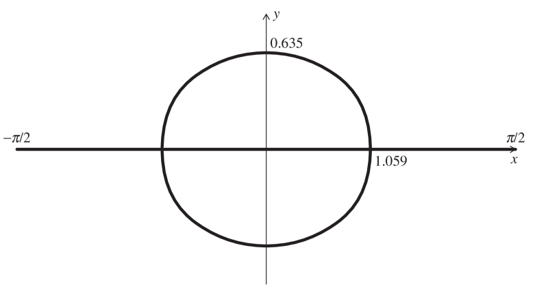
FIG. 13.: Location of one-strings in the $(x,y)$ plane with $\lambda=x+iy+i\omega/4$, for $\gamma=1$ and $\omega=5$.

The line corresponds to low-momentum states $-p_{c}<p_{0}<p_{c}$, and the curves to high-momentum states $|p_{0}|>p_{c}$ ($p_{c}$ is comprised between $0$ and $\pi$ and depends on the parameters $\gamma$ and $\omega$). If we consider the dispersion relation, i.e. the (bare) energy as a function of (bare) momentum, there are branch points which correspond to the contact point between the line and the curves in term of the spectral parameter. For the high-momentum states the bare energy becomes complex, and its real part is constant on the whole, equal to the energy at the contact point.

We first describe the maximum-eigenvalue state. We believe that this state is made up of particles with spectral parameters $\lambda_{k}=x_{k}+i\omega/4$, where all $x_{k}$ are real. However the situation is different from that considered in the main text in one important aspect: for $\omega>2\gamma$ we find that the bare momentum is not a monotonous function of $x$, so that the bare density $\rho_{0}(x)=\frac{1}{2\pi}dp_{0}/dx$ is not positive: it turns out that its average value vanishes.

The logarithm of the Bethe Ansatz equations is:

$$Np_{0}(x_{k})-\sum_{j}\theta(x_{k}-x_{j})=\pi+2\pi I_{k}$$ (C2)

where

$$e^{i\theta(x)}=\frac{\sinh(x+i\gamma)}{\sinh(x-i\gamma)}$$ (C3)

and the $I_{k}$ are integers, which depend on the cut structure used for $\theta$. We make the following choice: $\theta(x)$ is continuous throughout the interval $-\pi<x<\pi$, with $\theta(-\pi)=2\pi$, $\theta(0)=0$, $\theta(\pi)=-2\pi$.

A direct numerical solution of these equations for small systems suggests that for this choice of cut structure, and provided the spectral parameters are ordered ($x_{k}<x_{k}+1$), then for the state corresponding to the largest eigenvalue of the transfer matrix we have $I_{k+1}-I_{k}=1$.

If we assume that this structure is correct, and take the thermodynamic limit, we find that the density of particles $\rho(x_{k})=(N(x_{k+1}-x_{k}))^{-1}$ satisfies the following integral equation:

$$\rho(x)+\frac{1}{2\pi}\int\nolimits_{-x_{F}}^{x_{F}}K(x-y)\rho(y)dy=\rho_{0}(x),$$ (C4)

where the kernel is given by:

$$K(x)=\frac{d\theta}{dx}=\frac{-2\sinh 2\gamma}{\cosh 2\gamma-\cos 2x}.$$ (C5)

Since the bare energy is negative for any value of $x$ we assume that the Fermi level is $x_{F}=\pi/2$ for $v=0$. We can therefore solve the integral equation by using Fourier decompositions. The result for the density is then:

$$\rho(x)=\frac{1}{\pi}\frac{\sinh(\omega/2-\gamma)}{\cosh(\omega/2-\gamma)-\cos(2x)}$$ (C6)

We have performed further numerical calculations in order to confirm this result.

First, for systems up to size 16 (i.e. $N=8$) we have calculated directly the largest eigenvalue of the transfer matrix using an iteration method. This gives a good approximation of the ground state energy per site, and the result agrees with the analytical expression obtained above.

For much larger systems (several hundred sites) we have solved the Bethe Ansatz equations numerically, using the distribution of spectral parameters predicted by our theoretical result for the density as “seed” for a Broyden algorithm. The agreement obtained by this technique confirms that the integral equation we solve does indeed correspond to the thermodynamic limit of the Bethe Ansatz equations.

Let us comment briefly on “excited states”, i.e. eigenvectors of the transfer matrix corresponding to subleading eigenvalues. One type of excitation corresponds to removing a particle from the Fermi sea without introducing a momentum. Its energy vanishes for $v=-\gamma/2$.

Other excitations can be constructed by creating particle-hole pairs. However, any eigenstate of the transfer matrix must have a real momentum. This forces us to introduce two particles at spectral parameters $\lambda_{p}=x_{p}\pm iy_{p}+i\omega/4$ with $(x_{p},\pm y_{p})$ on the curve (C1). The two holes have spectral parameters $\lambda_{i}=x_{i}+i\omega/4$ with $x_{i}$ real for $i=1,2$. The momentum and energy of this excited state is found to be

$$e^{ip} = e^{-4i(2x_{p}-x_{1}-x_{2})}\frac{f(x_{p}+iy_{p})f(x_{p}-iy_{p})}{f(x_{1})f(x_{2})}\ ,$$ (C7)

$$e^{-\delta E} = \frac{|\sin(x_{1}+i\omega/4-i\gamma/2)\sin(x_{2}+i\omega/4-i\gamma/2)|^{2}}{|\sin(x_{p}+iy_{p}+i\omega/4-i\gamma/2)\sin(x_{p}+iy_{p}-i\omega/4+i\gamma/2)|^{2}},$$ (C8)

where

$$f(x)=\frac{\sin(x+i\omega/4-i\gamma/2)}{\sin(x-i\omega/4+i\gamma/2)}.$$ (C9)

D Second-quantized form of transfer operator

The transfer operator which we use is a product of noncommuting terms, which operate on alternating sublattices. Consider a vertex as shown in Fig. 5 which separates two vertically-consecutive horizontal rows of edges. When an edge is occupied by a ledge, let it be occupied by a particle, or an up spin. Then the transfer operator for site $j$ is:

$$T_{j}=\left(1+e^{-\tau}(\sigma_{j}^{+}\sigma_{j-1}^{-}+\sigma_{j+1}^{+}\sigma_{j}^{-})\right)\left(1+(e^{b}-1)n_{j}n_{j+1}\right)$$ (D1)

with $n_{j}=2\sigma_{j}^{z}-1$. Since $n_{j}^{2}=n_{j}$, basis states with $\sigma_{j}^{z}\sigma_{j+1}^{z}=1$ are annihilated by $(\sigma_{j}^{+}\sigma_{j+1}^{-}+\sigma_{j+1}^{+}\sigma_{j}^{-})$, but on those with $\sigma_{j}^{z}\sigma_{j+1}^{z}=-1$ we find that $(\sigma_{j}^{+}\sigma_{j+1}^{-}+\sigma_{j+1}^{+}\sigma_{j}^{-})^{2}$ acts as the identity operator. It follows that

$$T_{j}=(\sinh 2\tau)^{1/2}\exp\left(\tau^{*}\left(\sigma_{j}^{+}\sigma_{j+1}^{-}+\sigma_{j+1}^{+}\sigma_{j}^{-}\right)\right)\exp\left(bn_{j}n_{j+1}\right)$$ (D2)

which may be written in terms of Fermi operators in the usual way. This allows us to make contact with the appendix of [9]. Note however that, contrary to the statement implied there, $T_{j}$ and $T_{j+1}$ do not commute, because the “hopping” terms do not allow it. But, if we take $b$ and $\tau^{*}$ so small that only linear terms can be retained, where $\tau^{*}$ is defined by $w=\tanh\tau^{*}$, then the transfer matrix

$$T=\prod_{1}^{N}T_{2j}\prod_{1}^{N}T_{2j-1}$$ (D3)

can be approximated by $T\approx(2\sinh 2\tau)^{N}e^{H}$ with

$$H=b\sum_{1}^{2N}n_{j}n_{j+1}+\tau^{*}\sum_{1}^{2N}(\sigma_{j}^{+}\sigma_{j+1}^{-}+\sigma_{j}^{-}\sigma_{j+1}^{+}).$$ (D4)

This is the XXZ model in a field. We emphasize that (D4) is an uncontrolled approximation which is not needed in our solution.

E Ledge-ledge interactions

The interaction between two ledges may be investigated by considering the incremental free energy per unit cylinder length with $2p$ ledges (the $2p$-particle sector, that is) on a cylinder having finite circumference $2N$, length $L$ and joined along the cylinder axis to form a torus. We define the incremental free energy by

$$f^{\times}(2p,N)=\lim_{L\to\infty}\frac{1}{L}\log\frac{Z_{2p}(L,2N)}{Z_{0}(L,2N)}$$ (E1)

where $Z_{2p}(L,2N)$ is the partition function on the torus for $2p$ particles. This is evaluated by giving the momenta their lowest values $({\rm mod}\ 2\pi)$ consistent with (A17). Asymptotically for large N, in that part of the parameter space with no ledge binding, this equation becomes

$$e^{ik_{j}N}=-1$$ (E2)

for $j=1,\dots 2p$ with minimal solutions

$$k_{j}=(2j-2p-1)\pi/N.$$ (E3)

From (20), we have

$$f^{\times}(2p,N)\approx 2p\log w+\left(\frac{d^{2}\epsilon_{0}}{dp_{0}^{2}}\right)_{p_{0}=0}\sum_{1}^{p}k_{j}^{2}.$$ (E4)

We assume that the second term above is made up of $2p$ equal ledge-ledge pair interactions and that the ledges are on average equally spaced at a distance $l=N/p$. Then this asymptotic pair interaction $u(p,l)$ is given by:

$$u(p,l) = \frac{\pi^{2}}{2p^{3}l^{2}}\left(\frac{d^{2}\epsilon_{0}}{dp_{0}^{2}}\right)_{p_{0}=0}\sum_{1}^{p}(2j-1)^{2}$$ (E5)

$$= \frac{\pi^{2}w}{12l^{2}}\frac{2p^{2}-1}{p^{2}}.$$ (E6)

Notice firstly that $u(p,l)$ is independent of $b$. It depends on the sector $p$; this is an example of the effect mentioned by Fisher [35] in the wetting context. Much interest attaches to the case with a small density $D$ of ledges, which is the same as that given by (E6) in the $p\to\infty$ limit. In this regime the following approximation can be used:

$$D=2x_{F}\rho(0)+\rho^{(2)}(0)\frac{x_{F}^{3}}{3}+O(x_{F}^{5})$$ (E7)

where

$$\rho(0)=\left(1-K(0)\frac{x_{F}}{\pi}\right)^{(-1)}\rho_{0}(0)+O(x_{F}^{3})$$ (E8)

and

$$\rho^{(2)}(0)=\rho_{0}^{(2)}(0)+\left(\frac{x_{F}}{\pi}\right)^{2}K^{(2)}(0)\rho_{0}(0)+O(x_{F}^{4})$$ (E9)

It is natural to define $y_{F}$ by

$$y_{F}=x_{F}\left(1-K(0)\frac{x_{F}}{\pi}\right)^{-1}$$ (E10)

so that $y_{F}\rho_{0}(0)=x_{F}\rho(0)$, a dressing of the Fermi level. Thus

$$D=2\rho_{0}(0)y_{F}+\frac{\rho^{(2)}(0)}{3}y_{F}^{3}+O(y_{F}^{4})$$ (E11)

which is readily inverted, giving

$$y_{F}(D)=\frac{1}{2\rho_{0}(0)}D-\frac{\rho^{(2)}(0)}{48\rho_{0}(0)^{4}}D^{3}+O(D^{4})$$ (E12)

The free energy is obtained from (26) by approximating the small integral for small $x_{F}$ and then inserting (E10), leading to

$$E = 2a+2y_{F}\rho_{0}(0)\epsilon_{0}(0)+\frac{y_{F}^{3}}{3}\left(\epsilon_{0}^{(2)}\rho_{0}(0)+\epsilon_{0}\rho_{0}^{(2)}(0)\right)+O(y_{F}^{4})$$ (E13)

$$= 2a+\epsilon_{0}(0)D+\frac{D^{3}}{24}\frac{\epsilon_{0}^{(2)}(0)}{\rho_{0}(0)^{2}}+O(D^{4})$$ (E14)

Now

$$\frac{\epsilon_{0}^{(2)}(0)}{\rho_{0}(0)^{2}}=2\pi^{2}w$$ (E15)

giving

$$E=2a+\epsilon_{0}(0)D+\frac{D^{3}\pi^{2}w}{12}+O(D^{4}).$$ (E16)

A similar expansion can be used near the transition between the massless and ferromagnetic phases. This transition can be driven either by the chemical potential or by temperature. In both cases the analytic behaviour near the transition can be studied using the parameter $t=\epsilon_{0}(0)$, which is equal to $a-a_{c}$ if the relevant parameter is the chemical potential $a$, and $t\propto T-T_{c}$ if using the temperature. The Fermi level is obtained by expanding the left-hand side of $\epsilon(x_{F})=0$: to leading order $\epsilon(0)=\epsilon_{0}(0)$ and $\epsilon^{(2)}(0)=\epsilon^{(2)}_{0}(0)$, therefore $x_{F}\propto\sqrt{t}$. It follows that the free energy has a $t^{3/2}$ singularity, and thus that the specific heat diverges like $t^{-1/2}$.

REFERENCES

• [1] d.abraham1@physics.oxford.ac.uk
• [2] D. B. Abraham, Phys. Rev. Lett. 51, 1279 (1983).
• [3] W. K. Burton, N. Cabrera and F. C. Frank, Phil. Trans. R. Soc. A243, 299 (1951).
• [4] W. Kossel, Nachr. Ges. Wiss. Göttingen Math. Phys. Kl., 135 (1927), J. N. Stransky, Z. Phys. Chemie 136, 259 (1928).
• [5] C. N. Yang and C. P. Yang, Phys. Rev. 150, 321 (1966),
E. H. Lieb, Phys. Rev. 162, 162 (1967); Phys. Rev. Lett. 18, 1046 (1967); Phys. Rev. Lett. 19, 108 (1967),
B. Sutherland, Phys. Rev. Lett. 19, 103 (1967),
E. H. Lieb and F. Y. Wu, in Phase Transitions and Critical Phenomena, eds C. Domb and M. S. Green, vol. 1 (Academic Press, London, 1972)
R.J. Baxter, Exactly Solvable Models in Statistical Mechanics (Academic Press, London, 1982),
M. Gaudin, La fonction d’onde de Bethe (Masson, Paris, 1983).
• [6] H. van Beijeren, Phys. Rev. Lett. 38, 993 (1977).
• [7] E. Eberlein, Z. Wahr. Ver. Gebiete 40, 147 (1977).
• [8] D. B. Abraham and C. M. Newman, Phys. Rev. Lett. 61, 1969 (1988); Comm. Math. Phys. 125, 181 (1989); J. Stat. Phys. 63, 1097 (1991),
D. B. Abraham, L. Fontes, C. M. Newman and M. S. T. Pisa, Phys. Rev. E 52, R1257 (1995).
• [9] C. Jayaprakash, W. F. Saam and S. Teitel, Phys. Rev. Lett. 50, 2020 (1983).
• [10] T. W. Burkhardt and P. Schlottmann, Z. Phys. B 54, 151 (1984).
• [11] J. Villain, D. R. Grempel and J. Lapujoulade, J. Phys. F15, 809 (1985).
• [12] N. C. Bartelt, T. L. Einstein and E. D. Williams, Surface Sci. Lett. 240, L591 (1990)
• [13] E. D. Williams and N. C. Bartelt, Science 251, 393 (1991).
• [14] L. D. Faddeev and N. Yu. Reshetikhin, Ann. Phys. (NY) 167, 227 (1986),
A. Polyakov and P. B. Wiegmann, Phys. Lett. B131, 121 (1984),
F. H. L. Eßler and A. M. Tsvelik, unpublished.
• [15] E. Lieb, Phys. Rev. Lett. 19, 108 (1967).
• [16] J. M. Kosterlitz and D. Thouless, J. Phys. C6, 1181 (1973).
• [17] G. Albertini, V. E. Korepin and A. Schadschneider, J. Phys. A28, L303 (1995).
• [18] V. E. Korepin, A. G. Izergin, and N. M. Bogoliubov, Quantum Inverse Scattering Method, Correlation Functions and Algebraic Bethe Ansatz (Cambridge University Press, 1993).
• [19] H. Bethe, Z. Phys. B71, 205 (1931).
• [20] C. P. Yang, Phys. Rev. Lett. 19, 586 (1967),
B. Sutherland, C. N. Yang and C. P. Yang, Phys. Rev. Lett. 19, 588 (1967),
C. Jayaprakash and A. Sinha, Nucl. Phys. B210, 93 (1982),
I. M. Nolden, J. Stat. Phys. 67, 155 (1992),
G. Albertini, S. Dahmen and B. Wehefritz, J. Phys. A29, L369 (1996); Nucl. Phys. B493, 541 (1997).
• [21] C. N. Yang, C. P. Yang, Phys. Rev. 150, 327 (1966).
• [22] M. Gaudin, Phys. Rev. Lett. 26, 1301 (1971),
M. Takahashi and M. Suzuki, Progr. Theo. Phys. 48, 2187 (1972).
• [23] A. N. Kirillov and N. A. Liskova, J. Phys. A30, 1209 (1997),
F. H. L. Eßler, V. E. Korepin and K. Schoutens, J. Phys. A25, 4115 (1992).
• [24] H. W. Blöte, J. L. Cardy and M. P. Nightingale, Phys. Rev. Lett. 56, 742 (1986),
I. Affleck, Phys. Rev. Lett. 56, 746 (1986).
• [25] A. A. Belavin, A. M. Polyakov and A. B. Zamolodchikov, Nucl. Phys. B241, 333 (1984).
• [26] H. J. deVega and F. Woynarovich, Nucl. Phys. B251, 439 (1985),
F. Woynarovich and H. P. Eckle, J. Phys. A20, L97 (1987),
F. C. Alcaraz, M. N. Barber and M. T. Batchelor, Ann. Phys. (NY) 182, 280 (1988),
M. Karowski, Nucl. Phys. B300, 473 (1988),
H. Frahm and V. E. Korepin, Phys. Rev. B42, 10553 (1990),
A. Klümper, T. Wehner and J. Zittartz, J. Phys. A26, 2815 (1993).
• [27] V. E. Korepin, Comm. Math. Phys. 113, 177 (1987),
A. R. Its, A. G. Izergin, V. E. Korepin and N. Slavnov, Int. J. Mod. Phys. B4, 1003 (1990),
F. H. L. Eßler, H. Frahm, A. G.Izergin and V. E. Korepin, Comm. Math. Phys. 174, 191 (1995),
F. H. L. Eßler, H. Frahm, A. R. Its and V. E. Korepin, J. Phys. A29, 5619 (1996).
• [28] J .L. Cardy, J. Phys. A17, L385 (1984); Nucl. Phys. B270, 186 (1986).
• [29] A. G. Izergin and V. E. Korepin, Lett. Math. Phys. 6, 283 (1982).
• [30] H. J. Brascamp, H. Kunz and F. Y. Wu, J. Math. Phys. 14, 1927 (1973).
• [31] E. Rolley, C. Guthmann and S. Balibar, J. Cryst. Growth 166, 55 (1996),
E. Rolley, E. Chevalier, C. Guthmann and S. Balibar, Phys. Rev. Lett. 72, 872 (1994),
S. Balibar, C. Guthmann and E. Rolley, Surface Science 283, 290 (1993).
• [32] D. B. Abraham, Phys. Rev. Lett. 44, 1165 (1980).
• [33] R. Z. Bariev, Theor. Mat. Phys. 49, 261 (1981),
T. T. Truong and K. D. Schotte, Nucl. Phys. B220, 77 (1983),
C. Destri and H. J. deVega, J. Phys. A22, 1329 (1989),
R. J. Baxter, Stud. Appl. Math. L, 51 (1971).
• [34] B. Sutherland, Phys. Lett. A26, 532 (1968).
• [35] M. E. Fisher, J. Stat. Phys. 34, 667 (1984).