Coefficient of restitution for elastic disks

Abstract

We compute the coefficient of restitution, $\epsilon$, starting from a microscopic model of elastic disks. Collisions are found to be in general inelastic with a finite fraction of translational energy being transfered to elastic vibrations. The coefficient of restitution depends on the relative velocity of the colliding disks, such that collisions become increasingly more inelastic for larger relative velocities. The predictions of the model are in agreement with the approach of Hertz in the quasistatic limit. The coefficient of restitution depends on the elastic constants of the material via Poisson’s number. The elastic vibrations absorb kinetic energy more effectively for soft materials with low ratios of shear to bulk modulus.

PACS numbers: 46.30.My, 62.30.+d, 83.70.Fn

I Introduction

The most important characteristic of granular media is the inelastic nature of the interparticle collisions. The removal of kinetic energy in a granular gas is responsible for nonequilibrium phenomena that are of theoretical and experimental interest. In computer simulations of granular matter this energy loss is usually treated in a very simplified way. In event driven simulations [1] a fixed coefficient of restitution is used, i.e. after each interparticle collision a certain fraction of the energy involved is lost. In experiment [2] the coefficient of restitution is found to depend on velocity. When using molecular dynamics techniques [3] ad hoc phenomenological assumptions for the intergrain force laws are introduced. (For a recent review, see [4].)

Several microscopic mechanisms for the decay of kinetic energy during collisions have been discussed. Permanent plastic deformation of granular particles has been proposed as a possible mechanism for the removal of kinetic energy [5]. Viscoelastic behaviour was used to extend the theory of Hertz [6] to inelastic impact. One either invokes a phenomenological damping term in the equations of motion [7] or uses a quasistatic approximation for low relative impact velocities [8].

More recently temporary storage of energy in elastic modes [9, 10] has been discussed for one-dimensional rods. During collisions energy is exchanged between translational motion and internal degrees of freedom, whereas in between collisions the energy stored in the elastic modes decays. If the collision rate is high enough, which is frequently observed in simulations as a precursor for inelastic collapse, elastic energy may be transformed back into kinetic energy. Thereby inelastic collapse is avoided and rich dynamics of temporary clusters is observed, including breakup and reformation of clusters as well as relaxation to a final state with all particles in contact [11].

The quantity controlling the fraction of kinetic energy, which is lost in a collision, is the coefficient of restitution $\epsilon$. We will restrict ourselves to head-on, normal collisions, where $\epsilon$ is simply defined as the ratio of relative velocities after and before collision

$$\epsilon:=-v_{\rm f}/v_{\rm i}\;\>.$$ (1)

For perfectly elastic one-dimensional rods phenomenological wave theory yields $\epsilon=l_{1}/l_{2}$, independent of the relative velocity of the colliding rods. Here $l_{1}$ $(l_{2})$ denotes the length of the shorter (longer) rod. If both rods are identical we have $\epsilon=1$ always. Using the approach of Hertz, Rayleigh [12] has estimated, that the fraction of energy stored in the fundamental mode for two slowly colliding spheres is about $0.02\cdot v_{\rm i}/c$ (where $c$ is the velocity of sound in a one-dimensional rod of the same material). While being quite small for many realistic scenarios his value for the coefficient of restitution thus depends on velocity and does not vanish for identical spheres.

In this paper we shall analyze collisions of two-dimensional elastic disks. Starting from three-dimensional elastic objects, the two-dimensional case can be realized in two ways, called plane stress and plane strain [15]. Plane stress describes the situation of thin plates, where the stress components on the faces of the plates disappear. With the additional assumption of in-plane oscillations only, the equations of two-dimensional elasticity apply. In the case of plane strain the end sections of a prismatic body are confined between smooth rigid planes, so that displacements in the axial direction are prevented. If the forces do not vary along the length for symmetry reasons, it may be assumed that there is no axial displacement anywhere. This again reduces the problem to two dimensions. It is easy to show that the equations for plane strain are the same as those for plane stress, provided one makes the substitution

$$E\to\frac{E}{1-\nu^{2}}\;,\qquad\nu\to\frac{\nu}{1-\nu}\;$$ (2)

where $E$ denotes Young’s modulus and $\nu$ Poisson’s number. For plane stress Poisson’s number $\nu$ has the three dimensional value and hence is restricted to $-1\leq\nu\leq 1/2$. With the above transformation this corresponds to $-1/2\leq\nu\leq 1$ for plane strain. In particular values of $\nu$ close to 1 can be achieved for plane strain by materials with low shear modulus $\mu$, like rubber.

As in our previous work for one-dimensional elastic rods [9, 10], we model the transfer of translational energy to elastic vibrations of two-dimensional disks and discuss the collision between two identical disks or equivalently the collision of one disk with a rigid wall. The interaction is modelled by a hard core potential depending on the instantaneous separation between the two disks. In contrast to the one-dimensional case the equations of motion for the elastic vibrations have to be solved numerically. The main result of our paper is the coefficient of restitution as a function of initial relative velocity and elastic properties of the disks, as shown in Figure 1. Collisions are found to be elastic for vanishing relative velocity in agreement with Hertz’ quasistatic approach [6] and become increasingly inelastic for increasing relative velocity. For soft matter, characterized by a small value of the shear modulus, the elastic modes provide a rather effective mechanism for the uptake of kinetic energy during collision, so that the coefficient of restitution decreases with decreasing shear modulus. In contrast to one dimension, where the collision of two rods of equal length is always perfectly elastic [10], we find that the collision between two identical disks is in general inelastic.

Our paper is organized as follows. In section II we discuss two-dimensional elasticity and calculate the eigenmodes of a disk with force free boundaries. In section III we analyze the equations of motion of an elastic disk, colliding with a hard wall. The numerical solution of the equations of motion are discussed in section IV. In section V we apply Hertz’ and Rayleigh’s methods to two dimensions to study the limiting case of very small relative velocities, i.e. the quasistatic limit. We conclude with a summary of our results and an outlook.

II Elastic extensional modes of disks

A Elasticity of planar bodies

We briefly review the theory of linear elasticity in two dimensions, as discussed e.g. by Love [13], Landau [14] or Timoshenko and Goodier [15]. We consider small displacements ${\bf u}({\bf x})$ and expand the free energy up to quadratic order in the strain field, which is defined as the symmetrized derivative of the displacement vector:

$$\epsilon_{ij}=\frac{1}{2}\left(\frac{\partial u_{i}}{\partial x_{j}}+\frac{\partial u_{j}}{\partial x_{i}}\right)\;\;.$$ (3)

An isotropic elastic body has only two independent elastic constants, the shear modulus $\mu$ and the compressional modulus $K$. In terms of these the elastic free energy is given by

$$E_{\rm elas}=\int d^{2}x\left(\mu(\epsilon_{ij}-\delta_{ij}\epsilon_{ll}/2)^{2}+K\epsilon_{ll}^{2}/2\right).$$ (4)

The notation implies summation over indices which appear twice. The stress tensor is defined as the derivative of the elastic free energy with respect to the strain field and explicitly given by

$$\sigma_{ij}=\frac{\delta E_{\rm elas}}{\delta\epsilon_{ij}}=2\mu(\epsilon_{ij}-\delta_{ij}\epsilon_{ll}/2)+K\delta_{ij}\epsilon_{ll}\;.$$ (5)

It is sometimes convenient to introduce Young’s modulus $E$ and Poisson’s number $\nu$ instead of the moduli of torsion and compression. These quantities are simply related, in two dimensions we have $E=(4\mu K)/(K+\mu)$ and $\nu=(K-\mu)/(K+\mu)$, so that alternatively to Eq. (5) we may use

$$\sigma_{ij}=\frac{E}{(1-\nu^{2})}((1-\nu)\epsilon_{ij}+\nu\delta_{ij}\epsilon_{ll}).$$ (6)

In the absence of body forces the equations of equilibrium read

$$\frac{\partial\sigma_{ij}}{\partial x_{j}}=0\ .$$ (7)

B Normal modes

In the following we shall discuss the eigenmodes of a circular disc with force free boundaries (see also [13]). Our starting point are the linear equations of motion [14]

$${\cal L}{\bf u}:=\frac{1+\nu}{2}\nabla(\nabla\cdot{\bf u})+\frac{1-\nu}{2}\Delta{\bf u} = \frac{\varrho(1-\nu^{2})}{E}\,\frac{\partial^{2}{\bf u}}{\partial t^{2}}$$ (8)

where $\rho$ is the mass per unit area. The differential operator ${\cal L}$ is hermitean for force free boundary conditions, as shown in the Appendix. To solve the coupled differential equations for $u_{x}$ and $u_{y}$, we introduce the areal dilatation $\eta$ and rotation $\zeta$

$$\eta=\frac{\partial u_{x}}{\partial x}+\frac{\partial u_{y}}{\partial y},\\ 2\zeta=\frac{\partial u_{y}}{\partial x}-\frac{\partial u_{x}}{\partial y}\;\;.$$ (10)

The equations of vibration (8) then simplify to

$$\frac{\partial\eta}{\partial x}-(1-\nu)\frac{\partial\zeta}{\partial y} = \frac{\rho(1-\nu^{2})}{E}\frac{\partial^{2}u_{x}}{\partial t^{2}}\;,$$ (11)

$$\frac{\partial\eta}{\partial y}+(1-\nu)\frac{\partial\zeta}{\partial x} = \frac{\rho(1-\nu^{2})}{E}\frac{\partial^{2}u_{y}}{\partial t^{2}}\;.$$ (12)

Differentiating (11) with respect to $x$, (12) with respect to $y$ and adding them yields

$$\nabla^{2}\eta=\frac{\rho(1-{\nu}^{2})}{E}\frac{\partial^{2}\eta}{\partial^{2}t}\;.$$ (13)

Differentiating (11) with respect to $y$, (12) with respect to $x$ and subtracting them gives

$$\nabla^{2}\zeta=\frac{2\rho(1+\nu)}{E}\frac{\partial^{2}\zeta}{\partial^{2}t}\;.$$ (14)

Hence, the equations of two-dimensional elasticity have been reduced to two scalar wave equations which are coupled through the boundary conditions.

To discuss the eigenmodes of a circular disk, we use polar coordinates $r,\phi$ with the origin at the center of the disk. The two-dimensional displacement vector is written as ${\bf u}=u_{x}{\bf e}_{x}+u_{y}{\bf e}_{y}=u_{r}{\bf e}_{r}+u_{\phi}{\bf e}_{\phi}$. The radial and tangential displacements $u_{r}$ and $u_{\phi}$ are given by

$$u_{r}=u_{x}\cos\phi+u_{y}\sin\phi\;,\qquad u_{\phi}=-u_{x}\sin\phi+u_{y}\cos\phi\;.$$ (15)

Similarly strain, dilatation and rotation can be worked out in polar coordinates

$$\eta=\frac{\partial u_{r}}{\partial r}+\frac{u_{r}}{r}+\frac{1}{r}\frac{\partial u_{\phi}}{\partial\phi}\;,\qquad 2\zeta=\frac{\partial u_{\phi}}{\partial r}+\frac{u_{\phi}}{r}-\frac{1}{r}\frac{\partial u_{r}}{\partial\phi}\;,$$ (16)

$$\epsilon_{rr}=\frac{\partial u_{r}}{\partial r}\;,\qquad\epsilon_{\phi\phi}=\frac{u_{r}}{r}+\frac{1}{r}\frac{\partial u_{\phi}}{\partial\phi}\;,\qquad 2\epsilon_{r\phi}=\frac{\partial u_{\phi}}{\partial r}-\frac{u_{\phi}}{r}+\frac{1}{r}\frac{\partial u_{r}}{\partial\phi}\;.$$ (17)

Finally, because the medium is isotropic the stress-strain relation in polar coordinates is as simple as it is for cartesian coordinates Eq. (6):

$$\sigma_{rr}\>=\>\frac{E}{1-\nu^{2}}(\epsilon_{rr}+\nu\epsilon_{\phi\phi})\;,\qquad\sigma_{\phi\phi}\>=\>\frac{E}{1-\nu^{2}}(\epsilon_{\phi\phi}+\nu\epsilon_{rr})\;,\qquad\sigma_{r\phi}=\frac{E}{2(1+\nu)}\epsilon_{r\phi}\;.$$ (18)

The solutions to (13) and (14) are of the form

$$\eta=A_{n}\kappa^{2}J_{n}(\kappa r)\cos n\phi\,\cos\omega t\;,\qquad 2\zeta=B_{n}\kappa^{\prime 2}J_{n}(\kappa^{\prime}r)\sin n\phi\,\cos\omega t\;,$$ (19)

where $J_{n}$ is Bessel’s function of order $n$ [16], $A_{n}$ and $B_{n}$ are constants and

$$\kappa=\omega\,\sqrt{\frac{(1-\nu^{2})\rho}{E}},\qquad\kappa^{\prime}=\omega\,\sqrt{\frac{2(1+\nu)\rho}{E}}\;.$$ (20)

There is a second set of solutions with “$\cos$” and “$\sin$” interchanged. We shall only consider situations which are symmetric in $\phi$, so that $u_{r}(r,\phi)=u_{r}(r,-\phi)$ and $u_{\phi}(r,\phi)=-u_{\phi}(r,-\phi)$. Hence we restrict ourselves to the above set. The displacements corresponding to the above solutions are given by

$$u_{r}(r,\phi) = \left[A_{n}\frac{{\rm d}J_{n}(\kappa r)}{{\rm d}r}+nB_{n}\frac{J_{n}(\kappa^{\prime}r)}{r}\right]\cos n\phi\,\cos\omega t\;,$$ (21)

$$u_{\phi}(r,\phi) = -\left[nA_{n}\frac{J_{n}(\kappa r)}{r}+B_{n}\frac{{\rm d}J_{n}(\kappa^{\prime}r)}{{\rm d}r}\right]\sin n\phi\,\cos\omega t\;.$$ (22)

This can be easily verified by substituting Eqs. (21) into Eqs. (16), thereby one recovers the symmetric solution of Eq. (19).

At the boundary of the disk, $r=R$, shear and compression have to vanish: $\sigma_{rr}(R,\phi)=0$ and $\sigma_{r\phi}(R,\phi)=0$. For $n=0$ and $B=0$ we have purely radial vibrations in which $u_{\phi}$ vanishes and $u_{r}$ is independent of $\phi$. The boundary condition then reads

$$\frac{{\rm d}J_{1}(\kappa R)}{{\rm d}R}+\frac{\nu}{R}J_{1}(\kappa R)=0\;\;.$$ (23)

Areal dilatation and stress are maximal at the center of the disk, although the center is not displaced. The displacemnet vanishes along node lines, which are circles for $n=0$.

There is a second set of solutions with $u_{r}=0$, $u_{\phi}$ independent of $\phi$ and node lines which are cirles. These modes ar not excited in head-on collsions for which we impose the symmetry $u_{\phi}(r,\phi)=-u_{\phi}(r,-\phi)$.

In the general case, i.e. for $n\geq 1$, there is no tangential displacement, $u_{\phi}=0$, for $\phi=\frac{\pi k}{n}$ and no radial displacement, $u_{r}=0$ for $\phi=\frac{\pi(2k+1)}{2n}$ with $k\in\{0\ldots 2n-1\}$. These values of $\phi$ represent $n$ node lines for either $u_{\phi}$ or $u_{r}$. The boundary conditions in general imply two equations

$$-A_{n}\left[\frac{1-\nu}{R}\frac{{\rm d}J_{n}(\kappa R)}{{\rm d}R}+\Big{(}\kappa^{2}-\frac{1-\nu}{R^{2}}n^{2}\Big{)}J_{n}(\kappa R)\right]\qquad\qquad\quad$$ (24)

$$+\quad nB_{n}(1-\nu)\left[\frac{1}{R}\frac{{\rm d}J_{n}(\kappa^{\prime}R)}{{\rm d}R}-\frac{1}{R^{2}}J_{n}(\kappa^{\prime}R)\right]\;=\;0\quad,$$ (25)

(26)

$$-2nA_{n}\left[\frac{1}{R}\frac{{\rm d}J_{n}(\kappa R)}{{\rm d}R}-\frac{1}{R^{2}}J_{n}(\kappa R)\right]\qquad\qquad\qquad\qquad\qquad\qquad$$ (27)

$$+\quad B_{n}\left[\frac{2}{R}\frac{{\rm d}J_{n}(\kappa^{\prime}R)}{{\rm d}R}+\Big{(}\kappa^{\prime 2}-\frac{2n^{2}}{R^{2}}\Big{)}J_{n}(\kappa^{\prime}R)\right]\;=\;0\quad.$$ (28)

We eliminate $A_{n}$ and $B_{n}$ and use

$$\frac{{\rm d}J_{n}(\kappa R)}{{\rm d}R}=\kappa J_{n-1}(\kappa R)-n\frac{J_{n}(\kappa R)}{R}$$ (29)

to obtain the eigenvalue equation

$$(1-\nu)^{2}(1-n^{2})\kappa\kappa^{\prime}J_{n-1}(\kappa R)J_{n-1}(\kappa^{\prime}R)\qquad$$ (30)

$$+(1-\nu)\left(\kappa^{2}-(1-\nu)(1-n^{2})n\right)\left(\kappa J_{n-1}(\kappa R)J_{n}(\kappa^{\prime}R)+\kappa^{\prime}J_{n-1}(\kappa^{\prime}R)J_{n}(\kappa R)\right)\qquad$$ (31)

$$+\left(\kappa^{4}-2(n^{2}+n)(1-\nu)\kappa^{2}\right)J_{n}(\kappa R)J_{n}(\kappa^{\prime}R)=0\;.$$ (32)

For any fixed number $n$, there are infinitely many solutions $\omega_{n,l}$, numbered by $l=0,\ldots,\infty$. These solutions have been determined numerically. Sometimes solutions for neighbouring $l$ are very closely spaced and difficult to find numerically. It is then advantageous to simultaneously determine the zeros of the derivative of (32), which are much more regularly spaced. In between a pair of zeros of the derivative, we then search for a zero of the function.

The ratio $A:B$ is determined by reinserting the values for $\omega_{n,l}$ into (25). We are left with one free constant for each eigenmode. This constant can be fixed by using normalized eigenmodes, according to

$$\int\limits_{0}^{2\pi}{\rm d}\phi\int\limits_{0}^{R}{\rm d}r\>r((u_{r}^{n,l}(r)\cos(n\phi))^{2}+(u_{\phi}^{n,l}(r)\sin(n\phi))^{2})=\pi R^{2}\;.$$ (33)

Here we have introduced dimensionless quantities $u_{r}^{n,l}(r)$ and $u_{\phi}^{n,l}(r)$ for the radial variation the displacement (Eq. 21):

$$\qquad R\,u_{r}^{n,l}(r) := \left[A_{n,l}\frac{{\rm d}J_{n}(\kappa_{n,l}r)}{{\rm d}r}+nB_{n,l}\frac{J_{n}(\kappa^{\prime}_{n,l}r)}{r}\right]\;,$$ (34)

$$R\,u_{\phi}^{n,l}(r) := -\left[nA_{n,l}\frac{J_{n}(\kappa^{\prime}_{n,l}r)}{r}+B_{n,l}\frac{{\rm d}J_{n}(\kappa_{n,l}r)}{{\rm d}r}\right]\;.$$ (35)

Zeroes in $u_{r}^{n,l}(r)$ and $u_{\phi}^{n,l}(r)$ give rise to radial node lines of $u_{r}(r,\phi)$ and $u_{\phi}(r,\phi)$. A given value of $l$ does not imply a given number of radial node lines of the radial or tangential displacement, because the boundary conditions mix the two displacement components. The displacements for a few eigenmodes are sketched in Figure 2. and the frequencies, $\omega_{n,l}$ of the modes are plotted versus the number of radial nodes $n$ in Figure 3. For collisions, an important characteristic of a mode is the maximal radial and tangential displacement at the edge of the disk

$$C_{n,l}:=\,u_{r}^{n,l}(R)\;,\qquad S_{n,l}:=\,u_{\phi}^{n,l}(R)\;.$$ (36)

The modes can roughly be divided into two classes with primarily radial or tangential displacement. In Figure 3 radial oscillations are characterized by $C_{n,l}>S_{n,l}$, tangential oscillations by $C_{n,l}<S_{n,l}$.

For $n>2$ two distinct regimes can be distinguished. For small $l$ the solutions are regularly spaced and the arrangement barely changes, when going from $n\to n+1$. The difference in magnitude between tangential and radial displacement is small (e.g. $C_{n,l}\simeq S_{n,l}$), and radial as well as tangential modes tend to cluster, the more so the larger $n$. For $l\gg n$ the solutions, $\omega_{n,l}$ for the radial and tangential modes appear to be almost independent of each other, as they are in the case $n=0$. This results in an irregular spacing of the frequencies of the modes. The distinction between primarily radial and tangential displacement is pronounced. Ratios $C_{n,l}:S_{n,l}$ typically are larger than $1:10$ (or $10:1$) when $l\gg n$, exceeding $1:100$ for very large $l$. When two solutions have very similar frequencies the ratios are smaller at the surface, but this does not change the overall character of the mode. The number of node lines increases uniformly with l in both cases. As a general statement we conclude, that the mixing of the displacements introduced by the boundary conditions becomes more important with increasing $n$ and decreasing $l$.

For $n=1$ dilatation and rotation, stress and shear disappear linearily at the origin, but there is a finite displacement of the center (see Figure 2). For $n\geq 2$ displacement of the center disappears like $r^{n-1}$, dilatation and rotation like $r^{n}$, stress and shear go like $r^{n-2}$ (and are maximal at the origin for $n=2$). Thus for increasing $n$ the deformations are increasingly concentrated towards the edge of the disk.

The mode with the lowest frequency is the quadrupolar mode ($n=2,l=0$), where contraction in one direction is met by expansion in the orthogonal direction (see Figure 2). This mode will turn out to be the most important mode for the storage of elastic energy, as suggested by Rayleigh for three-dimensional spheres [12].

C Energy of vibrations

We have a complete orthonormal system of eigenfunctions such that any (symmetric) state of the disk can be expanded in this set:

$$\left(\begin{array}[]{c}u_{r}(r,\phi)\\ u_{\phi}(r,\phi)\end{array}\right)\;=\;\sum_{n,l}Q_{n,l}\left(\begin{array}[]{c}u_{r}^{n,l}(r)\cos{(n\phi)}\\ u_{\phi}^{n,l}(r)\sin{(n\phi)}\end{array}\right).$$ (41)

To express the elastic energy $E_{\rm elas}$ in terms of the expansion coefficients, $Q_{n,l}$, we first use partial integration together with force free boundary conditions to rewrite the elastic energy as

$$E_{\rm elas}=-\frac{E}{2(1-\nu^{2})}\int_{S}d^{2}x\sum_{k}u_{k}({\bf x})({\cal L}{\bf u})_{k}({\bf x})$$ (42)

Next, we use the equation for the eigenfunctions of ${\cal L}$

$$({\cal L}{\bf u}^{n,l})_{k}({\bf x})=-\kappa_{n,l}^{2}u_{k}^{n,l}({\bf x})$$ (43)

to rewrite the elastic energy as

$$E_{\rm elas}=\frac{m}{2}\sum_{n,l}\omega_{n,l}^{2}Q_{n,l}^{2}.$$ (44)

The kinetic energy of a vibrating disk is given by

$$E_{\rm kin} = \frac{\rho}{2}\int\limits_{0}^{2\pi}{\rm d}\phi\int\limits_{0}^{R}{\rm d}r\,r(\dot{u}_{r}^{2}(r,\phi)+\dot{u}_{\phi}^{2}(r,\phi))$$ (45)

$$= \frac{m}{2}\sum_{n,l}\dot{Q}_{n,l}^{2}\;,$$ (46)

so that the total energy of a vibrating disk not interacting with external forces is given by

$$H^{0}:=\sum_{n,l}^{\infty}\Big{(}\frac{1}{2m}P_{n,l}^{2}+\frac{m}{2}\omega_{n,l}^{2}Q_{n,l}^{2}\Big{)}\;,$$ (47)

where we have introduced canonical momenta $P_{n,l}=m\dot{Q}_{n,l}$. In the elastic approximation a vibrating disk behaves like a set of independent harmonic oscillators with canonical loci $Q_{n,l}$ and canonical momenta $P_{n,l}$, obeying Hamilton’s equation of motion

$$\frac{{\rm d}Q_{n,l}}{{\rm d}t}=\frac{\partial H^{0}}{\partial P_{n,l}}=\frac{P_{n,l}}{m}\;,\qquad\quad-\frac{{\rm d}P_{n,l}}{{\rm d}t}=\frac{\partial H^{0}}{\partial Q_{n,l}}=m\omega_{n,l}^{2}Q_{n,l}\;.$$ (48)

III Equations of motion in the presence of a wall

The head-on collision of two identical elastic disks is equivalent to one elastic disk hitting a hard wall, which itself is not deformed elastically. We choose a coordinate system such that the wall is located at $x=0$ (see Figure 4) and the disk is approaching from the left. The interaction between disk and wall is modelled by a potential $V(x)=V_{0}e^{\alpha x}$, where $x=x(\phi)$ is the distance between the edge of the deformed disk and the y–axis. The choice of $V_{0}$ is arbitrary, because it only affects the position of the wall, as can be seen from the substitution $V_{0}e^{\alpha x}=V_{0}^{\prime}e^{\alpha(x+(\ln k)/\alpha)}$ with $V_{0}=kV_{0}^{\prime}$. A hard core interaction is recovered in the limit $\alpha\to\infty$. We assume that the disk is moving along the $x$-axis in positive direction. Its center of mass position is denoted by $x_{0}(t)$.

We expand an arbitrary, symmetric state of the disk in normal modes

$$\left(\begin{array}[]{c}u_{r}(r,\phi,t)\\ u_{\phi}(r,\phi,t)\end{array}\right)\;=\;\sum_{n,l}Q_{n,l}(t)\left(\begin{array}[]{c}u_{r}^{n,l}(r)\cos{(n\phi)}\\ u_{\phi}^{n,l}(r)\sin{(n\phi)}\end{array}\right)$$ (53)

with time dependent expansion coefficients $Q_{n,l}(t)$. Since the wall is only pushing against the edge of the disk we need to know the location of the boundary. The radial and tangential distortion at the edge are given by

$$u_{r}(R,\phi,t)=\sum_{n,l}Q_{n,l}(t)C_{n,l}\cos n\phi,\qquad u_{\phi}(R,\phi,t)=\sum_{n,l}Q_{n,l}(t)S_{n,l}\sin n\phi\;.$$ (54)

The location $\left(\begin{array}[]{c}x(\phi,t)\\ y(\phi,t)\end{array}\right)$ of an element at $\left(\begin{array}[]{c}x_{0}(t)+R\cos\phi\\ R\sin\phi\end{array}\right)$ without deformation, is then given by

$$\left(\begin{array}[]{c}x(\phi,t)\\ y(\phi,t)\end{array}\right)=\left(\begin{array}[]{c}x_{0}(t)+(R+u_{r}(R,\phi))\cos\phi-u_{\phi}(R,\phi)\sin\phi\\ (R+u_{r}(R,\phi))\sin\phi+u_{\phi}(R,\phi)\cos\phi\end{array}\right)\;.$$ (59)

Its $x$-component enters into the wall potential and is expressed in terms of normal modes as follows

$$x(\phi,t):=x_{0}(t)+R\cos\phi+\sum_{n,l}Q_{n,l}(t)(C_{n,l}\cos n\phi\,\cos\phi-S_{n,l}\sin n\phi\,\sin\phi)\;.$$ (60)

The total energy of an elastic disk interacting with a fixed wall is given by

$$H:=\frac{1}{2m}p_{0}^{2}+\sum_{n,l}^{\infty}\Big{(}\frac{1}{2m}P_{n,l}^{2}+m\omega_{n,l}^{2}Q_{n,l}^{2}\Big{)}{}+V_{0}\int\limits_{-\pi/2}^{\pi/2}\hbox{d}\phi\>e^{\alpha x(\phi,t)}\;.$$ (61)

The dynamic evolution of the expansion coefficients $Q_{n,l}(t)$ follows from Hamilton’s equations of motion

$$\frac{{\rm d}Q_{n,l}}{{\rm d}t} = \frac{\partial H}{\partial P_{n,l}}\;\>,$$ (62)

$$-\frac{{\rm d}P_{n,l}}{{\rm d}t} = \frac{\partial H}{\partial Q_{n,l}}$$ (63)

$$= m\omega_{n,l}Q_{n,l}+\alpha V_{0}\int\limits_{-\pi/2}^{\pi/2}{\rm d}\phi(C_{n,l}\cos n\phi\,\cos\phi-S_{n,l}\sin n\phi\,\sin\phi)\,e^{\alpha x(\phi,t)}\;\>.$$ (64)

Instead of using real valued functions $Q_{n,l}(t)$ and $P_{n,l}(t)$, we find it convenient to introduce a complex function $q_{n,l}(t)=q_{n,l}^{R}(t)+iq_{n,l}^{I}(t)$ such that

$$Q_{n,l}(t) = {\rm Re}\Big{(}q_{n,l}(t)e^{{\rm i}\omega_{n,l}t}\Big{)}\;,$$ (65)

$$P_{n,l}(t) = m\omega_{n,l}{\rm Im}\Big{(}q_{n,l}(t)e^{{\rm i}\omega_{n,l}t}\Big{)}\;.$$ (66)

Hamilton’s equation of motion then read

$$\dot{q}_{n,l}^{R}\cos{(\omega_{n,l}t)}-\dot{q}_{n,l}^{I}\sin{(\omega_{n,l}t)} = 0\;,$$ (67)

$$\dot{q}_{n,l}^{R}\sin{(\omega_{n,l}t)}+\dot{q}_{n,l}^{I}\cos{(\omega_{n,l}t)} = -\frac{\alpha V_{0}}{m\omega_{n,l}}\int\limits_{-\pi/2}^{\pi/2}{\rm d}\phi(C_{n,l}\cos n\phi\,\cos\phi-S_{n,l}\sin n\phi\,\sin\phi)\,e^{\alpha x(\phi,t)}\;.$$ (68)

These two equations can be combined into a single equation for the complex function $q_{n,l}(t)$

$$\frac{\rm d}{{\rm d}t}q_{n,l}=-\frac{{\rm i}\,\alpha V_{0}}{m\omega_{n,l}}e^{-{\rm i}\omega_{n,l}t}\int\limits_{-\pi/2}^{\pi/2}{\rm d}\phi(C_{n,l}\cos n\phi\,\cos\phi-S_{n,l}\sin n\phi\,\sin\phi)\cdot e^{\alpha x(\phi,t)}\;.$$ (69)

The time evolution of the center of mass velocity also follows from Hamilton’s equation of motion

$$\frac{{\rm d}v}{{\rm d}t}=\frac{1}{m}\frac{{\rm d}p_{0}}{{\rm d}t}=-\frac{1}{m}\frac{\partial}{\partial x_{0}}H=-\frac{\alpha V_{0}}{m}\int\limits_{-\pi/2}^{\pi/2}{\rm d}\phi e^{\alpha x(\phi,t)}\;.$$ (70)

completing our description of a two-dimensional elastic disk hitting a wall. The only values needed for every mode $(n,l)$ are the frequency $\omega_{n,l}$ and the maximal displacements $C_{n,l}$ and $S_{n,l}$. The actual numerical integration of the equation of evolution (69) requires the consideration of many different modes to find a good estimate of the coefficient of restitution.

IV Numerical Results

The actual integration of (69) is numerically demanding, when high accuracy is required. Time steps have to be set quite low to capture the oscillations of the fastest modes. Numerical accuracy is limited by the number of modes that can be used (usually less than 1000), so that a 4th order Runge-Kutta method suffices for the numerical integration of the equations of motion. Starting from $x(\phi,t)$ and $q_{n,l}(t)$, we update $x_{0}$ according to Eq. (70) and all $q_{n,l}$ for a given set $(n\leq n_{\rm max},l\leq l_{\rm max})$ according to Eq. (69). Then a new $x(\phi,t+\Delta t)$ is calculated from Eq. (60). For a normal collision of a disk with no excited modes the integration over the edge of the circle can be limited to the upper quadrant because of symmetry. We typically discretize the upper quadrant with $256$ values for $\phi$ and retrieve the values of $\cos n\phi$ and $\sin n\phi$ from a look-up-table to effectively speed up the computation. Initial conditions are $q_{n,l}=0$ for all $n,l$, and a value of $x_{0}$ sufficiently negative, such that there is no interaction with the wall.

In our simulations and plots we measure velocity in units of $c=\sqrt{E/\rho}$, distances in units of $R$ and forces in units of $mc^{2}/R=\pi RE$. The numerical simulations have been performed for a range of initial velocities $0.005c\leq v_{\rm i}\leq 0.3c$ and a a value of $\nu=0.33$ for Poisson’s ratio. A few additional runs were made with other values of $\nu$ to check the dependence of our results on Poisson’s ratio. In Figure 5 the collsion of an elastic disk with a rigid wall is shown, as calculated numerically according to the above procedure.

Computation of the coefficient of restitution requires two different extrapolations. Modelling disks as elastic continua requires the limit of infinitely many modes. At the same time the artificial exponential potential, introduced to make the collision accessible to numerical calculations, should be made infinitely hard.

A harder potential of the wall increases the energy, which remains in the elastic modes for two reasons: 1) The force which excites the elastic modes is stronger. 2) During the collision less energy is stored in potential energy, which after the collision is returned to kinetic energy and hence cannot be transferrred to the internal degrees of freedom. Raising the number of modes has the opposite effect. The coefficient of restitution $\epsilon$ is closer to one for a larger number of modes, because the larger number of modes allows a better adjustment of the shape of the disk, so that collisions become effectively “softer”. In both cases extrapolation from finite values is possible, it is more difficult for the number of modes than for the potential parameter $\alpha$.

To select the right set of modes, we use the following procedure. For every initial velocity $v_{\rm i}$ the modes were ranked according to their average energy content in a preliminary run. As expected, the average energy content of a mode decreases with increasing frequency $\omega_{n,l}$. It turns out that the purely radial modes (see Eq. (23)) are particularly important. Typically 75 % of the most significant modes have $n=0$. Another essential class of modes has $l=0$. The importance of these two classes can be inferred from Figure 6, where we show the distribution of energy over modes (n,l) at closest appraoch. In Table 1 we list the energy averaged over the entire collision as well as the energy after collision for the ten most important modes. It can be seen that the average energy content of a mode during the collision can be very different from the energy remaining in the oscillation after the collision has been completed.

rank	n	l	average energy	energy after collision
1	2	0	0.1594843	0.0513636
2	3	0	0.0480930	0.0234695
3	0	0	0.0231257	0.0089346
4	4	0	0.0220028	0.0038760
5	0	1	0.0128242	0.0003144
6	5	0	0.0114396	0.0027244
7	1	1	0.0110218	0.0002610
8	1	0	0.0066413	0.0002548
9	6	0	0.0059540	0.0021365
10	0	2	0.0048560	0.0000279

TABLE I.: The ten most important modes ranked according to the average fraction of the total energy during collision for $\alpha=500R,v_{\rm i}=0.1c$ using 1600 modes.

In Figure 7 the energy which is absorbed in the elastic modes is plotted versus potential parameter $\alpha$. It scales nicely with $1/\alpha$, because the energy that is stored in the wall potential at closest approach is also $\propto 1/\alpha$. Hence the extrapolation $\alpha\to\infty$ is straightforward, except for small initial velocity, when the coefficient of restitution for a given potential parameter $\alpha$ approaches one. To identify the inelastic signature of the collisions one has to choose ever harder potentials. This makes it difficult to extrapolate to the limit $v_{\rm i}\to 0$ numerically. Fortunately the quasistatic limit can be treated analytically, as discussed in the next section.

The extrapolation of the energy stored in vibrations to infinitely many modes is shown in Figure 8. The limit $N\to\infty$ is approached like $1/\sqrt{N}$. The more violent collisions need a higher number of modes for the $1/\sqrt{N}$ regime to appear.

The two extrapolation procedures have been performed for a range of initial velocities and two values of Poisson’s number. The resulting coefficient of restitution $\epsilon$ is plotted versus the initial velocity in Figure 1. It is seen to approach one in the quasielastic limit and to decrease with increasing relative velocity. Collisions are found to be more inelastic for higher values of $\nu$.

V Quasistatic approach

As we just have seen, the limiting case $v_{\rm i}/c\ll 1$ is difficult to treat numerically. However Hertz’ law of contact can be extended to two dimensions. Solving the problem in two dimensions is actually more complicated than the three-dimensional case, because there are no local solutions.

The quasistatic acceleration of a disk by a hard wall is equivalent to a disk in equilibrium in a gravitational field and supported by a hard wall. This problem has been solved for a point contact by H. Michell [17]. To compute the compression caused by the gravitational field we have to generalize his solution to an extended contact between the disk and the supporting wall.

In [18] the contact pressure is calculated for a two-dimensional contact of cylindrical bodies. This solution can be taken over to our problem of a two-dimensional disk with one-dimensional loading. Inside the loaded region $-a\leq y\leq a$ (see Figure 9) a normal stress $p(y)$ given by

$$p(y)=\frac{2P}{\pi a^{2}}(a^{2}-y^{2})^{1/2}$$ (71)

acts on the surface. Here $P$ is the total load, $R$ is the radius of the disk and $a^{2}=4PR/(\pi E)$. Integrating over the loaded region yields the stresses in the elastic disk due to the normal pressure $p(y)$:

$$\sigma_{yy}(x,y) = \frac{-2x}{\pi}\int\limits_{-a}^{a}\frac{p(s)(y-s)^{2}\hbox{d}s}{[(y-s)^{2}+x^{2}]^{2}}\;,$$ (72)

$$\sigma_{xx}(x,y) = -\frac{2x^{3}}{\pi}\int\limits_{-a}^{a}\frac{p(s)\hbox{d}s}{[(y-s)^{2}+x^{2}]^{2}}\;,$$ (73)

$$\sigma_{xy} = -\frac{2x^{2}}{\pi}\int\limits_{-a}^{a}\frac{p(s)(y-s)\hbox{d}s}{[(y-s)^{2}+x^{2}]^{2}}\;.$$ (74)

Along the axis of symmetry integration is possible and one finds

$$\sigma_{yy}(x,0) = -\frac{2P}{\pi a^{2}}\>\Big{(}\frac{a^{2}+2x^{2}}{(a^{2}+x^{2})^{1/2}}-2x\Big{)}\;,$$ (75)

$$\sigma_{xx}(x,0) = -\frac{2P}{\pi}(a^{2}+x^{2})^{-1/2}\;,\qquad\sigma_{xy}(x,0)\;=\;0\;.$$ (76)

In a three-dimensional elastic medium, the displacement decreases like $1/r$ for large distances $r$ from the loaded region. In a two-dimensional elastic medium with one-dimensional loading the displacement varies as $\ln(r)$, so that the displacement can only be defined relative to an arbitrarily chosen datum (which for three-dimensional systems is usually taken at infinity). This implies that the total deformation $\delta$ cannot be computed from the local stress distribution $p(y)$. To find the total compression for a two-dimensional system one has to consider the stress distribution in the bulk of the two-dimensional elastic body as well as its shape and size.

To this end we need to generalize the solution of Michell [17], who solves the problem of a heavy disk supported by a point force. The stress generated by the gravitational force is most easily evaluated in a coordinate system whose origin is located in the center of the sphere. The equations of equilibrium for a uniform downward force of magnitude $\rho g$ read

$$\frac{\partial\sigma_{xx}}{\partial x}+\frac{\partial\sigma_{xy}}{\partial y}=\rho g\;,\qquad\frac{\partial\sigma_{yy}}{\partial y}+\frac{\partial\sigma_{xy}}{\partial x}=0\;,\qquad\nabla^{2}(\sigma_{yy}+\sigma_{xx})=0$$ (77)

and are solved by

$$\sigma_{xx}=\frac{1}{2}\rho gx\;,\qquad\sigma_{yy}=-\frac{1}{2}\rho gx\;,\qquad\sigma_{xy}=\frac{1}{2}\rho gy\;.$$ (78)

The stress due to the point contact is purely radial in a coordinate system whose origin lies in the point of contact

$$\sigma_{rr}=-2\rho gR^{2}\frac{\cos\phi}{r}\;.$$ (79)

To obtain the total stress distribution we transform the stress due to gravitation (78) to the coordinate system whose origin lies in the point of contact

$$\sigma_{xx}=\frac{1}{2}\rho g(x-R)\;,\qquad\sigma_{yy}=-\frac{1}{2}\rho g(x-R)\;,\qquad\sigma_{xy}=\frac{1}{2}\rho gy.$$ (80)

and superimpose the two contributions to the stress. The resulting solution does not satisfy the boundary conditions of stress free edges, which can be guaranteed by adding a uniform biaxial tension $\sigma_{xx}=\sigma_{yy}=\rho gR$. Hence the total stress is given by

$$\sigma_{xx} = \rho g\Big{(}x/2-\frac{2R^{2}x^{3}}{(x^{2}+y^{2})^{2}}\Big{)}\;,$$ (81)

$$\sigma_{yy} = -\rho g\Big{(}(x-2R)/2+\frac{2R^{2}xy^{2}}{(x^{2}+y^{2})^{2}}\Big{)}\;.$$ (82)

The radial stress distribution (79) from the point contact (which creates a logarithmic divergence in the displacement) will now be replaced by the realistic stress distribution(75) for an extended contact. The total stress along the axis of symmetry $y=0$ is then given by

$$\sigma_{xx}(x,0) = -\frac{P}{\pi}\Big{(}\frac{2}{(a^{2}+x^{2})^{1/2}}-\frac{x}{2R^{2}}\Big{)}\;,$$ (83)

$$\sigma_{yy}(x,0) = -\frac{P}{\pi}\>\Big{(}\frac{2(a^{2}+2x^{2})}{a^{2}(a^{2}+x^{2})^{1/2}}-\frac{4x}{a^{2}}+\frac{x-2R}{2R^{2}}\Big{)}\;.$$ (84)

Here the total load is simply given by $P=mg=\pi R^{2}\rho g$.

The strain can be calculated from the formula

$$\epsilon_{xx}=\frac{1}{E}\big{(}\sigma_{xx}-\nu\sigma_{yy}\big{)}$$ (85)

and the total compression $\delta$ of the disk is found by integrating $\epsilon_{xx}$ from $x=0$ to $x=2R$. For $a\ll R$ we find

$$\delta=-\int\limits_{0}^{2R}\epsilon_{xx}\hbox{d}x = \frac{P}{\pi E}(2\ln(4R/a)-1-\nu)$$ (86)

$$= \frac{P}{\pi E}\>\Big{(}\ln\big{(}\frac{4R\pi E}{P}\big{)}-1-\nu\Big{)}\;.$$ (87)

The compression $\delta$ can also be obtained from the related problem of a disk compressed between two walls, which has been solved in [19]. In this case the total deformation is twice the deformation as calculated above for small $\delta$.

In Figure 10 we show $P(\delta)$ as computed by three different methods. The analytical results are compared to the dynamic calculations of Section IV. If the disk is held fixed at a given distance from the wall, it will assume a deformation which minimizes its total energy. This deformation and the force acting on the disk can be computed using the expansion of the elastic deformation by the modes calculated in section II. The total energy given by Eq. (61) with $P_{n,l}=0$ is iteratively minimized until convergence is achieved. The numerical result of this calculation is shown as a dashed-dotted line in Figure 10. The results from the quasistatic calculation and from the minimization procedure agree well for small $\delta$, whereas for larger deformations one observes deviations from Hertz law of contact. The forces during the dynamical collision are considerably higher than in the quasistatic limit, because the compression is localized. The results of the dynamic calculation are shown for two initial velocities to demonstrate the approach towards the quasistatic case for the smaller initial velocity.

In the limit of small $P$, Eq. (87) reads

$$\delta=\frac{P}{\pi E}\ln\big{(}\frac{4R\pi E}{P}\big{)}\;,$$ (88)

and may be inverted to yield

$$P=\frac{\delta\pi E}{\ln{4R}/\delta}\;+\;{\cal O}\big{(}\frac{\delta\ln\ln 1/\delta}{(\ln\delta)^{2}}\big{)}\quad.$$ (89)

To lowest nontrivial order the potential energy is given by

$$V\simeq\frac{1}{2}\delta^{2}\frac{\pi E}{\ln(4R/\delta)}\quad.$$ (90)

The kinetic energy before collision is given by $\frac{1}{2}v_{\rm i}^{2}\pi R^{2}\rho$. In the limit of low $v_{\rm i}$, where the quasistatic approximation is expected to hold, conservation of energy can be used to obtain the maximum value of $\delta$

$$\delta_{\rm max}\simeq\frac{v_{\rm i}}{c}R\sqrt{\ln\frac{4c}{v_{\rm i}}}\qquad\hbox{and hence}\qquad\tau\propto\frac{R}{c}\sqrt{\ln\frac{4c}{v_{\rm i}}}$$ (91)

for the contact time $\tau$. In the limit $v_{\rm i}\to 0$ the contact time diverges logarithmically, i.e. much slower than for three-dimensional spheres, where Hertz’ theory predicts $\tau\propto v_{\rm i}^{-1/5}$. In Figure 11 contact time and maximal compression are plotted with the force calculated from Eq. (87) as a function of the initial velocities. The very slow divergence of the contact time with $v_{\rm i}\to 0$ can be observed. The results for the contact time as obtained from the quasistatic calculation agree well with the numerical simulations of the full dynamic problem in the range of velocities were both methods apply.

Our aim is an approximate expression for the coefficient of restitution $\epsilon$ in the limit of small velocities $v_{\rm i}$. This can be achieved by using the quasistatic force law in the equations of motion. Our approach is a generalization of Rayleigh’s [12], who derived the energy stored in the fundamental mode in the case of spheres.

We replace the wall potential in (61) by a potential $V$, that acts only at the point $\phi=0$ of the boundary. This amounts to

$$H:=\frac{1}{2m}p_{0}^{2}+\sum_{n,l}^{\infty}\Big{(}\frac{1}{2m}P_{n,l}^{2}+m\omega_{n,l}^{2}Q_{n,l}^{2}\Big{)}+V(x(\phi=0,t))\;,$$ (92)

$$\hbox{where }\qquad x(\phi=0,t)=x_{0}(t)+R+\sum_{n,l}Q_{n,l}(t)C_{n,l}\;.\qquad$$ (93)

From Hamilton’s equations of motion we derive

$$-\frac{{\rm d}P_{n,l}}{{\rm d}t} = \frac{\partial H}{\partial Q_{n,l}}\;=\;m\omega_{n,l}Q_{n,l}+C_{n,l}\frac{\partial V}{\partial x}\;.$$ (94)

Next we approximate $\partial V/\partial x$ by the force $P$ as calculated from (87). Using the compact notation (66) we can write

$$\frac{\rm d}{{\rm d}t}\,q_{n,l} = -{\rm i}e^{-{\rm i}\omega_{n,l}t}\frac{C_{n,l}}{m\omega_{n,l}}P(t)\;,$$ (95)

$$\frac{\rm d}{{\rm d}t}\,v = -\frac{1}{m}P(t)\;,$$ (96)

$$\frac{\rm d}{{\rm d}t}\,\delta = -v\quad.$$ (97)

These equations can be integrated numerically with initial conditions $q_{n,l}=0,\delta=0,v=v_{\rm i}$. The energy which remains in the modes after collision is given by

$$H_{\rm ex}=\frac{m}{2}\sum_{n,l}\omega_{n,l}|q_{n,l}(\tau)|^{2}\;.$$ (98)

In Figure 12 we show how much energy is stored in the modes for low $v_{\rm i}$. The quasistatic approximation agrees in magnitude with the result from the dynamical calculation. Most of the energy goes into the quadrupolar mode. Since the quasistatic approach is only correct to first order, the decreasing vibrational energy for $v_{\rm i}>10^{-2}c$ is presumably unphysical.

VI Conclusions

It was our aim to derive the coefficient of restitution as a function of velocity, starting from a microscopic model of simple objects with internal degrees of freedom, which can absorb part of the kinetic energy of translation. We have discussed in detail the head-on collision of two elastic disks, initially nonvibrating. This problem is equivalent to the collision of an elastic disk with a rigid wall, representing the plane of reflection symmetry of the two colliding disks.

The dynamics of a collision has been formulated with help of Hamilton’s equations of motion for the normal coordinates of the elastic disk, interacting with a repulsive wall potential. The resulting dynamic equations were solved numerically for a finite number of modes and then extrapolated to the case of infinitely many modes.

The main results are the following. In contrast to the quasistatic theory of Hertz, the dynamic collision of two identical elastic spheres is inelastic in the sense that the relative velocity is decreased, corresponding to a coefficient of restitution smaller than one. The amount of translational energy which is converted to vibrational energy depends on relative velocity and Poisson’s number $\nu$. The conversion is more effective for materials with low shear modulus, corresponding to a value of $\nu$ close to one. For high initial velocities the coefficent of restitution can be rather small, e.g. $\epsilon\sim 0.65$ for $\nu=0.9$ and $v_{\rm i}=0.3c$. In the quasistatic limit, $v_{\rm i}\to 0$, collisions become more and more elastic. We have generalized the quasistatic approach of Hertz and Rayleigh to two dimensions and shown that the contact time $\tau$ diverges logarithmically as $v_{\rm i}\to 0$ and the maximum deformation vanishes as $\delta_{\rm max}\sim v_{\rm i}\tau$. The dynamic approach agrees with the quasistatic theory in the regime, where both theories apply.

We expect the collisions to be more strongly inelastic, if the two spheres have different size. For one-dimensional elastic rods we could show that the coefficient of restitution is strictly one, if the two rods have equal length, no matter whether vibrations are excited before collsion or not. In the latter case, when no vibrations are excited, the coefficient of restitution is given by the ratio of lenghts of the two rods. We are presently extending our calculations to disks of different radii. Future perspectives include collisions of elastic spheres as well as more elaborate models of contact, e.g. including roughness.

Appendix

In this appendix we show that the differential operator $\cal L$ as defined in (8) is hermitean with force free boundary conditions, which read

$$\sigma_{rr}(R,\phi) = \left[\frac{\partial u_{r}}{\partial r}+\nu\Big{(}\frac{u_{r}}{r}+\frac{1}{r}\frac{\partial u_{\phi}}{\partial\phi}\Big{)}\right]_{r=R}=0\;,$$ (99)

$$\sigma_{r\phi}(R,\phi) = \left[\frac{\partial}{\partial u_{r}}\phi+\frac{1}{r}\frac{\partial}{\partial u_{\phi}}\phi-\frac{u_{\phi}}{r}\right]_{r=R}\quad=0\;.$$ (100)

We have for two arbitray displacement fields $\bf u$ and $\bf v$

$$\int\limits_{\cal S}{\rm d}x^{2}\,{\bf v}\cdot\Big{(}\frac{1+\nu}{2}\nabla(\nabla\cdot{\bf u})+\frac{1-\nu}{2}\Delta{\bf u}\Big{)} = \int\limits_{\cal S}{\rm d}x^{2}\,{\bf u}\cdot\Big{(}\frac{1+\nu}{2}\nabla(\nabla\cdot{\bf v})+\frac{1-\nu}{2}\Delta{\bf v}\Big{)}$$ (102)

$$\;+\quad\hbox{ boundary terms}\;.$$

$\cal L$ is hermitian, if the boundary terms vanish with $\bf u$ and $\bf v$ satisfying Eq. (100). Using the normal vector $\hat{\bf r}$ along the boundary and d$s=r\,$d$\phi$, the boundary terms read

$$\frac{1+\nu}{2}\int\limits_{\partial\cal S}{\rm d}s\Big{(}(\nabla\cdot{\bf u})(\hat{\bf r}\cdot{\bf v})-(\nabla\cdot{\bf v})(\hat{\bf r}\cdot{\bf v})\Big{)}$$ (104)

$$\quad+\quad\frac{1-\nu}{2}\int\limits_{\partial\cal S}{\rm d}s\Big{(}{\bf v}\>(\hat{\bf r}\cdot\nabla)\cdot{\bf u})-{\bf u}\>(\hat{\bf r}\cdot\nabla)\cdot{\bf v})\Big{)}$$

$$= \frac{1+\nu}{2}\int\limits_{\partial\cal S}{\rm d}s\Big{(}v_{r}(\frac{\partial u_{r}}{\partial r}+\frac{u_{r}}{r}+\frac{1}{r}\frac{\partial u_{\phi}}{\partial\phi})-u_{r}(\frac{\partial v_{r}}{\partial r}+\frac{v_{r}}{r}+\frac{1}{r}\frac{\partial v_{\phi}}{\partial\phi})\Big{)}$$ (106)

$$\quad+\quad\frac{1-\nu}{2}\int\limits_{\partial\cal S}{\rm d}s\Big{(}v_{r}\frac{\partial u_{r}}{\partial r}+v_{\phi}\frac{\partial u_{\phi}}{\partial r}-u_{r}\frac{\partial v_{r}}{\partial r}+u_{\phi}\frac{\partial v_{\phi}}{\partial r}\Big{)}$$

$$= \int\limits_{\partial\cal S}{\rm d}s\Big{(}v_{r}\Big{(}\frac{\partial u_{r}}{\partial r}+\nu\Big{(}\frac{u_{r}}{r}+\frac{1}{r}\frac{\partial u_{\phi}}{\partial\phi}\Big{)}\Big{)}-\frac{1-\nu}{2}\Big{(}u_{r}\frac{\partial v_{\phi}}{\partial\phi}+u_{\phi}\frac{1}{r}\frac{\partial v_{\phi}}{\partial\phi}\Big{)}\Big{)}$$ (108)

$$\quad-\quad\int\limits_{\partial\cal S}{\rm d}s\Big{(}u_{r}\Big{(}\frac{\partial v_{r}}{\partial r}+\nu\Big{(}\frac{v_{r}}{r}+\frac{1}{r}\frac{\partial v_{\phi}}{\partial\phi}\Big{)}\Big{)}-\frac{1-\nu}{2}\Big{(}v_{r}\frac{\partial u_{\phi}}{\partial\phi}+v_{\phi}\frac{1}{r}\frac{\partial u_{\phi}}{\partial\phi}\Big{)}\Big{)}\;.$$

In (108) we rearranged the terms for our purposes. The following relationships are derived using partial integration

$$\int\limits_{0}^{2\pi}{\rm d}\phi\;v_{\phi}\frac{\partial u_{r}}{\partial\phi} = -\int\limits_{0}^{2\pi}{\rm d}\phi\;u_{r}\frac{\partial v_{\phi}}{\partial\phi}\;+\;\underbrace{\Big{[}v_{\phi}u_{r}\Big{]}_{0}^{2\pi}}_{=0}\;,$$ (109)

$$\int\limits_{0}^{2\pi}{\rm d}\phi\;v_{\phi}\frac{\partial u_{\phi}}{\partial\phi} = -\int\limits_{0}^{2\pi}{\rm d}\phi\;u_{\phi}\frac{\partial v_{\phi}}{\partial\phi}\;+\;\underbrace{\Big{[}u_{\phi}v_{\phi}\Big{]}_{0}^{2\pi}}_{=0}\;.$$ (110)

Both times the boundary terms vanish because ${\bf u}$ and $\bf v$ are single valued functions of $\phi$. The same relationships hold with $\bf u$ and $\bf v$ interchanged. We use these and subtract a term $u_{\phi}v_{\phi}/r$ from both integrals to finally write the boundary terms as

$$\int\limits_{\partial\cal S}{\rm d}s\Big{\{}v_{r}\Big{(}\frac{\partial u_{r}}{\partial r}+\nu\Big{(}\frac{u_{r}}{r}+\frac{1}{r}\frac{\partial u_{\phi}}{\partial\phi}\Big{)}\Big{)}+\frac{1-\nu}{2}\>v_{\phi}\Big{(}\frac{\partial u_{r}}{\partial\phi}+\frac{1}{r}\frac{\partial u_{\phi}}{\partial\phi}-\frac{u_{\phi}}{r}\Big{)}\Big{\}}\quad$$ (111)

$$-\>\int\limits_{\partial\cal S}{\rm d}s\Big{\{}u_{r}\Big{(}\frac{\partial v_{r}}{\partial r}+\nu\Big{(}\frac{v_{r}}{r}+\frac{1}{r}\frac{\partial v_{\phi}}{\partial\phi}\Big{)}\Big{)}+\frac{1-\nu}{2}\>u_{\phi}\Big{(}\frac{\partial v_{r}}{\partial\phi}+\frac{1}{r}\frac{\partial v_{\phi}}{\partial\phi}-\frac{v_{\phi}}{r}\Big{)}\Big{\}} \stackrel{{\scriptstyle!}}{{=}} 0\qquad$$ (112)

Obviously, the lefthand side of (112) vanishes if the boundary conditions (100) are fulfilled by $\bf u$ and $\bf v$. Finally we observe that $\cal L$ is also hermitian with respect to a fixed boundary $u_{r}=u_{\phi}=0$ and $v_{r}=v_{\phi}=0$.

Captions

Figure 1: Coefficient of restitution $\epsilon$ as a function of initial velocity for $\nu=0.33$ and $\nu=0.9$. Here $v_{\rm i}$ denotes the initial relative velocity, expressed in units of $c=\sqrt{E/\rho}=1$ (see below).

Figure 2: Plot of the displacement of three simple eigenmodes. Radii and circles of the originally undeformed disk assume the distorted shapes sketched here.

Figure 3: Dimensionless eigenfrequencies $\omega_{n,l}\cdot R/c$ of an elastic disk versus $n$ ($\nu=0.33$). We distinguish radial and tangential oscillations, according to the dominant displacement at the edge of the disk.

Figure 4: Illustration of the model of an elastic disk hitting a rigid wall.

Figure 5: Time sequence of a disk with $v_{\rm i}=0.2c$ hitting a rigid wall located at the origin. The deformations remaining after the the collision can be clearly identified.

Figure 6: Logarithm of energy (arbitrary units) in modes with low $(n,l)$ at closest approach. The spectrum is dominated by the quadrupolar mode $(n=2,l=0)$.

Figure 7: Fraction of the energy stored in the elastic modes $1-\epsilon^{2}$ after collision with a wall potential $V=V_{0}e^{\alpha x}$, extrapolated to $\alpha\to\infty$. The different curves (from bottom to top) correspond to different values of initial velocity: $v_{\rm i}/c=0.005,0.01,0.02,0.04,0.06,\ldots,0.30$. For $v_{\rm i}\leq 0.1c$ only the three most significant data points were used to determine the regression lines. $N=940$ modes were taken into account.

Figure 8: Fraction of energy stored in vibrational modes extrapolated to $N\to\infty$. The energy scales with $1/\sqrt{N}$. For the regression lines $N=300,400,600$ and $940$ were used.

Figure 9: Visualization of the quasistatic approach.

Figure 10: Dimensionless force versus compression as calculated with different approaches. For the dynamic calculation we have used $\alpha/R=500$ and two values of initial relative velocity, $v_{\rm i}/c=0.1$ and $v_{\rm i}/c=0.04$. The arrows indicate the direction of time. 1300 modes were used for the relaxation towards the minimal energy for a given distance.

Figure 11: Dimensionless contact time $\tau\cdot R/c$ and rescaled maximal compression $(\delta_{\rm max}/R)(c/v_{i})$ as calculated from the quasistatic approximation. The result for $\tau$ compares well with data points ($\Diamond$) from the dynamical calculation.

Figure 12: Fraction of energy stored in the lowest 1800 modes versus velocity using the Rayleigh approach. For these very low velocites the energy uptake is dominated by the quadrupolar mode (n=2,l=0). For comparison we show data points ($\Diamond$) from the full dynamic calculation.

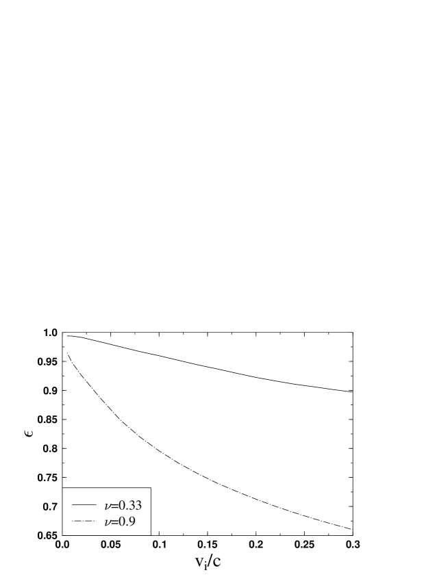
FIG. 1.:

FIG. 2.:

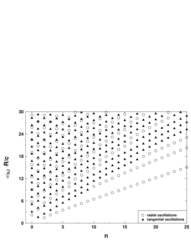
FIG. 3.:

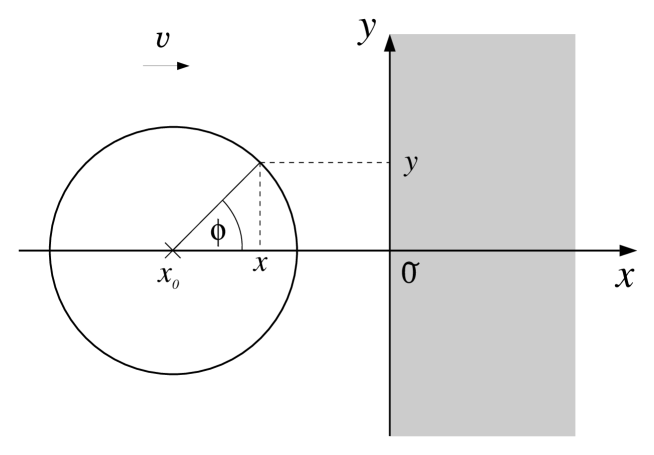
FIG. 4.:

FIG. 5.:

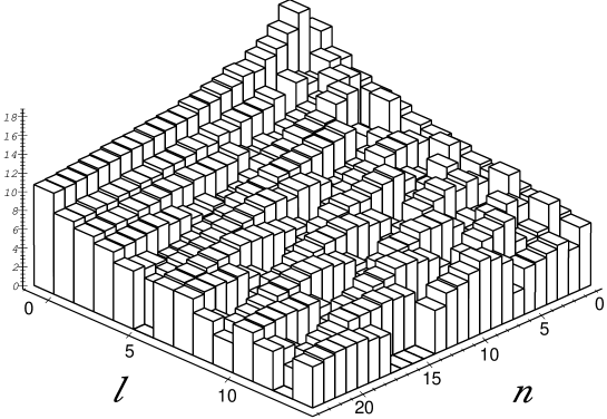
FIG. 6.:

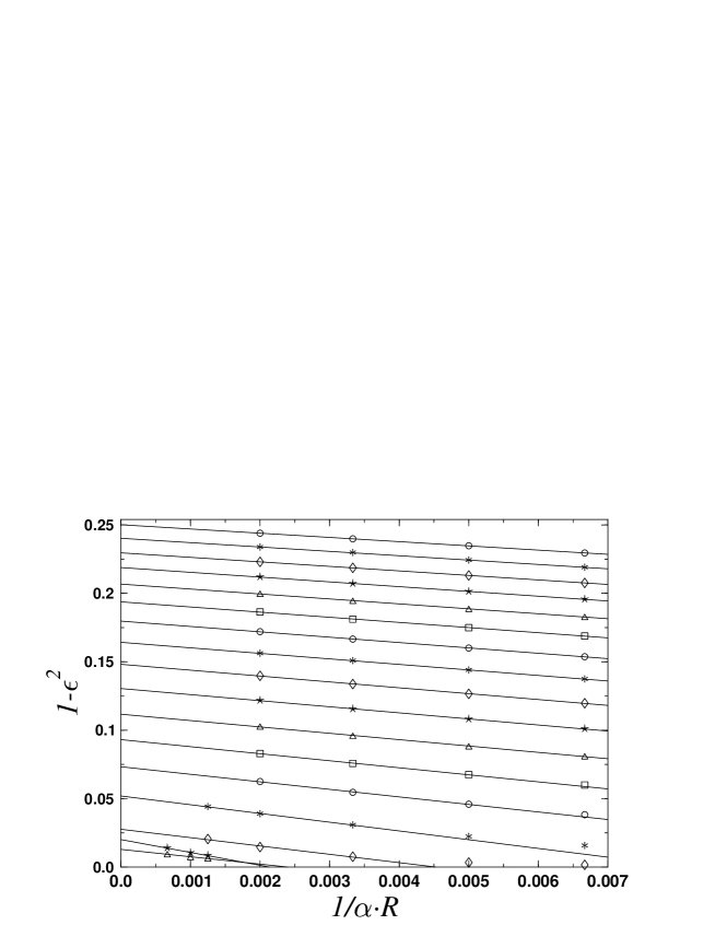
FIG. 7.:

FIG. 8.:

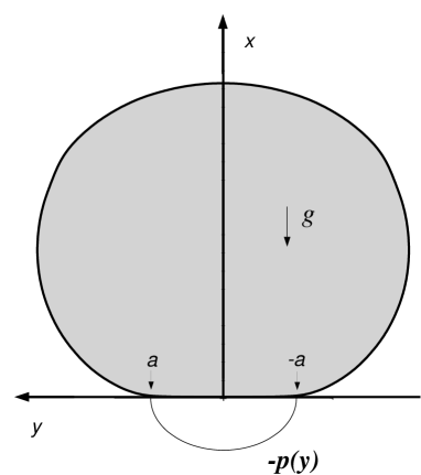
FIG. 9.:

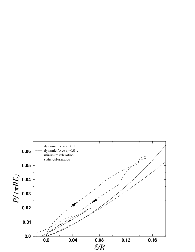
FIG. 10.:

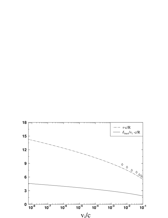
FIG. 11.:

FIG. 12.:

REFERENCES

- [1] See, for example, B. Bernu and M. Mazighi, J. Phys. A23, 5745 (1990); B. Bernu, F. Delyon, and R. Mazighi, Phys. Rev E50, 4551 (1994); B. D. Lubachevsky, J. Comp. Phys. 94, 255 (1991); S. McNamara and W. R. Young, Phys. Fluids A4, 496 (1992); ibid 5, 34 (1993); E. Clément, S. Luding, A. Blumen, J. Rajchenbach and J. Duran, Intern. J. Mod. Phys. B7, 1807 (1993); S. McNamara and W. R. Young, Phys. Rev. E, 50, R28 (1994);
- [2] A. P. Hatzes, F. G. Bridges, and D. N. C. Lin, Mon. Not. R. Astron. Soc. 231 1091 (1988); K. D. Supulver, Fg G. Bridges, and D. N. C. Lin, Icarus 113, 188 (1995).
- [3] See, for example, J.A.C. Gallas, H.J. Herrmann, and S. Sokolowski, Phys. Rev. Lett. 69, 1371 (1992); Physica A189, 437 (1992); Y-h. Taguchi, Phys. Rev. Lett. 69, 1367 (1992); J. Phys. (Paris) II 2, 2103 (1992); Int. J. Mod. Phys. B7, 1839 (1993); T. Poeschel, J. Phys. (Paris) II 3, 27 (1993); J. A. C. Gallas et al., J. Stat. Phys. 82, 443 (1996); S. Luding, E. Clément, A. Blumen, J. Rajchenbach, and J. Duran, Phys. Rev. E 50, 4113 (1994)
- [4] D. E. Wolf, Modeling and Computer Simulations of Granular media , in Computational Physics, K.H. Hoffmann and M. Schreiber (Eds.), Berlin (1996), p.64 (Springer).
- [5] D. Tabor, Proc. Roy. Soc A172, 247 (1948); J. P. Andrews, Phil.Mag. Series 7 9, 593 (1939)
- [6] H. Hertz, J. Reine und Angewandte Math. 92, 156-71 (1882)
- [7] T. Pöschel, Z. Phys. 46, 142 (1928), J. P. Dilley, Icarus 105, 225 (1993)
- [8] N. V. Brilliantov, F. Spahn, J-M. Hertzsch and T. Pöschel, Phys. Rev. E 53 5382 (1996)
- [9] G. Giese and A. Zippelius, Phys. Rev. E 54, 4828 (1996)
- [10] T. Aspelmeier, G. Giese and A. Zippelius, Phys. Rev. E57, 857 (1998).
- [11] T. Aspelmeier and A. Zippelius, preprint
- [12] O. M. Rayleigh, Phil. Mag. Series 6 11, 283 (1906)
- [13] A. E. H. Love, A Treatise on the Mathematical Theory of Elasicity 4th ed., Cambridge University Press, Cambridge, 1952, p.497
- [14] L. D. Landau and E. M. Lifschitz, Lehrbuch der Theoretischen Physik, Band VII Elastizitätstheorie, Akademie Verlag, Berlin, 1965
- [15] S. Timoshenko and J. N. Goodier, Theory of Elasticity, 3rd ed. McGraw Hill, New York 1951
- [16] M. Abramowitz and I. Stegun,Handbook of Mathematical Functions, Dover Publicatons, New York, 1965
- [17] J. H. Michell, Proc. Lond. Math. Soc. 32 , 44 (1900)
- [18] K. L. Johnson, Contact Mechanics, Cambridge University Press, Cambridge, 1985, chapter 4.2 pp. 99
- [19] K. L. Johnson, loc. cit. chapter 5.6