Unified View of Scaling Laws for River Networks
Phys. Rev. E 59(5), May 1999

Abstract

Scaling laws that describe the structure of river networks are shown to follow from three simple assumptions. These assumptions are: (1) river networks are structurally self-similar, (2) single channels are self-affine, and (3) overland flow into channels occurs over a characteristic distance (drainage density is uniform). We obtain a complete set of scaling relations connecting the exponents of these scaling laws and find that only two of these exponents are independent. We further demonstrate that the two predominant descriptions of network structure (Tokunaga’s law and Horton’s laws) are equivalent in the case of landscapes with uniform drainage density. The results are tested with data from both real landscapes and a special class of random networks.

I Introduction

If it is true that scaling laws abound in nature mandelbrot83 , then river networks stand as a superb epitome of this phenomenon. For over half a century, researchers have uncovered numerous power laws and scaling behaviors in the mathematical description of river networks horton45 ; langbein47 ; strahler52 ; hack57 ; tarboton88 ; labarbera89 ; tarboton90 ; maritan96a . These scaling laws, which are usually parameterized by exponents or ratios of fundamental quantities, have been used to validate scores of numerical and theoretical models of landscape evolution leopold62 ; shreve66 ; howard71b ; stark91 ; meakin91 ; willgoose91a ; willgoose91c ; willgoose91 ; kramer92 ; leheny93 ; sun94 ; sun94b ; somfai97 ; rodriguez-iturbe97 and have even been invoked as evidence of self-organized criticality rodriguez-iturbe97 ; bak97 . However, despite this widespread usage, there is as yet no fundamental understanding of the origin of scaling laws in river networks.

It is the principal aim of this paper to bring together a large family of these scaling laws within a simple, logical framework. In particular, we demonstrate that from a base of three assumptions regarding network geometry, all scaling laws involving planform quantities may be obtained. The worth of these consequent scaling laws is then seen to rest squarely upon the shoulders of the structural assumptions themselves. We also simplify the relations between the derived laws, demonstrating that only two scaling exponents are independent.

The paper is composed in the following manner. We first present preliminary definitions of network quantities and a list of empirically observed scaling laws. Our assumptions will next be fully stated along with evidence for their validity. Several sections will then detail the derivations of the various scaling laws, being a combination of both new insights of our own as well as previous results. Progressing in a systematic way from our assumptions, we will also be required to amend several inconsistencies persistent in other analyses. The theory will be tested with comparisons to data taken from real landscapes and Scheidegger’s random network model scheidegger67b ; scheidegger90 .

II The ordering of streams

A basic tool used in the analysis of river networks is the device of stream ordering. A stream ordering is any scheme that attaches levels of significance to streams throughout a basin. Most orderings identify the smallest tributaries as lowest order streams and the main or ‘trunk’ stream as being of highest order with the intermediary ‘stream segments’ spanning this range in some systematic fashion. Stream orderings allow for logical comparisons between different parts of a network and provide a basic language for the description of network structure.

Here, we build our theory using the most common ordering scheme, one that was first introduced by Horton in his seminal work on erosion horton45 . Strahler later improved this method strahler57 and the resulting technique is commonly referred to as Horton-Strahler stream ordering rodriguez-iturbe97 . The most natural description of this stream ordering, due to Melton melton59 , is based on an iterative pruning of a tree representing a network as shown in Figure 1. All source (or external) streams are pared away from the tree, these being defined as the network’s first order ‘stream segments’. A new tree is thus created along with a new collection of source streams and these are precisely the second order stream segments of the original network. The pruning and order identification continues in like fashion until only the trunk stream segment of the river network is left. The overall order of the basin itself is identified with the highest stream order present.

The usual and equivalent description details how stream orders change at junctions rodriguez-iturbe97 . When a stream segment of order $\omega_{1}$ merges with a stream segment of order $\omega_{2}$, the outgoing stream will have an order of $\omega$ given by

$$\omega=\max(\omega_{1},\omega_{2})+\delta_{\omega_{1},\omega_{2}}$$ (1)

where $\delta$ is the Kronecker delta. In other words, stream order only increases when two stream segments of the same order come together and, otherwise, the highest order is maintained by the outflowing stream.

Figure 1: Horton-Strahler stream ordering. (a) shows the basic network. (b) is created by removing all source streams from the network in (a), these same streams being denoted as first order ‘stream segments’. The new source streams in the pruned network of (b) are labelled as second order stream segments and are themselves removed to give (c), a third order stream segment.

III Planform network quantities and scaling laws

The results of this paper pertain to networks as viewed in planform. As such, any effects involving relief, the vertical dimension, are ignored. Nevertheless, we show that a coherent theory of planform quantities may still be obtained. This section defines the relevant quantities and their various permutations along with scaling laws observed to hold between them. The descriptions of these laws will be short and more detail will be provided in later sections.

The two essential features in river networks are basins and the streams that drain them. The two basic planform quantities associated with these are drainage area and stream length. An understanding of the distribution of these quantities is of fundamental importance in geomorphology. Drainage area, for example, serves as a measure of average discharge of a basin while its relationship with the length of the main stream gives a sense of how basins are shaped.

III.1 General network quantities

Figure 2 shows a typical drainage basin. The basin features are $a$, the area, $l$, the length of the main stream, and $L_{\parallel}$ and $L_{\perp}$, the overall dimensions. The main (or trunk) stream is the dominant stream of the network—it is traced out by moving all the way upstream from the outlet to the start of a source stream by choosing at each junction (or fork) the incoming stream with the largest drainage area. This is not to be confused with stream segment length which only makes sense in the context of stream ordering. We will usually write $L$ for $L_{\parallel}$. Note that any point on a network has its own basin and associated main stream. The sub-basin in Figure 2 illustrates this and has its own primed versions of $a$, $l$, $L_{\parallel}$ and $L_{\perp}$. The scaling laws usually involve comparisons between basins of varying size. These basins must be from the same landscape and may or may not be contained within each other.

Several scaling laws connect these quantities. One of the most well known is Hack’s law hack57 . Hack’s law states that $l$ scales with $a$ as

$$l\sim a^{h}$$ (2)

where $h$ is often referred to as Hack’s exponent. The important feature of Hack’s law is that $h\neq 1/2$. In particular, it has been observed that for a reasonable span of basin sizes that $0.57<h<0.60$ hack57 ; maritan96a ; gray61 ; rigon96 . The actual range of this scaling is an unresolved issue with some studies demonstrating that very large basins exhibit the more expected scaling of $h=1/2$ mueller72 ; mosley73 ; mueller73 . We simply show later that while the assumptions of this paper hold so too does Hack’s law.

Further comparisons of drainage basins of different sizes yield scaling in terms of $L(=L_{\parallel})$, the overall basin length. Area, main stream length, and basin width are all observed to scale with $L$ maritan96a ; tarboton88 ; labarbera89 ; tarboton90 ; labarbera90 ,

$$a\sim L^{D},\qquad l\sim L^{{d}},\qquad L_{\perp}\sim L^{H}.$$ (3)

Turning our attention to the entire landscape, it is also observed that histograms of stream lengths and basin areas reveal power law distributions maritan96a ; rodriguez-iturbe97 :

$$P(a)\sim a^{-\tau}\qquad\mbox{and}\qquad P(l)\sim l^{-\gamma}.$$ (4)

There are any number of other definable quantities and we will limit ourselves to a few that are closely related to each other. We write $\lambda$ for the average distance from a point on the network to the outlet of a basin (along streams) and $\Lambda$ for the unnormalized total of these distances. A minor variation of these are $\tilde{\lambda}$ and $\tilde{\Lambda}$, where only distances from junctions in the network to the outlet are included in the averages.

The scaling law involving these particular quantities is Langbein’s law langbein47 which states that

$$\Lambda\sim a^{\beta}.$$ (5)

Similarly, we have $\lambda\sim L^{\varphi}$, $\tilde{\Lambda}\sim a^{\tilde{\beta}}$ and $\tilde{\lambda}\sim L^{\tilde{\varphi}}$, maritan96a .

Figure 2: A planform view of an example basin. The main defining parameters of a basin are $a$, the drainage area, $l$, the length of the main stream, and $L_{\parallel}$ and $L_{\perp}$, the overall Euclidean dimensions. The sub-basin with primed quantities demonstrates that a basin exists at every point in a network.

III.2 Network quantities associated with stream ordering

With the introduction of stream ordering, a whole new collection of network quantities appear. Here, we present the most important ones and discuss them in the context of what we identify as the principal structural laws of river networks: Tokunaga’s law and Horton’s laws.

III.2.1 Tokunaga’s law

Tokunaga’s law concerns the set of ratios, $\{T_{\omega,\omega^{\prime}}\}$, first introduced by Tokunaga tokunaga66 ; tokunaga78 ; tokunaga84 ; peckham95 ; newman97 . These ‘Tokunaga ratios’ represent the average number of streams of order $\omega^{\prime}$ flowing into a stream of order $\omega$ as side tributaries. In the case of what we will call a ‘structurally self-similar network’, we have that $T_{\omega,\omega^{\prime}}=T_{\omega-\omega^{\prime}}=T_{\nu}$ where $\nu=\omega-\omega^{\prime}$ since quantities involving comparisons between features at different scales should only depend on the relative separation of those scales. These $T_{\nu}$, in turn, are observed to be dependent such that tokunaga66 ,

$$T_{\nu+1}/T_{\nu}=R_{T}$$ (6)

where $R_{T}$ is a fixed constant for a given network. Thus, all of Tokunaga’s ratios may be specified by two fundamental parameters $T_{1}$ and $R_{T}$:

$$T_{\nu}=T_{1}(R_{T})^{\nu-1}.$$ (7)

We refer to this last identity as Tokunaga’s law.

The network parameter $T_{1}$ is the average number of major side tributaries per stream segment. So for a collection of stream segments of order $\omega$, there will be on average $T_{1}$ side tributaries of order $\omega-1$ for each stream segment. The second network parameter $R_{T}$ describes how numbers of side tributaries of successively lower orders increase, again, on average. As an example, consider that the network in Figure 1 is part of a much larger network for which $T_{1}=2$ and $R_{T}=4$. Figure 1 (b) shows that the third order stream segment has two major side tributaries of second order which fits exactly with $T_{1}=2$ (Note that the two second order stream segments that come together to create the third order stream segment are not side tributaries). Figure 1 (a) further shows nine first order tributaries, slightly above the average eight suggested by $T_{2}=T_{1}R_{T}^{1}=8$. Finally, again referring to Figure 1 (a), there are $9/4=2.25$ first order tributaries for each second order stream segment, not far from the expected number $T_{1}=2$.

III.2.2 Horton’s laws

Horton introduced several important measurements for networks in conjunction with his stream ordering horton45 . The first is the bifurcation ratio, $R_{n}$. This is the ratio of the number $n_{\omega}$ of streams of order $\omega$ to the number $n_{\omega+1}$ of streams of order $\omega+1$ and is, moreover, observed to be independent of $\omega$ over a large range. There is next the stream length ratio, $R_{\ell}=\bar{\ell}_{\omega+1}/\bar{\ell}_{\omega}$, where $\bar{\ell}_{\omega}$ is the average length of stream segments of order $\omega$. These lengths only exist within the context of stream ordering. In contrast to these are the main stream lengths, which we have denoted by $l$ and described in section III.1. Main stream lengths are defined regardless of stream ordering and, as such, are a more natural quantity. Note that stream ordering gives rise to a discrete set of basins, one for each junction in the network. We therefore also have a set of basin areas and main stream lengths defined at each junction. Taking averages over basins of the same order we have $\bar{a}_{\omega}$ and $\bar{l}_{\omega}$ to add to the previously defined $\bar{\ell}_{\omega}$ and $n_{\omega}$.

The connection between the two measures of stream length is an important, if simple, exercise scheidegger68c . Assuming $\bar{\ell}_{\omega+1}=R_{\ell}\bar{\ell}_{\omega}$ holds for all $\omega$, one has

$$\bar{l}_{\omega}=\sum_{i=1}^{\omega}\bar{\ell}_{i}=\sum_{i=1}^{\omega}(R_{\ell})^{i-1}\bar{\ell}_{1}=\bar{l}_{1}\frac{(R_{\ell})^{\omega}-1}{R_{\ell}-1}$$ (8)

where $\bar{l}_{1}=\bar{\ell}_{1}$ has been used. Since typically $R_{\ell}>2$ kirchner93 , $\bar{l}_{\omega+1}/\bar{l}_{\omega}\rightarrow R_{\ell}$ rapidly. For $\omega=4$ and $R_{\ell}=2$, the error is only three per cent. On the other hand, starting with the assumption that main stream lengths satisfy Horton’s law of stream lengths for all $\omega$ implies that the same is true for stream segments.

Thus, for most calculations, Horton’s law of stream lengths may involve either stream segments or main streams and, for convenience, we will assume that the law is fully satisfied by the former. Furthermore, this small calculation suggests that studies involving only third- or fourth-order networks cannot be presumed to have reached asymptotic regimes of scaling laws. We will return to this point throughout the paper.

Schumm schumm56a is attributed with the concrete introduction of a third and final law that was also suggested by Horton. This last ratio is for drainage areas and states that $R_{a}=\bar{a}_{\omega+1}/\bar{a}_{\omega}$. We will later show in section VII that our assumptions lead to the result that $R_{a}\equiv R_{n}$. At this stage, however, we write Horton’s laws as the three statements

$$\frac{n_{\omega}}{n_{\omega+1}}=R_{n},\ \frac{\bar{\ell}_{\omega+1}}{\bar{\ell}_{\omega}}=R_{\ell},\ \mbox{and}\ \frac{\bar{a}_{\omega+1}}{\bar{a}_{\omega}}=R_{a}.$$ (9)

A summary of all of the scaling laws presented in this section is provided in Table 1. Empirically observed values for the relevant exponents and ratios are presented in Table 2.

Law:	Name or description:
$T_{\nu}=T_{1}(R_{T})^{\nu-1}$	Tokunaga’s law
$l\sim L^{{d}}$	self-affinity of single channels
$n_{\omega+1}/n_{\omega}=R_{n}$	Horton’s law of stream numbers
$\bar{\ell}_{\omega+1}/\bar{\ell}_{\omega}=R_{\ell}$	Horton’s law of stream segment lengths
$\bar{l}_{\omega+1}/\bar{l}_{\omega}=R_{\ell}$	Horton’s law of main stream lengths
$\bar{a}_{\omega+1}/\bar{a}_{\omega}=R_{a}$	Horton’s law of stream areas
$l\sim a^{h}$	Hack’s law
$a\sim L^{D}$	scaling of basin areas
$L_{\perp}\sim L^{H}$	scaling of basin widths
$P(a)\sim a^{-\tau}$	probability of basin areas
$P(l)\sim l^{-\gamma}$	probability of stream lengths
$\Lambda\sim a^{\beta}$	Langbein’s law
$\lambda\sim L^{\varphi}$	variation of Langbein’s law
$\tilde{\Lambda}\sim a^{\tilde{\beta}}$	as above
$\tilde{\lambda}\sim L^{\tilde{\varphi}}$	as above

Table 1: A general list of scaling laws for river networks. All laws and quantities are defined in section III. The principal finding of this paper is that these scaling laws follow from the first two relations, Tokunaga’s law (structural self-similarity) and the self-affinity of single channels, and the assumption of uniform drainage density (defined in section IV.3).

III.3 Scheidegger’s random networks

To end this introductory section, we detail some of the features of the random network model of Scheidegger scheidegger67b ; scheidegger90 . Although originally defined without reference to a real surface, Scheidegger networks may be obtained from a completely uncorrelated landscape as follows. Assign a random height between 0 and 1 at every point on a triangular lattice and then tilt the lattice so that no local minima (lakes) remain. Scheidegger networks are then traced out by following paths of steepest descent.

Surprisingly, these networks still exhibit all of the scaling laws observed in real networks. It thus provides an important point in ‘network space’ and accordingly, also provides an elementary test for any theory of scaling laws. Exact analytical results for various exponents are known due to the work of Takayasu et al. on the aggregation of particles with injection takayasu88 ; takayasu89a ; takayasu89b ; takayasu90 ; takayasu91 ; huber91 . While there are no analytic results for the Tokunaga ratio $T_{1}$ or the Horton ratios $R_{n}$ and $R_{\ell}$, our own simulations show that these stream order laws are strictly obeyed. Table 2 lists the relevant exponents and their values for the Scheidegger model along with those found in real networks.

Quantity:	Scheidegger:	Real networks:
$R_{n}$	$5.20\pm.05$	3.0–5.0 abrahams84
$R_{a}$	$5.20\pm.05$	3.0–6.0 abrahams84
$R_{\ell}$	$3.00\pm.05$	1.5–3.0 abrahams84
$T_{1}$	$1.30\pm.05$	1.0–1.5 tokunaga78
${d}$	$1$	$1.1\pm 0.01$ maritan96a
$D$	$3/2$	$1.8\pm 0.1$ maritan96a
$h$	$2/3$	0.57–0.60 maritan96a
$\tau$	$4/3$	$1.43\pm 0.02$ maritan96a
$\gamma$	$3/2$	$1.8\pm 0.1$ rigon96
$\varphi$	$1$	$1.05\pm 0.01$ maritan96a
$H$	$1/2$	0.75–0.80 maritan96a
$\beta$	$5/3$	1.56 langbein47
$\varphi$	$1$	$1.05\pm 0.01$ maritan96a

Table 2: Ratios and scaling exponents for Scheidegger’s random network model and real networks. For Scheidegger’s model, exact values are known due to the work of Takayasu et al. takayasu88 ; takayasu89a ; takayasu89b ; takayasu90 ; takayasu91 ; huber91 and approximate results are taken from our own simulations. For real networks, the references given are generally the most recent and further appropriate references may be found within them and also in section III.

IV Assumptions

We start from three basic assumptions about the structure of river networks: structural self-similarity, self-affinity of individual streams and uniformity of drainage density. We define these assumptions and their relevant parameters and then discuss their mutual consistency. We end with a discussion of the correspondence between the laws of Tokunaga and Horton. It should be stressed that while we make a case for each assumption there is also considerable proof to ponder in the pudding that these ingredients create.

IV.1 Structural self-similarity

Our first assumption is that networks are structurally self-similar. It has been observed that river networks exhibit self-similarity over a large range of scales mandelbrot83 ; tarboton88 ; rodriguez-iturbe97 . Naturally, the physical range of this self-similarity is restricted to lie between two scales. The large scale cutoff is the overall size of the landscape and the small scale cutoff is of the order of the characteristic separation of channels montgomery92 .

In order to quantify this phenomenon, we look to laws of network structure such as Tokunaga’s law and Horton’s laws of stream number and length. We demonstrate in the following section that these descriptions are mutually consistent within the context of our third assumption, uniformity of drainage density. Thus, we may assume a network where both Tokunaga’s and Horton’s laws hold. For convenience, we write these laws as if they hold for all orders down to the first order. Any actual deviations from these laws for low orders will not affect the results since we are interested in how laws behave for increasing stream order.

IV.2 Self-affinity of individual streams

Our second assumption is that individual streams are self-affine curves possessing a dimension ${d}>1$, as introduced in equation (3). Empirical support for this premise is to be found in tarboton88 ; labarbera89 ; tarboton90 ; maritan96a ; rodriguez-iturbe97 ; tarboton89 . In reality, this is at best a weak fractality with measurements generally finding ${d}$ to be around $1.1$ maritan96a . We assume ${d}$ to be constant throughout a given network, true for each stream independent of order.

In general, it is most reasonable to consider this in the sense of a growing fractal: stream length $l$ will grow like $L^{{d}}$ where $L$ is the overall length of a box containing a portion of a stream. So, rather than examine one fixed section of a stream, we take larger and larger pieces of it. Moreover, this is the most reasonable method for actually measuring ${d}$ for a real network.

IV.3 Uniform drainage density

Our third and final assumption is that drainage density is uniform throughout a network. For a given basin, the drainage density, $\rho$, is a measure of the average area drained per unit length of stream by overland flow (i.e., excluding contributions from tributary streams). Its usual form is that given by Horton horton45 :

$$\rho=\frac{\sum\ell}{a}$$ (10)

where, for a given basin, $\sum\ell$ represents the summed total length of all stream segments of all orders and $a$ is the drainage area. More generally, one can in the same way measure a local drainage density for any connected sections of a network within a landscape. Such sections should cover a region at least $\ell_{1}$ in diameter, the typical length of a first order stream. Drainage density being uniform means that the variation of this local drainage density is negligible. There is good support in the literature for the uniformity of drainage density in real networks hack57 ; shreve67 ; haggett69 ; gardiner73 ; morisawa62 ; devries94 while there are some suggestions that it may vary slightly with order hack57 ; tokunaga78 .

Uniform drainage density may also be interpreted as the observation that the average distance between channels is roughly constant throughout a landscape horton45 ; rodriguez-iturbe97 , an estimate of this distance being simply $1/\rho$. This is due to the fact that there is a finite limit to the channelization of a landscape determined by a combination of soil properties, climate and so on. Implicit in this assumption is that the channel network has reached its maximum extension into a landscape shreve67 ; glock31 . Indeed, In the bold words of Glock glock31 , we are considering river networks at the “time of completed territorial conquest.” Furthermore, Shreve shreve67 notes that drainage density would be uniform in a “mature topography developed in a homogeneous environment.”

Importantly, our third assumption connects the planform description to the surface within which the network lies. Computationally, the uniformity of drainage density allows for the use of the length of a stream as a proxy for drainage area devries94 . Further, the average distance between streams being roughly constant implies that, on average, tributaries are spaced evenly along a stream.

V Tokunaga’s law and Horton’s laws are equivalent

This section demonstrates an equivalence between Tokunaga’s law and Horton’s two laws of stream number and stream length in the case of a landscape with uniform drainage density.

V.1 From Tokunaga’s law to Horton’s laws

Tokunaga has shown that Horton’s law for stream numbers follows from Tokunaga’s law (given in equation (7)) tokunaga78 ; peckham95 . This follows from the observation that $n_{\omega}$, the number of streams of order $\omega$, in a basin of order $\Omega$ may be expressed as

$$n_{\omega}=2n_{\omega+1}+\sum_{\nu=1}^{\Omega-\omega}T_{\nu}n_{\omega+\nu}.$$ (11)

The $2n_{\omega+1}$ accounts for the fact that each order $\omega+1$ stream is initiated by the confluence of two streams of order $\omega$. Presuming Tokunaga’s law, a simple analysis of equation (11) shows that in the limit of large $\Omega$, the ratio $n_{\omega}/n_{\omega+1}$ does indeed approach a constant. This leads to an expression for the Horton ratio $R_{n}$ in terms of the two Tokunaga parameters $T_{1}$ and $R_{T}$ (first obtained by Tokunaga in tokunaga78 ):

$$2R_{n}=(2+R_{T}+T_{1})+\left[(2+R_{T}+T_{1})^{2}-8R_{T}\right]^{1/2}.$$ (12)

Tokunaga’s work has been recently generalized by Peckham who deduces links to the other Horton ratios $R_{\ell}$ and $R_{a}$ peckham95 . In contrast to the purely algebraic calculation of $R_{n}$, these results require the step of equating topological properties to metric basin quantities. In determining $R_{\ell}$, Peckham uses the number of side tributaries to a stream as an estimate of stream segment length. This is based on the assumption that tributaries are evenly spaced. As discussed in section IV.3, this even spacing of tributaries follows for networks with uniform drainage density. Therefore, we may write, after Peckham, that

$$\bar{\ell}_{\omega}\propto 1+\sum_{\nu=1}^{\omega-1}{T_{\nu}}$$ (13)

where the dimension of length absent on the right-hand side is carried by an appropriate constant of proportionality. This sum is simply the total number of tributaries that, on average, enter a stream of order $\omega$. The number of lengths of stream between tributaries is then simply one more in number.

Using Tokunaga’s law (equation (7)) we find that

$$\bar{\ell}_{\omega+1}/\bar{\ell}_{\omega}=R_{T}\left(1+O(R_{T})^{-\omega}\right),$$ (14)

obtaining Horton’s stream length ratio with the simple identification:

$$R_{\ell}=R_{T}$$ (15)

and we will use $R_{\ell}$ in place of $R_{T}$ throughout the rest of the paper. As already noted we will see that $R_{a}\equiv R_{n}$ for landscapes where drainage density is uniform. This redundancy means that there are only two independent Horton ratios, $R_{\ell}$ and $R_{n}$, which sits well with the two independent quantities required for Tokunaga’s law, $T_{1}$ and $R_{T}$. Presupposing this result, we can invert equations (12) and (15) to obtain Tokunaga’s parameters from the two independent Horton ratios:

$$R_{T} = R_{\ell}$$ (16)

$$T_{1} = R_{n}-R_{\ell}-2+2R_{\ell}/R_{n}.$$ (17)

V.2 From Horton’s laws to Tokunaga’s law

We now provide an heuristic argument to show that Tokunaga’s law in the form of equation (7) follows from Horton’s laws of stream number and length and uniform drainage density. Note that even though we have shown in equations (12), (15), and (17) that the parameters of Tokunaga’s law and those of Horton’s laws may be obtained from each other, it is not a priori clear that this result would be true. Indeed, Tokunaga’s law contains more direct information about network structure than Horton’s laws and it is the additional constraint of uniform drainage density that provides the key.

Consider a stream of order $\omega$ along with its side tributaries of order $\omega^{\prime}=1$ through $\omega^{\prime}=\omega-1$, the numbers of which are given by the usual $T_{\nu}$ where $\nu=\omega-\omega^{\prime}$ (see Figure 3). Since the presumed adherence to Horton’s laws implies that a network is self-similar we need only consider the form of the $T_{\nu}$ and not the more general $T_{\omega^{\prime},\omega}$. Now, again since networks are self-similar, a typical stream of order $\omega+1$ can be obtained by scaling up the picture of this order $\omega$ stream. As per Horton’s law of stream lengths, this is done by increasing the length of each stream by a factor of $R_{\ell}$ (Figure 3 (a) becomes Figure 3 (b)).

However, since order $\omega^{\prime}$ streams become $\omega^{\prime}+1$ streams in this rescaling, the picture in Figure 3 (b) is missing first order streams. Also, the average distance between tributaries has grown by a factor of $R_{\ell}$. Therefore, to retain the same drainage density, an extra $(R_{\ell}-1)$ first order streams must be added for each link (one more than the number of tributaries) along this new order $\omega+1$ stream (Figure 3 (c)). Since the number of first order streams is now given by $T_{\omega+1}$ we have

$$T_{\omega+1}=(R_{\ell}-1)\left(\sum_{\nu=1}^{\omega}T_{\nu}+1\right).$$ (18)

It may be simply checked that this equation is satisfied, for large $\omega$, by Tokunaga ratios given by equation (7). Thus, Horton’s laws of stream number and stream length and the uniform drainage density are seen to imply Tokunaga’s law.

Figure 3: An example rescaling of a basin to demonstrate how Tokunaga’s law follows from Horton’s laws and uniform drainage density. In the first step from (a) to (b), the streams of the small network are rescaled in length by a factor of $R_{\ell}$. The second step from (b) to (c) demonstrates that for drainage density to remain constant and uniform, a sufficient number of first order tributaries must be added.

In general, Horton’s ratios rather than the parameters of Tokunaga’s law will be the most useful parameters in what follows. In particular, we will see that the two independent quantities $R_{n}$ and $R_{\ell}$ will be needed only in the form $\ln R_{n}/\ln R_{\ell}$. All other exponents will be expressible as algebraic combinations of $\ln R_{n}/\ln R_{\ell}$ and ${d}$, the fractal dimension of an individual stream.

Furthermore, example (or modal) values for the parameters of Horton and Tokunaga are tokunaga78 ; kirchner93

$$T_{1}=1,\ R_{T}=R_{\ell}=2,\ \mbox{and}\ R_{n}=4.$$ (19)

The parameters have been chosen so as to satisfy the inversion relations of equation (17). As shown in Table 2, real networks provide some variation around these modal values. These will be used as rough checks of accuracy throughout the rest of the paper.

VI Hack’s law

One of the most intriguing scalings found in river networks is Hack’s law hack57 which relates main stream length to basin area as $l\sim a^{h}$. This equation has been empirically shown to hold true for a large range of drainage basin sizes on many field sites rodriguez-iturbe97 . The salient feature is that for smaller basins rigon96 , $h$ is typically found to be in the range $(0.56,0.60)$, whereas $0.5$ would be expected from simple dimensional analysis rodriguez-iturbe97 .

It should be emphasized that Hack’s law is only true on average as are, for that matter, Tokunaga’s law and Horton’s laws. An extension of Hack’s law to a more natural statistical description of the connection between stream lengths and drainage areas was suggested by Maritan et al. maritan96a with some further developments to be found in dodds98d .

VI.1 Horton’s other law of stream numbers

In order to obtain Hack’s law, we will use the uniformity of drainage density to estimate the area of an order $\Omega$ basin by calculating the total length of streams within the same basin. So we simply need the typical length and number of each stream order present. Taking the length of a source stream, $\bar{\ell}_{1}$, to be the finest resolution of the network and the basic unit of length, the length of a stream segment of order $\omega$ is $\bar{\ell}_{\omega}=(R_{\ell})^{\omega-1}\bar{\ell}_{1}$. However, in finding the frequency of such streams we find that some care must be taken for the following reasons.

Horton’s law of stream numbers is potentially misleading in that it suggests, at first glance, that within a basin of order $\omega$ there should be one stream of order $\omega$, $R_{n}$ streams of order $\omega-1$, $R_{n}^{2}$ streams of order $\omega-2$ and so on. Indeed, many calculations involving Horton’s laws use this assumption labarbera89 ; rodriguez-iturbe97 ; devries94 ; rosso91 .

But Horton’s $R_{n}$ actually provides the ratio of the number of streams of consecutive orders as totalled for a whole basin. To illustrate this fact, consider streams of order $\omega$ and $\omega+1$ within a basin of order $\Omega\gg\omega$. As Tokunaga’s law makes clear, streams of order $\omega$ are not all found within sub-basins of order $\omega+1$. Indeed, a certain number of order $\omega$ streams will be tributaries to streams of order greater than $\omega+1$ (see the example network of Figure 1 (a)). Tokunaga’s law shows that we should in fact expect $T_{1}+2$ rather than than $R_{n}$ streams of order $\omega$ entering into a stream of order $\omega+1$. For the typical values $T_{1}=1$ and $R_{n}=4$ in (19) this is a substantial error.

We proceed then to find a corrected version of Horton’s law of stream numbers. Returning to equation (11), we see that it is only valid in the limit $\Omega\rightarrow\infty$. Defining $n^{\prime}(\omega,\Omega)$ as the actual number of streams of order $\omega$ within a basin of order $\Omega$, we have

$$n^{\prime}(\omega,\Omega)=2n^{\prime}(\omega+1,\Omega)+\sum_{\nu=1}^{\Omega-\omega}T_{\nu}n^{\prime}(\omega+\nu,\Omega).$$ (20)

This equation may be exactly solved. Considering the above expression for $n^{\prime}(\omega,\Omega)$ and the corresponding one for $n^{\prime}(\omega+1,\Omega)$ we can reduce this to a simple difference equation,

$$n^{\prime}(\omega,\Omega)=(2+R_{\ell}+T_{1})n^{\prime}(\omega+1,\Omega)-2R_{\ell}n^{\prime}(\omega+2,\Omega)$$ (21)

which has solutions of the form $\mu^{k}$. Applying the constraints that $n^{\prime}(\Omega,\Omega)=1$ and $n^{\prime}(\Omega-1,\Omega)=T_{1}+2$, we obtain

$$n^{\prime}(\omega,\Omega)=c(\mu_{+})^{\Omega-\omega}+(1-c)(\mu_{-})^{\Omega-\omega}$$ (22)

where

$$2\mu_{\pm}=(2+R_{\ell}+T_{1})\pm\left[(2+R_{\ell}+T_{1})^{2}-8R_{\ell}\right]^{1/2}$$ (23)

and

$$c=R_{n}(R_{n}-R_{\ell})/(R_{n}^{2}-2R_{\ell}).$$ (24)

Note that $R_{n}=\mu_{+}$ and we will use the notation $R_{n}^{\ast}$ in place of $\mu_{-}$. This observation regarding Horton’s law of stream numbers was first made by Tokunaga tokunaga66 and later by Smart smart67 . In particular, Tokunaga noted that this would explain the deviation of Horton’s law for the highest orders of a basin, a strong motivation for his work.

We can now define an effective Horton ratio, ${R_{n}}^{\prime}(\omega,\Omega)$ as follows:

$${R_{n}}^{\prime}(\omega,\Omega) = n^{\prime}(\omega-1,\Omega)/n^{\prime}(\omega,\Omega)$$ (25)

$$= R_{n}\left(1+O(R_{n}^{\ast}/R_{n})^{(\Omega-\omega)}\right)$$

The typical values of Horton’s ratios in (19) give $R_{n}^{\ast}=1$. In this case, ${R_{n}}^{\prime}(\omega,\Omega)$ converges rapidly to $R_{n}$ with an error of around one per cent for $\omega=\Omega-3$.

VI.2 Hack’s law

As discussed in section IV.3, an estimate of total drainage area of a basin is given by the total length of all streams within the basin. Summing over all stream orders and using the numbers $n^{\prime}(\omega,\Omega)$ given by equations (22) and (23) we have that

$$\bar{a}_{\Omega} \propto \sum_{\omega=1}^{\Omega}n^{\prime}(\omega,\Omega)(R_{\ell})^{\omega-1}$$ (26)

$$= c_{1}(R_{n})^{\Omega}+c_{2}(R_{\ell})^{\Omega}-c_{3}(R^{\ast}_{n})^{\Omega}$$

where $c_{1}=c/(R_{n}-R_{\ell})$, $c_{3}=(1-c)/(R_{\ell}-R^{\ast}_{n})$ and $c_{2}=c_{3}-c_{1}$ with $c$ being given in equation (24). Slightly more complicated is the estimate of $\bar{a}(\omega,\Omega)$, the drainage area of a basin of order $\omega$ within a basin of order $\Omega$:

$$\bar{a}(\omega,\Omega) \propto 1/n^{\prime}(\omega,\Omega)\sum_{\omega^{\prime}=1}^{\omega}n^{\prime}(\omega^{\prime},\Omega)(R_{\ell})^{\omega^{\prime}-1}$$ (27)

$$= 1/n^{\prime}(\omega,\Omega)\left[c_{1}(R_{n})^{\Omega}(1-(R_{\ell}/R_{n})^{\omega})\right.$$

$$+\left.c_{3}(R_{\ell})^{\omega}(R_{n}^{\ast})^{\Omega-\omega}(1-(R_{n}^{\ast}/R_{\ell})^{\omega})\right].$$

Now, for $1\ll\omega\ll\Omega$ (typically, $3<\omega<\Omega-2$ is sufficient), this expression is well approximated as

$$\bar{a}(\omega,\Omega)\sim(R_{n})^{\omega}.$$ (28)

since $R_{n}>R_{\ell}>R_{n}^{\ast}$.

Thus, we have also shown here that $R_{a}\equiv R_{n}$. While it is true that we would have obtained the same with a naive use of Horton’s laws, we have both made the derivation thorough and established the correction terms found in equation (27). This will be investigated further in the next section.

Finally, using this result and the estimate $\bar{l}_{\omega}\propto(R_{\ell})^{\omega}$ from equation (8), it follows that

$$\bar{l}_{\omega}\propto(R_{\ell})^{\omega}=(R_{n})^{\omega\ln R_{\ell}/\ln R_{n}}\sim(\bar{a}_{\omega})^{\ln R_{\ell}/\ln R_{n}}$$ (29)

which is precisely Hack’s law. Comparing equations (29) and (2), Hack’s exponent is found in terms of the Horton ratios $R_{n}$ and $R_{\ell}$ as

$$h=\frac{\ln R_{\ell}}{\ln R_{n}}.$$ (30)

There is one minor caveat to the derivation in (29) and, for that matter, to most other derivations in this paper. Equation (29) only holds for the characteristic areas and lengths $\bar{a}_{\omega}$ and $\bar{l}_{\omega}$. Since these quantities grow exponentially with $\omega$, the derivation gives evenly spaced points on a log-log plot lying on a straight line. Clearly, this would indicate that the actual relationship is continuous and linear on a log-log plot. Indeed, there is no obvious reason that a network would prefer certain lengths and areas. The averaging of stream lengths and areas brought about by the imposition of stream ordering necessarily removes all information contained in higher order statistics. Motivated by this observation, generalizations of the laws of Tokunaga, Horton and Hack to laws of distributions rather than averages is in progress dodds98d .

VII There are only two Horton ratios

In deriving Hack’s law in the previous section we obtained from equation (28) that $R_{a}\equiv R_{n}$. This redundancy in Horton’s laws is implicit in, amongst others, the works of Horton horton45 and Hack hack57 but has never been stated outright. As noted previously, Peckham also obtains a similar result for a topological quantity, the number of source streams in a basin, that is used as an estimate of area. Thus, we see that for a landscape with uniform drainage density, Horton’s laws are fully specified by only two parameters $R_{n}$ and $R_{\ell}$. This further supports our claim that Tokunaga’s law and Horton’s laws are equivalent since we have shown that there is an invertible transformation between $(T_{1},R_{T})$, the parameters of Tokunaga’s law, and $(R_{n},R_{\ell})$ (equations (12), (15) and (17)). In this section, we present data from real networks that support the finding $R_{n}=R_{a}$. We also address reported cases that do not conform to this result and consider a possible explanation in light of the correction terms established in equation (26).

Excellent agreement for the result $R_{n}=R_{a}$ in real networks is to be found in the data of Peckham peckham95 . The data is taken from an analysis of digital elevation models (DEM’s) for the Kentucky River, Kentucky and the Powder River, Wyoming. Figure 4 shows average area and stream number plotted as a function of order for the Kentucky River while Figure 5 shows the same for the Powder river. Note that stream number has been plotted against decreasing stream order to make the comparison clear. The exponents $R_{a}$ and $R_{n}$ are indistinguishable in both cases. For the Kentucky river, $R_{n}\approx R_{a}=4.65\pm 0.05$ and for the Powder river, $R_{n}\approx R_{a}=4.55\pm 0.05$. Also of note here is that the same equality is well satisfied by Scheidegger’s model where numerical simulations yield values of $R_{a}=5.20\pm 0.05$ and $R_{n}=5.20\pm 0.05$.

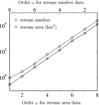
Figure 4: Average area and stream number as functions of stream order for Kentucky River, Kentucky (data taken from Peckham peckham95 ). The stream number data is reversed for simpler comparison with the area data. The Horton ratios are estimated to be $R_{n}\approx R_{a}=4.65\pm 0.05$.

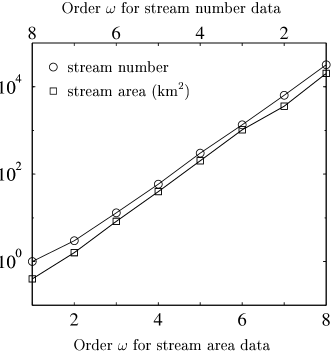
Figure 5: Average area and stream number as functions of stream order for Powder River, Wyoming (data taken from Peckham peckham95 ). Here the ratios are $R_{n}\approx R_{a}=4.55\pm 0.05$.

Note the slight deviation from a linear form for stream numbers for large $\omega$ in both cases. This upwards concavity is as predicted by the modified version of Horton’s law of stream numbers for a single basin, equation (22).

At the other extreme, the fit for both stream areas and stream numbers extends to $\omega=1$. While this may seem remarkable, it is conceivable that at the resolution of the DEM’s used, some orders of smaller streams may have been removed by coarse-graining. Thus, $\omega=1$ may actually be, for example, a third order stream. Note that such a translation in the value of $\omega$ does not affect the determination of the ratios as it merely results in the change of an unimportant multiplicative constant. If $\omega_{r}$ is the true order and $\omega=\omega_{r}-m$, where $m$ is some integer, then, for example,

$$n_{\omega}\propto(R_{n})^{\omega}\sim(R_{n})^{\omega_{r}-m}=\mbox{const}\times(R_{n})^{\omega_{r}}.$$ (31)

This is only a rough argument as coarse-graining does not necessarily remove all streams of low orders.

At odds with the result that $R_{n}\equiv R_{a}$ are past measurements that uniformly find $R_{a}>R_{n}$ at a number of sites. For example, Rosso et al. in rosso91 examine eight river networks and find $R_{a}$ to be on average 40 % greater than $R_{n}$. Clearly, this may be solely due to one or more of the our assumptions not being satisfied. The most likely would be that drainage density is not uniform. However, the limited size of the data sets points to a stronger possibility which we now discuss.

In the case of rosso91 , the networks considered are all third or fourth order basins with one exception of a fifth order basin. As shown by equation (26), if Horton’s laws of stream number and length are exactly followed for all orders, Horton’s law of area is not obeyed for lower orders. Moreover, the former are most likely asymptotic relations themselves. It is thus unsatisfactory to make estimates of Horton’s ratios from only three or four data points taken from the lowest order basins. Note that the Kentucky and Powder rivers are both eighth order networks and thus provide a sufficient range of data.

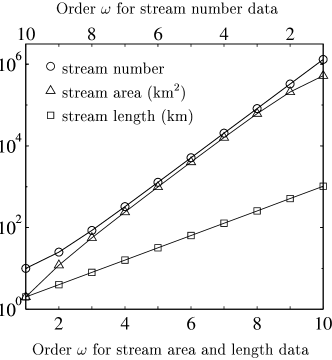
Figure 6: An explanation for the empirical finding that $R_{n}<R_{a}$. Fitting a line to the stream area for only low $\omega$ would result in an overestimate of its asymptotic slope. For stream number, its slope would be underestimated.

We consider more precisely how the corrections to the scaling of area given in equation (27) would affect the measurement of the Horton ratios. Figure 6 shows an example of how stream number, length and area might vary with $\omega$. It is assumed, for the sake of argument, that stream number and length scale exactly as per Horton’s laws and that area behaves as in equation (27), satisfying Horton’s law of area only for higher values of $\omega$. The plot is made for the example values $R_{n}=4$ and $R_{\ell}=2$. The prefactors are chosen arbitrarily so the ordinate is of no real significance.

A measurement of $R_{a}$ from a few data points in the low $\omega$ range will overestimate its asymptotic value as will a similar measurement of $R_{n}$ underestimate its true value. Estimates of $R_{n}$ and $R_{a}$ from a simple least squares fit for various ranges of data are provided in Table 3.

$\omega$ range	$1,2,3$	$1,2,3,4$	$1,2,3,4,5$	$4,5,6,7,8$
$R_{n}$	2.92	3.21	3.41	3.99
$R_{a}$	5.29	4.90	4.67	4.00

Table 3: Values of Horton ratios obtained from least squares estimates of slopes for data represented in Figure 6. The range indicates the data points used in the estimate of the slopes. The ratios obtained from the low order data demonstrate substantial error whereas those obtained from the middle data essentially give the true values of $R_{n}=R_{a}=4$.

Thus, the validity of the methods and results from past work are cast in some doubt. A reexamination of data which has yielded $R_{a}\gg R_{n}$ appears warranted with an added focus on drainage density. Moreover, it is clear that networks of a much higher order must be studied to produce any reasonable results.

VIII Fractal dimensions of networks: a revision

A number of papers and works over the past decade have analyzed the relationships that exist between Horton’s laws and two fractal dimensions used to describe river networks tarboton88 ; labarbera89 ; tarboton90 ; rosso91 ; feder88 ; labarbera94 ; stark97 . These are $D$, the dimension which describes the scaling of the total mass of a network, and ${d}$, the fractal dimension of individual streams that comprises one of our assumptions. In this section, we briefly review these results and point out several inconsistencies. We then provide a revision that fits within the context of our assumptions.

Our starting point is the work of La Barbera and Rosso labarbera89 which was improved by Tarboton et al. to give tarboton90

$$D={d}\frac{\ln R_{n}}{\ln R_{\ell}}.$$ (32)

We find this relation to be correct but that the assumptions and derivations involved need to be redressed. To see this, note that equation (32) was shown to follow from two observations. The first was the estimation of $N(\bar{\ell}_{1})$, the number of boxes of size $\bar{\ell_{1}}\times\bar{\ell_{1}}$ required to cover the network labarbera89 :

$$N(\bar{\ell}_{1})\sim(\bar{\ell}_{1})^{-\ln R_{n}/\ln R_{\ell}}$$ (33)

where $\bar{\ell_{1}}$ is the mean length of first order stream segments. Note that Horton’s laws were directly used in this derivation rather than the correctly modified law of stream numbers for single basins (equation (22)). Nevertheless, the results are the same asymptotically. The next was the inclusion of our second assumption, that single channels are self-affine tarboton90 . Thus, it was claimed, $\bar{\ell}_{1}\sim\delta^{-{d}}$ where $\delta$ is now the length of the measuring stick. Substitution of this into equation (33) gave

$$N(\delta)\sim\delta^{-{d}\ln R_{n}/\ln R_{\ell}},$$ (34)

yielding the stated expression for $D$, equation (32).

However, there is one major assumption in this work that needs to be more carefully examined. The network is assumed to be of infinite order, i.e., one can keep finding smaller and smaller streams. As we have stated, there is a finite limit to the extension of any real network. The possible practical effects of this are pictorially represented in Figure 7. Consider that the network in question is of actual order $\Omega$. Then there are three possible scaling regimes. Firstly, for a ruler of length $\delta\gg\bar{\ell}_{1}$, only the network structure may be detected, given that individual streams are almost one-dimensional. Here, the scaling exponent will be $\ln R_{n}/\ln R_{\ell}$. Next, as $\delta$ decreases, the fractal structure of individual streams may come into play and the exponent would approach that of equation (34). Depending on the given network, this middle section may not even be present or, if so, perhaps only as a small deviation as depicted. Finally, the contribution due to the overall network structure must vanish by the time $\delta$ falls below $\bar{\ell}_{1}$. From this point on, the measurement can only detect the fractal nature of individual streams and so the exponent must fall back to ${d}$.

Figure 7: A schematic representing the problems associated with measuring the fractal dimension of a single river network. Here, the box counting method is assumed and $\delta$, which has the units of length, is the side length of the $N(\delta)$ boxes needed to cover the network. For box sizes much greater than $\bar{\ell}_{1}\times\bar{\ell}_{1}$, only the network structure is detected while for box sizes smaller than $\bar{\ell}_{1}\times\bar{\ell}_{1}$, the measurement picks out the fractal dimension of individual streams. Some deviation towards the scaling suggested by equation (34) may occur between these two limits.

We therefore must rework this derivation of equation (32). As suggested in the definition of ${d}$ in section IV.2, it is more reasonable to treat networks as growing fractals. Indeed, since there is a finite limit to the extent of channelization of a landscape, there is a lower cut-off length scale beyond which most network quantities have no meaning. The only reasonable way to examine scaling behavior is to consider how these quantities change with increasing basin size. This in turn can only be done by comparing different basins of increasing order as opposed to examining one particular basin alone.

With this in mind, the claim that equation (32) is the correct scaling can be argued as follows. Within some basin of order $\Omega$, take a sub-basin of order $\omega$. Consider $N(\omega)$, the number of boxes of side length $\bar{\ell}_{1}$ required to cover the sub-network. This is essentially given by the total length of all the streams in the network. This is given by the approximation of equation (28) and so we have that $N(\omega)\propto(R_{n})^{\omega}$. Using the fact that $\bar{\ell}_{\omega}=(R_{\ell})^{\omega-1}\bar{\ell}_{1}$ we then have that $N(\omega)\propto(\ell_{\omega}/\bar{\ell}_{1})^{\ln R_{n}/\ln R_{\ell}}$. The difference here is that $\bar{\ell}_{1}$ is fixed and pertains to the actual first order streams of the network. By assumption, we have that $\ell_{\omega}\propto L^{{d}}$ and thus

$$N(L)\propto L^{{d}\ln R_{n}/\ln R_{\ell}},$$ (35)

which gives the same value for $D$ as equation (32).

There are two other relations involving fractal dimensions that also need to be reexamined. Firstly Rosso et al. rosso91 found that

$${d}=2\frac{\ln R_{\ell}}{\ln R_{a}}.$$ (36)

Combining equations (32) and (36), they then obtained

$$D=2\frac{\ln R_{n}}{\ln R_{a}}.$$ (37)

However, equation (36) and hence equation (37) are both incorrect.

There is a simple explanation for this discrepancy. In deriving equation (36), Rosso et al. make the assumption that $h={d}/2$, a hypothesis first suggested by Mandelbrot mandelbrot83 . In arriving at the relation $h={d}/2$, Mandelbrot states in mandelbrot83 that “$(\mbox{basin area})^{1/2}$ should be proportional to (distance from source to mouth as the crow flies).” In other words, $a\propto L^{1/2}$. However, as noted in equation (3), observations of real networks show that $a\propto L^{D}$ where $D<2$ maritan96a . Furthermore, on examining the result $h=\ln R_{\ell}/\ln R_{n}$ with the expression for $D$ in equation (32) we see that

$$h=\frac{{d}}{D},$$ (38)

which suggests that this hypothesis is valid only when $D=2$. Consider also the test case of the Scheidegger model where $h=2/3$, $D=3/2$ and ${d}=1$ (see Table 2). Using these values, we see that equation  (38) is exactly satisfied while the relation $h={d}/2$ gives $h=1/2\neq 2/3$.

Now, if $h={d}/D$ is used in place of $h={d}/2$ in deriving equation (36) then equation (32) is recovered. It also follows that equation (37) simplifies to the statement $R_{a}=R_{n}$, further demonstrating the consistency of our derivations. Thus, the two equations (36) and (37) become redundant and the only connection between Horton’s ratios and network dimensions is given by equation (32).

An important point is that $D<2$ does not imply that drainage basins are not space filling. This exponent shows how basin area changes when comparing different basins with different values of $L$, i.e., $a\propto L^{D}$. Any given single basin has of course a fractal dimension of 2. The equating of the way basin sizes change with the actual dimension of any one particular basin is a confusion evident in the literature (see, for example, tarboton88 ). Incorporating the effects of measuring basin area with boxes of side length $\delta$ in the relation $a\propto L^{D}$ would lead to the form

$$a_{L}(\delta)\propto\delta^{-2}L^{D},$$ (39)

where the subscript $L$ has been used to emphasize that different values of $L$ correspond to different basins. Thus, for any given basin (i.e., for fixed $L$), the area scales with $\delta$ while for a fixed $\delta$, areas of different basins scale as per equation (3).

It should also be emphasized that the relationship found here between Hack’s exponent and the fractal dimensions ${d}$ and $D$ is one that is explicitly derived from the assumptions made. The observation that basin areas scale non-trivially with $L$ follows from these starting points and thus there is no need to assume it here.

IX Other scaling laws

We now address three remaining sets of scaling laws. These are probability distributions for areas and stream lengths, scaling of basin shape and Langbein’s law.

As introduced in equation (4), probability distributions for $a$ and $l$ are observed to be power law with exponents $\tau$ and $\gamma$ rodriguez-iturbe97 . Both of these laws have previously been derived from Horton’s laws. De Vries et al. devries94 found a relationship between $\tau$, $R_{n}$ and $R_{\ell}$ but did not include ${d}$ in their calculations while Tarboton et al. tarboton88 obtained a result for $\gamma$ that did incorporate ${d}$.

Again, both of these derivations use Horton’s laws directly rather than the modified version of equation (22). Asymptotically, the same results are obtained from both approaches,

$$\tau=2-\frac{\ln R_{\ell}}{\ln R_{n}}\quad\mbox{and}\quad\gamma=\frac{\ln R_{n}}{\ln R_{\ell}}.$$ (40)

Using the form of the Hack exponent found in equation (38) and equation (32), further connections between these exponents are found:

$$\tau=2-h\quad\mbox{and}\quad\gamma=\frac{1}{h}.$$ (41)

One important outcome concerns the fact that only one of the exponents of the triplet $(h,\tau,\gamma)$ is independent. Previously, for the particular case of directed networks, this has been shown by Meakin et al. meakin91 and further developed by Colaiori et al. colaiori97 . Directed networks are those networks in which all flow has a non-zero positive component in a given direction. In a different setting, Cieplak et al. also arrive at this same conclusion for what they deem to be the separate cases of self-similar and self-affine networks although their assumptions are that $d<1$ and $D<2$ are mutually exclusive contrary to empirical observations cieplak98a . In the case of non-directed networks, Maritan et al. have found one scaling relation for these three exponents, $\gamma=1+(\tau-1)/h$ and, therefore, that two of these three exponents are independent. They further noted that $\tau=2-h$ is an “intriguing result” suggested by real data maritan96a . In the present context, we have obtained this reduction of description in a very general way with, in particular, no assumption regarding the directedness of the networks.

The scaling of basin shapes has been addressed already but it remains to show how it simply follows from our assumptions and how the relevant exponents are related. It is enough to show that this scaling follows from Hack’s law. Now, the area of a basin is related to the longitudinal length $L$ and the width $L_{\perp}$ by $a=L_{\perp}L$, while the main stream length scales by assumption like $l\sim L^{{d}}$. Hence,

$$l\sim a^{h} \Rightarrow L^{{d}}\sim(L_{\perp}L)^{h}$$ (42)

$$\Rightarrow L_{\perp}\sim L^{{d}/h-1}=L^{D-1}$$

where the fact that $h={d}/D$ has been used. Comparing this to equation (3) we obtain the scaling relation

$$H=D-1.$$ (43)

The last set of exponents we discuss are those relating to Langbein’s law langbein47 . Langbein found that $\tilde{\Lambda}$, the sum of the distances (along streams) from stream junctions to the outlet of a basin, scales with the area of the basin. Recently, Maritan et al. maritan96a introduced the quantity $\lambda$, which is an average of Langbein’s $\tilde{\Lambda}$ except now the sum is taken over all points of the network. Citing the case of self-organized critical networks, they made the claim that

$$\lambda\propto L^{\varphi}.$$ (44)

Further, they assumed that $\varphi={d}$ although it was noted that there is no clear reason why this may be so since there are evident differences in definition ($\lambda$ involves distances downstream while ${d}$ involves distances upstream). We find this scaling relation to hold in the present framework. We further consider the two related quantities $\Lambda$ and $\tilde{\lambda}$, respectively the sum over all points and the average over all junctions of distances along streams to the basin outlet.

The calculations are straightforward and follow the manner of previous sections. We first calculate $\lambda(\omega,\Omega)$, the typical distance to the outlet from a stream of order $\omega$ in an order $\Omega$ basin. Langbein’s $\tilde{\Lambda}$, for example, is then obtained as $\sum_{\omega=1}^{\Omega}n(\omega,\Omega)\lambda(\omega,\Omega)$. We find the same scaling behavior regardless of whether sums are taken over all points or all junctions. Specifically we find

$$\Lambda\sim\tilde{\Lambda}\sim a^{1+\ln R_{\ell}/\ln R_{n}}\quad\mbox{and}\quad\lambda\sim\tilde{\lambda}\sim L^{d}$$ (45)

yielding the scaling relations

$$\beta=\tilde{\beta}={1+\ln R_{\ell}/\ln R_{n}}\quad\mbox{and}\quad\tilde{\varphi}=\varphi={d}.$$ (46)

Note that the second pair of scaling relations admit other methods of measuring ${d}$. The large amount of averaging inherent in the definition of the quantity $\lambda$ would suggest that it is a more robust method for measuring ${d}$ than one based on measurements of the sole main stream of the basins.

Maritan et al. maritan96a provide a list of real world measurements for various exponents upon which several comments should be made. Of particular note is the relationship between $\tau=2-h$. This is well met by the cited values $1.41<\tau<1.45$ and $0.57<h<0.60$. Also reasonable is the estimate of $h$ given by ${d}/D$ ($D=\phi$ in their notation) which is $0.58<h<0.65$.

The values of $\gamma$ and $\varphi$, however, do not work quite so well. The latter does not match ${d}$ within error bars, although they are close in absolute value with $\varphi=1.05\pm 0.01$ and ${d}=1.10\pm 0.01$. The length distribution exponent $\gamma$ may be found via 3 separate routes: $\gamma=1/h=D/{d}=1/(2-\tau)$. The second and third equalities have been noted to be well satisfied and so any one of the 3 estimates of $\gamma$ may be used. Take, for example, the range $0.58<h<0.59$, which falls within that given by $h=2-\tau$, $h={d}/D$ and the range given for $h$ itself. This points to the possibility that the measured range $1.8<\gamma<1.9$ is too high, since using $\gamma=1/h$ yields $\gamma=1.74\pm.02$. Also of note is that Maritan et al.’s own scaling relation $\gamma=1+(\tau-1)/h$ would suggest $\gamma=1.74\pm.05$.

Better general agreement with the scaling relations is to be found in rigon96 in which Rigon et al. detail specific values of $h$, $\tau$ and $\gamma$ for some thirteen river networks. Here, the relations $\tau=2-h$ and $\gamma=1/h$ are both well satisfied. Comparisons for this set of data show that, on average and given the cited values of $h$, both $\tau$ and $\gamma$ are overestimated by only 2 per cent.

X Concluding remarks

We have demonstrated that the various laws, exponents and parameters found in the description of river networks follow from a few simple assumptions. Further, all quantities are expressible in terms of two fundamental numbers. These are a ratio of logarithms of Horton’s ratios, $\ln R_{n}/\ln R_{\ell}$, and the fractal dimension of individual streams, ${d}$. There are only two independent parameters in network scaling laws. These Horton ratios were shown to be equivalent to Tokunaga’s law in informational content with the attendant assumption of uniform drainage density. Further support for this observation is that both the Horton and Tokunaga descriptions depend on two parameters each and an invertible transformation between them exists (see equations (12), (15) and (17)). A summary of the connections found between the various exponents is presented in Table 4.

It should be emphasized that the importance of laws like that of Tokunaga and Horton in the description of networks is that they provide explicit structural information. Other measurements such as the power law probability distributions for length and area provide little information about how a network fits together. Indeed, information is lost in the derivations as the Horton ratios cannot be recovered from knowledge of $\ln R_{n}/\ln R_{\ell}$ and ${d}$ only.

The basic assumptions of this work need to be critically examined. Determining how often they hold and why they hold will follow through to a greater understanding of all river network laws. One vital part of any river network theory that is lacking here is the inclusion of the effects of relief, the third dimension. Another is the dynamics of network growth: why do mature river networks exhibit a self-similarity that gives rise to these scaling laws with these particular values of exponents? Also, extensive studies of variations in drainage density are required. The assumption of its uniformity plays a critical role in the derivations and needs to be reexamined. Lastly, in those cases where these assumptions are valid, the scaling relations gathered here provide a powerful method of cross-checking measurements.

Finally, we note that work of a similar nature has recently been applied to biological networks west97 . The assumption analogous to network self-similarity used in the biological setting is considerably weaker as it requires only that the network is a hierarchy. A principle of minimal work is then claimed to constrain this hierarchy to be self-similar. It is conceivable that a similar approach may be found in river networks. However, a generalization of the concept of a hierarchy and perhaps stream ordering needs to be developed since a ‘Tokunagic network’ is not itself a simple hierarchy.

law:	parameter in terms of $R_{n}$, $R_{\ell}$ and ${d}$:
$T_{\nu}=T_{1}(R_{T})^{\nu-1}$	$T_{1}=R_{n}-R_{\ell}-2+2R_{\ell}/R_{n}$
	$R_{T}=R_{\ell}$
$l\sim L^{{d}}$	—
$n_{\omega+1}/n_{\omega}=R_{n}$	—
$\bar{\ell}_{\omega+1}/\bar{\ell}_{\omega}=R_{\ell}$	—
$\bar{l}_{\omega+1}/\bar{l}_{\omega}=R_{\ell}$	—
$\bar{a}_{\omega+1}/\bar{a}_{\omega}\sim R_{a}$	$R_{a}=R_{n}$
$l\sim a^{h}$	$h=\ln R_{\ell}/\ln R_{n}$
$a\sim L^{D}$	$D={d}\ln R_{n}/\ln R_{\ell}$
$L_{\perp}\sim L^{H}$	$H={d}\ln R_{n}/\ln R_{\ell}-1$
$P(a)\sim a^{-\tau}$	$\tau=2-\ln R_{\ell}/\ln R_{n}$
$P(l)\sim l^{-\gamma}$	$\gamma=\ln R_{n}/\ln R_{\ell}$
$\Lambda\sim a^{\beta}$	$\beta=1+\ln R_{\ell}/\ln R_{n}$
$\lambda\sim L^{\varphi}$	$\varphi={d}$
$\tilde{\Lambda}\sim a^{\tilde{\beta}}$	$\tilde{\beta}=1+\ln R_{\ell}/\ln R_{n}$
$\tilde{\lambda}\sim L^{\tilde{\varphi}}$	$\tilde{\varphi}={d}$

Table 4: Summary of scaling laws and the scaling relations found between the various exponents. Compare with table 1.

References

- (1) B. B. Mandelbrot, The Fractal Geometry of Nature (Freeman, San Francisco, 1983).
- (2) R. E. Horton, Bull. Geol. Soc. Am 56(3), 275 (1945).
- (3) W. B. Langbein, U.S. Geol. Surv. Water-Supply Pap. W 0968-C, 125 (1947).
- (4) A. N. Strahler, Bull. Geol. Soc. Am 63, 1117 (1952).
- (5) J. T. Hack, U.S. Geol. Surv. Prof. Pap. 294-B, 45 (1957).
- (6) D. G. Tarboton, R. L. Bras, and I. Rodríguez-Iturbe, Water Resour. Res. 24(8), 1317 (1988).
- (7) P. La Barbera and R. Rosso, Water Resour. Res. 25(4), 735 (1989).
- (8) D. G. Tarboton, R. L. Bras, and I. Rodríguez-Iturbe, Water Resour. Res. 26(9), 2243 (1990).
- (9) A. Maritan, A. Rinaldo, R. Rigon, A. Giacometti, and I. Rodríguez-Iturbe, Phys. Rev. E 53(2), 1510 (1996).
- (10) L. B. Leopold and W. B. Langbein, U.S. Geol. Surv. Prof. Pap. 500-A, 1 (1962).
- (11) R. L. Shreve, J. Geol. 74, 17 (1966).
- (12) A. D. Howard, Geogr. Anal. 3, 29 (1971).
- (13) C. P. Stark, Nature 352, 405 (1991).
- (14) P. Meakin, J. Feder, and T. Jøssang, Physica A 176, 409 (1991).
- (15) G. Willgoose, R. L. Bras, and I. Rodríguez-Iturbe, Water Resour. Res. 27(7), 1685 (1991).
- (16) G. Willgoose, R. L. Bras, and I. Rodríguez-Iturbe, Earth Surf. Proc. Landforms 16, 237 (1991).
- (17) G. Willgoose, R. L. Bras, and I. Rodríguez-Iturbe, Water Resour. Res. 27(7), 1671 (1991).
- (18) S. Kramer and M. Marder, Phys. Rev. Lett. 68(2), 205 (1992).
- (19) R. L. Leheny and S. R. Nagel, Phys. Rev. Lett. 71(9), 1470 (1993).
- (20) T. Sun, P. Meakin, and T. Jøssang, Phys. Rev. E 49(6), 4865 (1994).
- (21) T. Sun, P. Meakin, and T. Jøssang, Water Resour. Res. 30(9), 2599 (1994).
- (22) E. Somfai and L. M. Sander, Phys. Rev. E 56(1), R5 (1997).
- (23) I. Rodríguez-Iturbe and A. Rinaldo, Fractal River Basins: Chance and Self-Organization (Cambridge University Press, Great Britain, 1997).
- (24) P. Bak, How Nature Works: the Science of Self-Organized Criticality (Springer-Verlag, New York, 1996).
- (25) A. E. Scheidegger, International Association of Scientific Hydrology Bulletin 12(1), 15 (1967).
- (26) A. E. Scheidegger, Theoretical Geomorphology (Springer-Verlag, New York, 1991), third ed.
- (27) A. N. Strahler, EOS Trans. AGU 38(6), 913 (1957).
- (28) M. A. Melton, J. Geol. 67, 345 (1959).
- (29) D. M. Gray, J. Geophys. Res. 66(4), 1215 (1961).
- (30) R. Rigon, I. Rodríguez-Iturbe, A. Maritan, A. Giacometti, D. G. Tarboton, and A. Rinaldo, Water Resour. Res. 32(11), 3367 (1996).
- (31) J. E. Mueller, Geological Society of America Bulletin 83, 3471 (1972).
- (32) M. P. Mosley and R. S. Parker, Geological Society of America Bulletin 84, 3123 (1973).
- (33) J. E. Mueller, Geological Society of America Bulletin 84, 3127 (1973).
- (34) P. La Barbera and R. Rosso, Water Resour. Res. 26(9), 2245 (1990).
- (35) E. Tokunaga, Geophys. Bull. Hokkaido Univ. 15, 1 (1966).
- (36) E. Tokunaga, Geogr. Rep., Tokyo Metrop. Univ. 13, 1 (1978).
- (37) E. Tokunaga, Trans. Jpn. Geomorphol. Union 5(2), 71 (1984).
- (38) S. D. Peckham, Water Resour. Res. 31(4), 1023 (1995).
- (39) W. I. Newman, D. L. Turcotte, and A. M. Gabrielov, Fractals 5(4), 603 (1997).
- (40) A. E. Scheidegger, Water Resour. Res. 4(5), 1015 (1968).
- (41) J. W. Kirchner, Geology 21, 591 (1993).
- (42) S. A. Schumm, Bull. Geol. Soc. Am 67, 597 (1956).
- (43) H. Takayasu, I. Nishikawa, and H. Tasaki, Phys. Rev. A 37(8), 3110 (1988).
- (44) M. Takayasu and H. Takayasu, Phys. Rev. A 39(8), 4345 (1989).
- (45) H. Takayasu, Physcial Review Letters 63(23), 2563 (1989).
- (46) H. Takayasu, Fractals in the Physical Sciences (Manchester University Press, Manchester, 1990).
- (47) H. Takayasu, M. Takayasu, A. Provata, and G. Huber, J. Stat. Phys. 65(3/4), 725 (1991).
- (48) G. Huber, Physica A 170, 463 (1991).
- (49) A. D. Abrahams, Water Resour. Res. 20(2), 161 (1984).
- (50) D. R. Montgomery and W. E. Dietrich, Science 255, 826 (1992).
- (51) D. G. Tarboton, R. L. Bras, and I. Rodríguez-Iturbe, Water Resour. Res. 25(9), 2037 (1989).
- (52) R. L. Shreve, J. Geol. 75, 178 (1967).
- (53) P. Haggett and R. J. Chorley, Network Analysis in Geography (Edward Arnold, London, 1969).
- (54) V. Gardiner, Geogr. Ann. 55A(3–4), 147 (1973).
- (55) M. E. Morisawa, Geological Society of America Bulletin 73, 1025 (1962).
- (56) H. de Vries, T. Becker, and B. Eckhardt, Water Resour. Res. 30(12), 3541 (1994).
- (57) W. S. Glock, The Geogr. Rev. 21, 475 (1931).
- (58) P. S. Dodds, R. Pastor-Satorras, and D. H. Rothman, Fluctuation in River network scaling laws (1999), in preparation.
- (59) R. Rosso, B. Bacchi, and P. La Barbera, Water Resour. Res. 27(3), 381 (1991).
- (60) J. S. Smart, Water Resour. Res. 3(3), 773 (1967).
- (61) J. Feder, Fractals (Plenum Press, New York, 1988).
- (62) P. La Barbera and G. Roth, Hydrol. Processes 8, 125 (1994).
- (63) C. P. Stark, Stream networks on a Bethe lattice: Cayley trees, invasion percolation and branching ratios (1997), preprint.
- (64) F. Colaiori, A. Flammini, A. Maritan, and J. R. Banavar, Phys. Rev. E 55(2), 1298 (1997).
- (65) M. Cieplak, A. Giacometti, A. Maritan, A. Rinaldo, I. Rodríguez-Iturbe, and J. R. Banavar, J. Stat. Phys. 91(1/2), 1 (1998).
- (66) G. B. West, J. H. Brown, and B. J. Enquist, Science 276, 122 (1997).