Enhancement of quantum dot peak-spacing fluctuations in the fractional quantum Hall regime

Abstract

The fluctuations in the spacing of the tunneling resonances through a quantum dot have been studied in the quantum Hall regime. Using the fact that the ground-state of the system is described very well by the Laughlin wavefunction, we were able to determine accurately, via classical Monte Carlo calculations, the amplitude and distribution of the peak-spacing fluctuations. Our results clearly demonstrate a big enhancement of the fluctuations as the importance of the electronic correlations increases, namely as the density decreases and filling factor becomes smaller. We also find that the distribution of the fluctuations approaches a Gaussian with increasing density of random potentials.

Several experimental studies[1, 2, 3] have recently demonstrated that the fluctuations in the ground-state energy of a quantum dot, which are manifested in the fluctuations in the resonant-tunneling-peak spacings, are much larger than what one expect from models that ignore electron correlations. Numerical studies[1, 4, 5, 6] have indeed revealed an enhancement of the ground-state energy fluctuations due to electron-electron interactions.

In this work we present calculations for an interacting electron system in a regime that can be treated almost exactly - the quantum Hall regime. The ground-state wavefunction in this regime is faithfully described by the Laughlin wavefunction [7]. Consequently, as long as the potential fluctuations do not mix in excited states (i.e. when the potential energy is smaller than the gap), the peak-spacing fluctuations (PSF) can be evaluated as expectation values in the Laughlin state. As such expectation values can be easily calculated using the plasma analogy [7], via, e.g., classical Monte Carlo simulations, we are able to obtain the magnitude of the PSF, their distribution and their dependence on the range of the potentials and the electron number. Indeed we find that the more important the electronic correlations (the lower the filling factor), the larger the magnitude of the PSF. In addition, we also find that the distribution of PSF is Gaussian, in agreement with experiments [1, 2, 3].

The experimentally measured quantity is the spacings between the resonant-tunneling peaks through the quantum dot. At low enough temperatures (smaller than the excitation energies of the dot), the peak spacing is determined by the addition spectrum,

$$\Delta_{2}^{\scriptscriptstyle(N)}\equiv\left(E_{g}^{\scriptscriptstyle(N+1)}-E_{g}^{\scriptscriptstyle(N)}\right)-\left(E_{g}^{\scriptscriptstyle(N)}-E_{g}^{\scriptscriptstyle(N-1)}\right),$$ (1)

where $E_{g}^{\scriptscriptstyle(N)}$ is the ground-state energy of the N-particle system. In the constant-interaction model [8] $E_{g}^{\scriptscriptstyle(N)}=N(N-1)U/2+\sum_{i}^{N}\epsilon_{i}$, where $U$ is the charging energy and $\epsilon_{i}$ is the single-electron spectrum. In this model the peak-spacing fluctuations are determined by the fluctuations in the single-electron spectrum, which are described by random-matrix theory, in contrast with the experimental observations. This deviation from random-matrix theory was attributed to the importance of electronic correlations, which are not captured in the constant-interaction model.

For strong magnetic fields, in particular in the fractional quantum Hall regime, electronic correlations become very significant and dominate the underlying physics. The ground-state wavefunction of $N$ electrons in a quantum dot in a strong magnetic field, with filling factor $\nu=1/m$, can be described very well by the Laughlin wavefunction [7]

$$\Psi^{(\scriptscriptstyle 1/m)}\left(z_{1},...,z_{N}\right)=\prod_{i<j}\,(z_{i}-z_{j})^{m}\ e^{-\sum_{i}|z_{i}|^{2}/4},$$ (2)

where $z_{i}$ denotes the complex coordinates of the $i$-th particle, $z_{i}=x_{i}+iy_{i}$, and all lengths are expressed in units of the magnetic length, $\ell_{H}\equiv\sqrt{\hbar c/eH}$.

Since the magnetic field quenches the kinetic energy and the interaction energy varies smoothly with the number of particles, the fluctuations in the peak spacings stem only from fluctuations in the potential energy. If the energy gap due to correlations is large enough (compared to the potential), the potential energy in the presence of a random potential $V(z)$, is given by $E_{pot}^{\scriptscriptstyle(N)}=\int d^{2}r\rho_{\scriptscriptstyle N}^{\scriptscriptstyle(1/m)}(r)V(\stackrel{{\scriptstyle\rightarrow}}{{r}})$, where $\rho_{\scriptscriptstyle N}^{\scriptscriptstyle(1/m)}(r)$ is the single-particle distribution function,

$$\rho_{\scriptscriptstyle N}^{\scriptscriptstyle(1/m)}(r)=\int d^{2}z_{1}\ldots d^{2}z_{N}\ |\Psi^{(\scriptscriptstyle 1/m)}\left(z_{1},...,z_{N}\right)|^{2}\ \delta(|z_{1}|^{2}-r^{2})$$ (3)

The single-particle distribution $\rho_{\scriptscriptstyle N}^{\scriptscriptstyle(1/m)}(r)$ can be calculated using the mapping onto a classical plasma model [7]. This mapping is based upon rewriting $|\Psi|^{2}$ as

$$|\Psi^{(\scriptscriptstyle 1/m)}\left(z_{1},...,z_{N}\right)|^{2}=\exp\left[-\sum_{i}|z_{i}|^{2}/2+m\sum_{i<j}\log(|z_{i}-z_{j}|^{2})\right].$$ (4)

Consequently, expectation values in the ground-state can be expressed as statistical averages for a classical system of $N$ particles in a harmonic confining potential and logarithmic interactions. These averages were evaluated using a classical Monte Carlo approach [9].

Fig. 1.–: (a) Single-particle densities for 15, 20 and 25 particles in the $\nu=1/3$ quantum Hall regime. (b) The same densities as in (a), but relatively shifted (see text).

In fig. 1a we plot the single-particle density of 15, 20 and 25 particles in the $\nu=1/3$ fractional quantum Hall regime. As can be seen from the figure, the bulk density is constant, while the edge structure for different particle numbers is identical, but relatively shifted. Since the edge of the $N$-particle system in the $\nu=1/m$ case is determined by the maximal occupied angular momentum state, $m(N-1)$, localized at distance $\sqrt{2m(N-1)}$ from the origin, the edge structure of $N_{1}$ and $N_{2}$-particle systems can be made to collapse by a relative shift of $\sqrt{2m(N_{1}-1)}-\sqrt{2m(N_{2}-1)}$. In fig. 1b we replot the same densities as in fig. 1a, but relatively shifted in that manner. Indeed we see that all the distributions collapse onto a single curve. This invariance of the edge-structure allows us to deduce immediately the $N$-dependence of the peak-spacing fluctuations: writing

$$\Delta_{2}^{\scriptscriptstyle(N)}=\int d^{2}r\ \Delta_{2}\rho_{\scriptscriptstyle N}^{\scriptscriptstyle(1/m)}(r)\ V(\stackrel{{\scriptstyle\rightarrow}}{{r}})\simeq\int d^{2}r\ {{\partial^{2}\rho_{\scriptscriptstyle N}^{\scriptscriptstyle(1/m)}(r)}\over{\partial N^{2}}}\ V(\stackrel{{\scriptstyle\rightarrow}}{{r}}),$$ (5)

(with $\Delta_{2}\rho_{\scriptscriptstyle N}\equiv\rho_{\scriptscriptstyle N+1}+\rho_{\scriptscriptstyle N-1}-2\rho_{\scriptscriptstyle N}$), and using the abovementioned fact that

$$\rho_{\scriptscriptstyle N}^{\scriptscriptstyle(1/m)}(r)=\rho_{\scriptscriptstyle N_{0}}^{\scriptscriptstyle(1/m)}(r+\sqrt{2m(N_{0}-1)}-\sqrt{2m(N-1)}),$$ (6)

one finds, after a little algebra, that for short-range potentials and large $N$ the fluctuations in $\Delta_{2}$ scale like $<(\Delta_{2}^{\scriptscriptstyle(N)})^{2}>\sim N^{\scriptscriptstyle-3/2}$. Here $<...>$ denotes average over realizations of the random potential. In particular, for delta-function potentials of density $n_{0}$ and typical strength $V_{0}$, one finds $<(\Delta_{2}^{\scriptscriptstyle(N)})^{2}>=A_{m}n_{0}V_{0}^{2}N^{-3/2}$, where $A_{m}$ is $N$-independent for large $N$.

Fig. 2.–: (a) Averaged peak-spacing fluctuations for $\nu=1,1/3$, and $1/5$. The continuous lines are fits to $A_{m}/N^{3/2}$ ($\nu=1/3$ and $1/5$) and the exact result for $\nu=1$. (b) The same data as in (a), normalized by the large-$N$ $\nu=1$ exact result.

In fig. 2a we show the averaged PSF, $<(\Delta_{2}^{\scriptscriptstyle(N)})^{2}>$, in the $\nu=1,\ 1/3$ and $1/5$ quantum Hall regimes. In agreement with the above argument, the average PSF scale with $N^{-3/2}$ (continuous curve). In fig. 2b we plot the numerically calculated $A_{m}$ (scaled by the large-$N$ value $A_{1}\rightarrow 1/8\pi^{\scriptscriptstyle 3/2}$) as a function of $N$. As expected, it is indeed $N$-independent within the accuracy of the calculation. The numerically deduced values lead to

$$<(\Delta_{2}^{\scriptscriptstyle(N)})^{2}>_{1/3}/<(\Delta_{2}^{\scriptscriptstyle(N)})^{2}>_{1} = 5.0\pm 0.3$$

$$<(\Delta_{2}^{\scriptscriptstyle(N)})^{2}>_{1/5}/<(\Delta_{2}^{\scriptscriptstyle(N)})^{2}>_{1} = 9.2\pm 0.5.$$ (7)

These calculations clearly demonstrate the enhancement of the PSF due to the increased role of correlations, as the filling factor is lowered [10]. (Note that the PSF are independent of the charging energy in this regime).

As the range of the random potentials, $\sigma$, increases, the PSF are reduced and the ratios (eq.(7)) decrease towards unity (fig. 3). However, once $\sigma$ becomes of the order of the size of the dot, $R\propto\sqrt{N}$, the PSF become independent of system size and the ratio increase again, leading to a nonmonotonic dependence on $\sigma$. In the limit of very smooth potentials, $\sigma\rightarrow\infty$, one can show that the PSF are given by

$$<(\Delta_{2}^{\scriptscriptstyle(N)})^{2}>={5\pi<V_{0}^{2}>n_{0}\over{16\sigma^{6}}}\left(\int d^{2}r\ r^{2}\ \Delta_{2}\rho_{\scriptscriptstyle N}^{\scriptscriptstyle(1/m)}(r)\right)^{2}\ .$$ (8)

The quantity in parentheses is twice the second derivative of the total angular momentum with respect to $N$ and is equal to $2m$. Thus in this limit, one finds

$$<(\Delta_{2}^{\scriptscriptstyle(N)})^{2}>_{1/3}/<(\Delta_{2}^{\scriptscriptstyle(N)})^{2}>_{1} = 9$$

$$<(\Delta_{2}^{\scriptscriptstyle(N)})^{2}>_{1/5}/<(\Delta_{2}^{\scriptscriptstyle(N)})^{2}>_{1} = 25,$$ (9)

namely there is an enhancement of the PSF also in this limit. As the range of the potentials is determined experimentally by the distance to the donor layer, which is of the same order of the dot size, the ratio $\sigma/R$ can be varied experimentally in the relevant regime and these predictions, including the nonmonotonicity, could be tested.

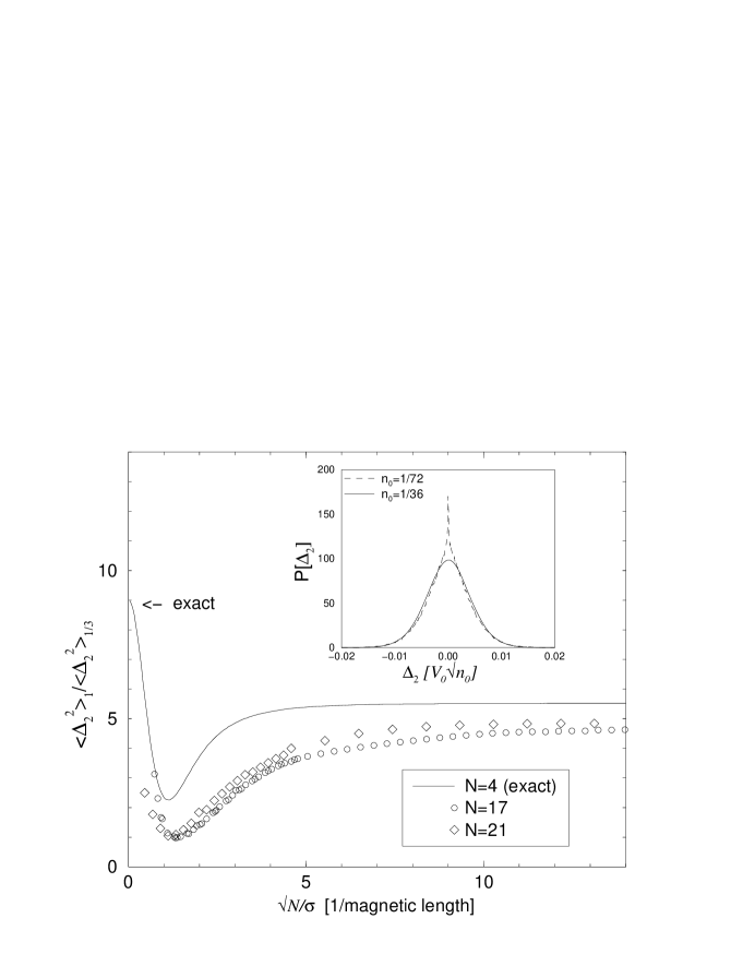
Fig. 3.–: The ratio of the average peak-spacing fluctuations between the $\nu=1$ and the $\nu=1/3$ quantum Hall regimes as a function of the range of the potentials, scaled by the dot size $R\propto\sqrt{N}$. inset: The distribution of the peak-spacing fluctuations for two densities of random potentials. For the larger densities the distribution approaches a Gaussian.

The observed features can be understood as follows. Based on Wen’s description of the edges of the quantum Hall liquid [11], Kinaret et al. have shown that for filling factors $\nu=1/m$, $\Delta_{2}=mv/R$, where $R$ is the radius of the system and $v$ the edge velocity. This result can be simply understood – when the number of particles increases by one, the energy of the highest-occupied angular momentum state increases by $\nabla V\partial R/\partial N$, where $\nabla V$ is the potential gradient near the edge of the system. Since $R\sim\sqrt{2mN}$ this immediately leads to $\Delta_{2}\sim m\nabla V/R\propto mv/R$. This result implies $<(\Delta_{2})^{2}>\sim m^{2}<(\nabla V)^{2}>/N$. As $<(\nabla V)^{2}>\sim n<V_{0}^{2}>/\sigma^{6}$, where $n$ is the number of random potentials, one immediately reproduces eq.(8). As the derivation here relied on the sharpness of the edge it only strictly applies in that limit. For finite-range potentials one expects the internal structure of the edge to modify this result, which in indeed observed numerically.

Lastly we consider the full distribution of the PSF. For simplicity, we concentrate on delta-function potentials. In this case the distribution is defined by

$$P(\Delta_{2})\equiv\int\ \prod_{i}d^{2}r_{i}\ dV_{i}\ P(r_{i},V_{i})\ \ \delta\left(\Delta_{2}-\sum_{i}V_{i}\Delta_{2}\rho(r_{i})\right),$$ (10)

where $P(r_{i},V_{i})$ is the probability of finding a delta-potential of magnitude $V_{i}$ at point $r_{i}$. Assuming a uniform distribution of potentials of density $n_{0}$, and a Gaussian distribution of their amplitudes, with width $V_{0}$, one finds

$$P(\Delta_{2})=\int\ \prod_{i}{d^{2}r_{i}\over A}\ {1\over\sqrt{2\pi\Sigma}}\ e^{-\Delta_{2}^{2}/(2\Sigma^{2})};\ \ \ \Sigma\equiv V_{0}^{2}\ \sum_{i}\left(\Delta_{2}\rho(r_{i})\right)^{2}.$$ (11)

When the potentials are dense, the sum (in the expression for $\Sigma$) can be approximated by an integral, and we immediately find that the $\Delta_{2}$ is distributed normally with a width that has been calculated above. Note that this derivation did not involve any information about the quantum Hall system (except the assumption that one can treat the potential fluctuations perturbatively), and is just a manifestation of the law of big numbers.

When the density of the potentials is lowered, there is a finite probability that none of the potentials affects the region of interest – the edge of the system. This enhances the probability that $\Delta_{2}=0$. In the inset of fig. 3 we plot the distribution of the PSF for two different densities of potentials. We indeed see that for low enough density there is a sharp peak at $\Delta_{2}=0$, while the distribution approaches a Gaussian for large enough density. We expect a similar effect when the range of the potential increases.

To conclude, we have demonstrated that the increased importance of the correlations in the quantum Hall regime leads to an enhancement of the peak-spacing fluctuations. This can be attributed to the increased rigidity of the ground-state wavefunction as the filling factor becomes lower.

1 acknowledgements

This research was supported by THE ISRAEL SCIENCE FOUNDATION founded by the Israel Academy of Sciences and Humanities - Centers of Excellence Program.

References

- [1] Sivan U., et al.: , Phys. Rev. Lett., 77 (1996) 1123.
- [2] Simmel F., Heinzel T. and Wharam D. A., Europhys. Lett., 38 (1997) 123.
- [3] Patel S. R., et al.: , condmat/9708090,.
- [4] Prus O., et al.: , Phys. Rev., B 54 (1996) R14289; Berkovits R. and Sivan U., Europhys. Lett., 41 (1998) 653; Berkovits R., condmat/9804107,.
- [5] Koulakov A. A., Pikus F. G. and Shklovskii B. I., Phys. Rev., B 55 (1997) 9223.
- [6] See, however, Blanter Ya. M., Mirlin A. D. and Muzykantskii B. A., Phys. Rev. Lett., 78 (1997) 2449; Vallejos R. O., Lewenkopf C. H. and Mucciolo E. R., condmat/9802124,.
- [7] R.B. Laughlin, Phys. Rev. Lett., 50 (1983) 1395.
- [8] For a review see: M. A. Kastner, Rev. Mod. Phys., 64 (1992) 849.
- [9] M. Metropolis et al.: , J. Chem. Phys., 21 (1953) 1087.
- [10] Throughout this paper we assume that the change in filling factor is caused by a change in density (gate-voltage), with constant magnetic field. If the magnetic field is also changed, trivial factors that involve the respective magnetic lengths will enter the ratios in eqs. (7) and (9). In fact, if the change in filling factor is fully caused by a change in the magnetic field, there will be no dependence of the PSF on the filling factor in the limit of very smooth potentials.
- [11] For a review see X.-G. Wen, Int. J. Mod. Phys., 6 (1992) 1711.
- [12] Kinaret J. M., et al.: , Phys. Rev., B 46 (1992) 4681.