Thermodynamics of glasses: a first principle computation

Abstract

We propose a first principle computation of the thermodynamics of simple fragile glasses starting from the two body interatomic potential. A replica formulation translates this problem into that of a gas of interacting molecules, each molecule being built of $m$ atoms, and having a gyration radius (related to the cage size) which vanishes at zero temperature. We use a small cage expansion, valid at low temperatures, which allows to compute the cage size, the specific heat (which follows the Dulong and Petit law), and the configurational entropy.

Take a three dimensional classical system consisting of $N$ particles, interacting by pairs through a short range potential. Very often this system will undergo, upon cooling or upon density increasing, a solidification into an amorphous solid state- the glass state. The conditions required for observing this glass phase is the avoidance of crystallisation, which can always be obtained through a fast enough quench (the meaning of ’fast’ depends very much of the type of system) [3]. There also exist potentials which naturally present some kind of frustration with respect to the crystalline structures and therefore solidify into glass states, even when cooled slowly- such is the case for instance of binary mixtures of hard spheres, soft spheres, or Lennard-Jones particles with appropriately different radii. These have been studied a lot in recent numerical simulations [4, 5, 6, 7, 8].

Our aim is to compute the thermodynamic properties of this glass phase, using the statistical mechanical approach, namely starting from the microscopic Hamiltonian. The general framework of our approach finds its roots in old ideas of Kauzman [10], Adam and Gibbs [11], which received a boost when Kirkpatrick, Thirumalai and Wolynes underlined the analogy between structural glasses and some generalized spin glasses [12]. In this framework, which should provide a good description of fragile glass-formers, the glass transition, measured from dynamical effects, is associated with an underlying thermodynamic transition at the Kauzman or Vogel-Fulcher temperature $T_{K}$. This ideal glass transition is the one which should be observed on infinitely long time scales [3]. This transition is of an unusual type, since it presents two apparently contradictory features: 1) The order parameter is discontinuous at the transition: defining the order parameter as the inverse radius of the cage seen by each particle, it jumps discontinuously from $0$ in the liquid phase to a finite value in the glass phase. 2) The transition is continuous (second order) from the thermodynamical point of view: the free energy is continuous, and the transition is signalled by a discontinuity of the specific heat which jumps from its liquid value above $T_{s}$ to a value very close to that of a crystal phase below. These properties are indeed observed in generalized spin glasses [13]. The problem of the existence or not of a diverging correlation length is still an open one [14].

This analogy is suggestive, but it also hides some very basic differences, like the fact that spin glasses have quenched disorder while structural glasses do not. The recent discovery of some generalized spin glass systems without quenched disorder [15] has given credit to the idea that this analogy is not fortuitous. The problem was to turn this general idea into a consistent computational scheme allowing for some quantitative predictions. Important steps in this direction were invented in [19, 18], which showed the necessity of using several copies of the same system in order to define properly the glass phase. In a previous preliminary study, we used some of these ideas to estimate the glass temperature, arriving from the liquid phase [25]. Here we concentrate instead on the properties of the glass phase itself, and particularly its properties at low temperatures.

The Hamiltonian of our problem is simply given by:

$$H=\sum_{1\leq i\leq j\leq N}v(x_{i}-x_{j})$$ (1)

where the particles move in a volume $V$ of a d-dimensional space, and $v$ is an arbitrary short range potential. We shall take the thermodynamic limit $N,V\to\infty$ at fixed density $\rho=N/V$. For simplicity, we do not consider here the description of mixtures, which is presumably an easy generalisation. The main obstacle to a study of the glass phase is the very description of the amorphous solid state. In principle one should give the average position of each atom in the solid, which requires an infinite amount of information. Had we known this information, we could have added to the Hamiltonian an infinitesimal but extensive pinning field which attracts each particle to its equilibrium position, sending $N$ to infinity first, before taking the limit of zero pinning field. This is the usual way of identifying the phase transition. In order to get around the problem of the description of the amorphous solid phase, a simple method has been developed in the spin glass context- although one does not know the conjugate field, the system itself will know it, and the idea is to consider two copies (sometimes called ’replicas’) of the system, with an infinitesimal extensive attraction. In the spin glass case this is a very nice method which allows to identify the transition temperature from the fact that the two replicas remain close to each other in the limit of vanishing coupling [26, 27].

However this method is too naive and needs to be modified for the case of glasses. The reason has to do with the degeneracy of glass states. This property can be studied in detail in generalized spin glass mean field models [17, 16]. For structural glasses, this is a conjecture which we shall make, on the basis of its agreement with the phenomenology of glasses [8]. Let us assume that we can introduce a free energy functional $F(\rho)$ which depends on the density $\rho(x)$ and on the temperature. We suppose that at sufficiently low temperature this functional has many minima (i.e. the number of minima goes to infinity with the number $N$ of particles). Exactly at zero temperature these minima coincide with the mimima of the potential energy as function of the coordinates of the particles. Let us label them by an index $\alpha$. To each of them we can associate a free energy $F_{\alpha}$ and a free energy density $f_{\alpha}=F_{\alpha}/N$. The number of free energy minima with free energy density $f$ is supposed to be exponentially large:

$${\cal N}(f,T,N)\approx\exp(N\Sigma(f,T)),$$ (2)

where the function $\Sigma$ is called the complexity or the configurational entropy (it is the contribution to the entropy coming from the existence of an exponentially large number of locally stable configurations), which is not defined in the regions $f>f_{max}(T)$ or $f<f_{min}(T)$, where ${\cal N}(f,T,N)=0$, and is supposed to go to zero at $f_{min}(T)$, as found in all existing models so far. In the low temperature region the total free energy of the system ($f_{S}$) can be well approximated by the sum of the contributions to the free energy of each particular minimum:

$$Z\equiv e^{-\beta Nf_{S}}=\sum_{\alpha}e^{-\beta Nf_{\alpha}}\simeq\int_{f_{min}}^{f_{max}}df\ e^{-N[\beta f-\Sigma(f,T)]}\ ,$$ (3)

which shows that the minima which dominate the sum are those with a free energy density $f^{*}$ which minimizes the quantity $\Phi(f)=f-\Sigma(f,T)/\beta$. The Kauzman temperature $T_{K}$ is that below which the saddle point sticks at the minimum: $f^{*}=f_{min}(T)$. It is the only temperature at which there exists a thermodynamic singularity. Another characteristic temperature is the so called dynamical temperature $T_{D}$: for $T_{D}>T>T_{K}$ the free energy is still given the fluid solution with constant $\rho$ and at the same time the free energy is also given by the sum over the non trivial minima [18, 19], and $f^{*}$ lies inside the interval $f_{min},f_{max}$. The system may stay in one of the many possible minima. The entropy of the system is thus the sum of the entropy of a typical minimum and of $\Sigma(f^{*},T)$, which is the contribution to the entropy coming from the exponentially large number of microscopical configurations. It is not obvious why this is equal to the liquid free energy. In this regime, the time to jump from one minimum to an other minimum is quite large: it is an activated process which is controlled by the height of the barriers which separate the different minima. The correlation time will become very large below $T_{D}$ and for this reason $T_{D}$ is called the dynamical transition point. It is also the mode-coupling transition temperature [22, 23, 24]. The real divergence of the correlation time appears at $T_{K}$.

In order to get quantitative information on the behaviour of the system it is useful to consider the thermodynamics of $m$ replicas which are constrained to stay in the same minimum [19]; this can be done introducing an extensive attraction among replicas which eventually goes to zero. In the same notation as before partition function is:

$$Z_{m}=\int_{f_{m}}^{f_{M}}df\ e^{-N[m\beta f-\Sigma(f,T)]}$$ (4)

which obviously coincides with the previous one for $m=1$ In the limit where $m\to 1$ the corresponding partition function $Z_{m}$ is dominated by the correct saddle point $f^{*}$, when the temperature is in the range $T_{K}<T<T_{D}$. For $T<T_{K}$, the saddle point $f^{*}$ sticks at $f^{*}=f_{min}(T)$ and the replicated free energy $F_{m}=-\log(Z)/(\beta m)$ is maximum at a value of $m=m^{*}$ smaller than one. One can use expression valid in the liquid phase (i.e. high temperature formulae) to evaluate the free energy $F_{m}$ at $m<m^{*}$. We shall write down more explicit formulas in our case below. Notice that the ’replicas’ which we introduce here play a slightly different role compared to the ones used in disordered systems: there is no quenched disorder here, and no need to average a logarithm of the partition function. ‘Replicas’ are introduced to handle the problem of the absence of description of the amorphous state. We do not know of any other procedure to characterize an amorphous solid state in the framework of equilibrium statistical mechanics. There is no ‘zero replica’ limit, but there is, as in disordered systems, an analytic continuation in the number of replicas. We shall see that this continuation looks rather innocuous. An alternative method is to introduce a real coupling of the system to another system which is thermalized[18]; this has been used recently in order to study the glass phase [7, 20]

Let us turn to a more explicit implementation of these ideas. The original partition function, for $N$ undistinguishable particles, is:

$$Z={1\over N!}\int\prod_{i=1}^{N}(d^{d}x_{i})\ \exp\left(-\beta\sum_{1\leq i<j\leq N}v(x_{i}-x_{j})\right)$$ (5)

We introduce $m$ replicas of each particle, and compute $Z^{m}$, in presence of an infinitesimal pinning field which is an attractive potential between them. This attractive potential $\phi(x_{1},...,x_{N})$ should not break the undistinguishability of all $N$ particles with the same replica index. We have found it convenient to use the attractive potential:

$$\exp\left(-\beta\phi(x_{1},...,x_{N})\right)={1\over N!}\sum_{\{\pi_{a}\in S_{N}\}}\exp\left(-\beta\sum_{i}\sum_{a,b}w(x^{a}_{\pi_{a}(i)}-x^{b}_{\pi_{b}(i)})\right)$$ (6)

where $w$ is a small attractive potential which is short range (the range should be less than the typical interparticle distance in the solid phase), but its precise form is irrelevant. We then get a ’replicated’ partition function:

$$Z_{m}={1\over N!}\int\prod_{i=1}^{N}\prod_{a=1}^{m}(d^{d}x_{i}^{a})\ \exp\left(-\beta\sum_{1\leq i<j\leq N}\sum_{a=1}^{m}v(x_{i}^{a}-x_{j}^{a})-\beta\sum_{i=1}^{N}\sum_{a,b=1}^{m}w(x_{i}^{a}-x_{i}^{b})\right)$$ (7)

A finite $w$ gives rise to the formation of molecular bound states of $m$ atoms. The appearance of the glass states ($T\leq T_{D}$) is signaled by the fact that these molecules still exist in the limit $\lim_{m\to 1}\lim_{w\to 0}\lim_{N\to\infty}$ (notice the order of limits). According to the above discussion, the ideal glass transition ($T_{K}$) is detected from the existence of a maximum of the replicated free energy $F_{m}=-\log(Z)/(\beta m)$ at a value of $m$ less than one. This is a well defined mathematical problem, which fully describes our general strategy for computing the thermodynamics of the glass state. Of course this cannot be done without resorting to some approximation schemes. We shall now develop one of them, a kind of harmonic expansion in the solid phase, but several other approximation schemes can be developed [28].

We are interested in the regime of low temperatures where the molecules will have a small radius, justifying a quadratic expansion of $v$ (we work here with a regular potential $v(r)$, excluding hard cores). We thus write the partition function in terms of the center of mass and internal variables $z_{i},u_{i}^{a}$, with $x_{i}^{a}=z_{i}+u_{i}^{a}$ and $\sum_{a}u_{i}^{a}=0$, expand the energy to second order in $u$, and integrate over these quadratic fluctuations, leading to:

$$Z_{m}={m^{Nd/2}\sqrt{2\pi}^{Nd(m-1)}\over N!}\int\prod_{i=1}^{N}dz_{i}\exp\left(-\beta m\sum_{i<j}v(z_{i}-z_{j})-{m-1\over 2}Tr\log\left(\beta M\right)\right)$$ (8)

where the matrix $M$, of dimension $Nd\times Nd$, is given by:

$$M_{(i\mu)(j\nu)}=\delta_{ij}\sum_{k}v_{\mu\nu}(z_{i}-z_{k})-v_{\mu\nu}(z_{i}-z_{j})$$ (9)

and $v_{\mu\nu}(r)=\partial^{2}v/\partial r_{\mu}\partial r_{\nu}$ (the indices $\mu$ and $\nu$, running from $1$ to $d$, denote space directions). We have thus found an effective Hamiltonian for the centers of masses $z_{i}$ of the molecules, which basically looks like the original problem at the effective temperature $T^{*}=1/(\beta m)$, complicated by the contribution of vibration modes. We shall proceed by using a ’quenched approximation’, i.e. neglecting the feedback of vibration modes onto the centers of masses. This approximation becomes exact close to the Kauzman temperature where $m\to 1$. The free energy is then:

$${\beta F_{m}\over N}=-{d\over 2m}\log(m)-{d(m-1)\over 2m}\log(2\pi)-{1\over mN}\log Z(T^{*})+{m-1\over 2m}\langle Tr\log\left(\beta M\right)\rangle$$ (10)

where the partition function $Z(T^{*})$ is simply that of the usual monatomic liquid at the effective temperature $T^{*}$, and the expectation value $\langle.\rangle$ is the Boltzmann expectation value at this same temperature.

Let us notice that the condition for identifying the Kauzman temperature, ${\partial\beta F_{m}\over\partial m}|_{m=1}=0$, reads in our harmonic approximation:

$$S_{liq}={d\over 2}\log(2\pi e)-{1\over 2}\langle Tr\log\left(\beta M\right)\rangle$$ (11)

$S_{liq}$ is the entropy of the liquid at the effective temperature $T_{eff}$ which equals $T$ for $m=1$. The right hand side of this equation is nothing but the entropy $S_{sol}$ of an harmonic solid with a matrix of second derivatives given by $M$. Thus we have found:

$${\partial\beta F_{m}\over\partial m}{\Biggr{|}}_{m=1}=S_{liq}-S_{sol}$$ (12)

If $S_{liq}<S_{sol}$, one lies in the glass phase ($T<T_{K}$), while in the other case $S_{liq}>S_{sol}$, the temperature is greater than $T_{K}$ (and of course less than $T_{D}$ if the spectrum of $M$ is positive). The complexity is then $S_{c}=S_{liq}-S_{sol}$, as expected on general grounds [19].

The harmonic expansion makes sense only if $M$ has no negative eigenvalues, which is natural since it is intimately related to the vibration modes of the glass. Notice that here we cannot describe activated processes, and therefore we cannot see the tail of negative eigenvalues (with number decreasing as $\exp(-1/T)$ at low temperatures), which is always present. It is known however that the fraction of negative eigenvalues of $M$ becomes negligible below the dynamical transition temperature $T_{D}$ [29]. So our harmonic expansion makes sense if the effective temperature $T^{*}$ is less than $T_{D}$.

Computing the spectrum of $M$ is an interesting problem of random matrix theory, in a subtle case where the matrix elements are correlated. Some efforts have been devoted to such computations in the liquid phase where the eigenmodes are called instantaneous normal modes [29]. It might be possible to extend these approaches to our case. Here we shall rather propose a simple resummation scheme which should be reasonable at high densities-low temperatures. Considering first the diagonal elements of $M$, we notice that in this high density regime there are many neighbours to each point, and thus a good approximation is to neglect the fluctuations of these diagonal terms and substitute them by their average value. We thus write:

$$\langle Tr\log\left(\beta M\right)\rangle=Nd\log(\beta r_{0})+\langle Tr\log\left(\delta_{ij}\delta_{\mu\nu}-{1\over r_{0}}v_{\mu\nu}(z_{i}-z_{k})\right)\rangle$$ (13)

where

$$r_{0}={1\over d}\int d^{d}rg(r)\Delta v(r)$$ (14)

and $g(r)$ is the pair correlation in the liquid at the effective temperature $T^{*}$. In principle the spectrum at this stage still depends on all the correlation functions of the liquid at $T^{*}$, as can be seen from an expansion of (13) in powers of $1/r_{0}$. A simple ‘chain’ approximation involving only the pair correlation, consists of approximating in each term of order larger than 2 in this expansion the full correlation by a product of pair correlations:

$$\int dx_{1} ...dx_{p}\ g(x_{1},....,x_{p})\ v_{\mu_{1}\mu_{2}}(x_{1}-x_{2})...v_{\mu_{p-1}\mu_{p}}(x_{p-1}-x_{p})v_{\mu_{p}\mu_{1}}(x_{p}-x_{1})$$ (15)

$$\simeq \int{d^{d}k\over(2\pi)^{d}}\left(a(k)+{d-1\over d}b(k)\right)^{p}+(d-1)\int{d^{d}k\over(2\pi)^{d}}\left(a(k)-{1\over d}b(k)\right)^{p}$$ (16)

where the functions $a$ and $b$ are defined by:

$$\int d^{d}r\ g(r)v_{\mu\nu}(r)e^{ikr}\equiv\delta_{\mu\nu}\ a(k)+\left({k_{\mu}k_{\nu}\over k^{2}}-{1\over d}\delta_{\mu\nu}\right)b(k)$$ (17)

This chain approximation selects those contributions which survive in the high density limit, systematic corrections could probably be computed in the framework of the approach of [30], we leave this for future work. Here and in what follows, we have not written explicitly the density: we choose to work with density unity and vary the temperature (density and temperature variations are directly related in soft sphere systems onto which we focus below).

The free energy within the chain approximation is:

$${\beta F_{m}\over N} = -{d\over 2m}\log(m)-{d(m-1)\over 2m}\log(2\pi)-{1\over mN}\log Z(T^{*})+{d(m-1)\over 2m}\log(\beta r_{0})$$ (18)

$$+ {(m-1)\over 2m}\int{d^{d}k\over(2\pi)^{d}}\left(L_{3}\left({a(k)+{d-1\over d}b(k)\over r_{0}}\right)+{(d-1)}L_{3}\left({a(k)-{1\over d}b(k)\over r_{0}}\right)\right)$$ (19)

$$- {(m-1)\over 4m}\int d^{d}rg(r)\sum_{\mu\nu}{v_{\mu\nu}(r)^{2}\over r_{0}^{2}}$$ (20)

where the function $L_{3}$ is defined as:

$$L_{3}(x)=\log(1-x)+x+{x^{2}/2}$$ (21)

We can thus compute the replicated free energy $F_{m}$ soley from the knowledge of the free energy and the pair correlation of the liquid at the effective temperature $T^{*}$. We have done this computation in the case of soft spheres in three dimensions with $v(r)=1/r^{12}$, using the free energy and pair correlation function of the liquid given by the HNC approximation (obviously one could try to use better schemes of approximation for the liquid, depending on the form of $v(r)$, in order to improve the results; our point here is not to try to get the most precise results, but to show the feasibility of a quantitative computation of glass properties using the simplest approximations). We find (always at density unity) a Kauzman temperature, obtained from the vanishing of (12), which is $T_{K}\simeq.194$. When converted into the usual dimensionless parameter $\Gamma=\rho T^{-1/4}$, this gives $\Gamma_{K}\simeq 1.51$ which is close to the glass temperature ($\Gamma\sim 1.6$) observed in simulations [9] with very fast cooling to avoid crystalization. Simulations done on binary mixtures (which do no crystallize) give a similar value for $\Gamma$. At the level of precision we have now reached, one will need both to do the theoretical computation for mixtures and also to perform careful simulations in order to disentangle the values of $T_{K}$ and $T_{D}$.

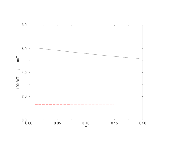
FIG. 1.: The full curve gives the inverse effective temperature $1/T^{*}=\beta m$ of the reference liquid as a function of the temperature $T$ in the glass phase. The Kauzman temperature is $T_{K}\simeq.194$. The dashed curves gives the square cage radius $A$ divided by the temperature and multiplied by $100$.

In fig. 1 we show the values of the inverse effective temperature ($1/T^{*}=\beta*m$) and of the square cage radius $A$, defined as $A={1\over 3}(\langle x_{i}^{2}\rangle-\langle x_{i}\rangle^{2})$. This square cage radius has been obtained by using in (7) as attractive potential: $w(r)=r^{2}/(4\beta S)$, and differentiating the free energy:

$$A={2\over d(m-1)N}\ {\partial(\beta F)\over\partial(1/S)}(S=\infty)$$ (22)

Notice that the effective temperature varies very little in the whole glass phase and remains close to the Kauzman temperature, while the square cage radius is nearly linear in temperature in the whole glass phase, which is natural since non harmonic effects have been neglected. The value of $A$ at the Kauzman temperature is $A\sim 2.5\ 10^{-3}$. This corresponds to a typical lateral displacement of the particle in each direction of order $\sqrt{A}\sim.05$, which is $.045$ of the mean interparticle distance, a value which gives the correct order of magnitude for the Lindeman ratio.

In fig. 2 we give the result for the specific heat in the glass phase versus the temperature. We see that it closely follows the Dulong-Petit law. This is the result that one should obtain since we study a solid phase in the classical framework. Notice that it is not at all trivial to derive this law from first principles in the glass phase. It is interesting to see it coming out naturally from our computations: although we are basically using the properties of the liquid at the effective temperature $T^{*}$, the fact that the optimal number of replicas $m$ vanishes linearly with $T$ at low temperatures naturally gives the Dulong-Petit law.

FIG. 2.: The internal energy (full line) and the specific heat (dashed line) of the glass versus the temperature derived from our analytic computation. The specific heat value is close to the Dulong-Petit value of 3/2 and reaches this value in the zero temperature limit.

From the knowledge of $F_{m}$ as a function of $m$, we can compute the configurational entropy as function of the free energy. In fig. 3 we plot the result for $\Sigma(f)$ versus $f$ at three different temperatures. We see that the curves are roughly parallel to each other, the main effect of the temperature changes being a shift in the $f$ axis.

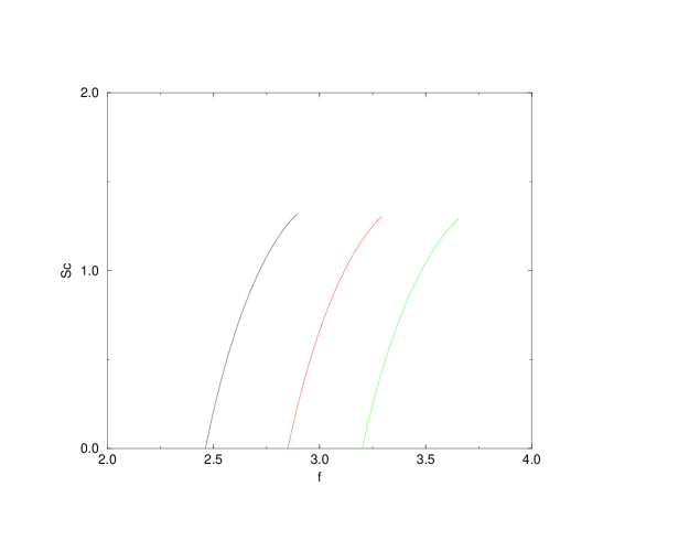
FIG. 3.: The configurational entropy $\Sigma(f)$ versus the free energy, computed analytically at temperatures $T=.05,.1,.15$, from right to left.

As discussed above (see (3)), the value of the configurational entropy at equilibrium is zero for $T<T_{K}$. It becomes non zero above $T_{K}$, where the saddle point in $m$ is at $m=1$. In fig. 4 we plot the equilibrium configurational entropy versus the temperature. It will be interesting to try to compare it with numerical simulations.

FIG. 4.: The equilibrium configurational entropy $\Sigma$ versus the temperature. It departs from zero above the Kauzman temperature.

To summarize, we have developed a well defined scheme for the analytic study of the thermodynamics of the glass phase. The basic knowledge one needs is the detailed properties of the liquid (particularly the instantaneous normal modes) close to the glass transition. We have shown that an implementation of this scheme with rather simple approximations leads to very reasonable results. We hope to be able to refine these approximations in a near future in order to get very precise predictions. The extension of this approach to dynamical properties is also a fascinating perspective.

- [1] E-mail: mezard@physique.ens.fr
- [2] E-mail: giorgio.parisi@roma1.infn.it
- [3] A recent review can be found in: C.A. Angell, Science, 267, 1924 (1995). See also G. Parisi, Proceedings of the ACS meeting, Orlando (1996), cond-mat/9701068, Lecture given at the Sitges conference, June 1996 cond-mat/9701034 and Lectures given at the Varenna summer school 1996, cond-mat/9705312.
- [4] G. Parisi Phys.Rev.Lett. 78(1997)4581
- [5] W. Kob and J.-L. Barrat, Phys.Rev.Lett. 79 (1997) 3660.
- [6] J.-L. Barrat and W. Kob, cond-mat/9806027.
- [7] S.Franz and G. Parisi, Phys. Rev. Letters (in press) and Effective potential in glassy systems: theory and simulations, cond-mat/9711215
- [8] B.Coluzzi and G.Parisi, cond-mat/9712261.
- [9] B. Bernu, Y. Hiwatari and J.P. Hansen, J.Phys. C18, L371 (1985); J.N. Roux, J.L. Barrat and J.P. Hansen,J.Phys. C1 7171 (1989).
- [10] A.W. Kauzman, Chem.Rev 43 (1948) 219.
- [11] G. Adams and J.H. Gibbs J.Chem.Phys 43 (1965) 139; J.H. Gibbs and E.A. Di Marzio, J.Chem.Phys. 28 (1958) 373.
- [12] T.R. Kirkpatrick and P.G. Wolynes, Phys. Rev. A34, 1045 (1986); T.R. Kirkpatrick and D. Thirumalai, Phys. Rev. Lett. 58, 2091 (1987); T.R. Kirkpatrick and D. Thirumalai, Phys. Rev. B36, 5388 (1987); T.R. Kirkpatrick, D. Thirumalai and P.G. Wolynes, Phys. Rev. A40, 1045 (1989).
- [13] D.J. Gross and M. Mézard, Nucl. Phys. B240 (1984) 431.
- [14] see for instance G.Parisi, cond-mat/9801034.
- [15] J.-P. Bouchaud and M. Mézard; J. Physique I (France) 4 (1994) 1109. E. Marinari, G. Parisi and F. Ritort; J. Phys. A27 (1994) 7615; J. Phys. A27 (1994) 7647.
- [16] J. Kurchan, G. Parisi, and M. A. Virasoro, J. Phys. I France 3, 1819 (1993).
- [17] A. Crisanti and H.-J. Sommers, J. Phys. I (France) 5, 805 (1995); A. Crisanti, H. Horner and H-J Sommers, Z.Phys. B 92, 257 (1993)
- [18] S. Franz, G. Parisi, J. Physique I 5 (1995) 1401.
- [19] R. Monasson, Phys. Rev. Lett. 75 (1995) 2847.
- [20] M.Cardenas, S. Franz and G. Parisi, cond-mat/99712099.
- [21] M .Mézard, G. Parisi and M.A. Virasoro, Spin glass theory and beyond, World Scientific (Singapore 1987).
- [22] For a review see W. Gotze, Liquid, freezing and the Glass transition, Les Houches (1989), J. P. Hansen, D. Levesque, J. Zinn-Justin editors, North Holland; C.A. Angell, Science, 267, 1924 (1995).
- [23] S. Franz and J. Hertz, Phys. Rev. Lett. 74, 2114 (1995).
- [24] J.-P. Bouchaud, L. Cugliandolo, J. Kurchan., M Mézard, Physica A 226, 243 (1996).
- [25] M.Mézard and G.Parisi, J. Phys. A 29 65155 (1996).
- [26] G.Toulouse, in ”Heidelberg colloquium on spin glasses”, I. Morgenstern and L. van Hemmen eds., Springer Verlag 1983.
- [27] S. Caracciolo, G. Parisi, S. Patarnello and N. Sourlas, Europhys. Lett. 11, 783 (1990).
- [28] M. Mézard and G. Parisi, in preparation.
- [29] See for instance T. Keyes, J.Phys.Chem. A 101 (1997) 2921, and references therein.
- [30] Y. Wan and R.M.Stratt, J.Chem.Phys. 100 (1994) 5123, and references therein.