Ab initio pseudopotentials for electronic structure calculations of poly-atomic systems using density-functional theory.

Abstract

The package fhi98PP allows one to generate norm-conserving pseudopotentials adapted to density-functional theory total-energy calculations for a multitude of elements throughout the periodic table, including first-row and transition metal elements. The package also facilitates a first assessment of the pseudopotentials’ transferability, either in semilocal or fully separable form, by means of simple tests carried out for the free atom. Various parameterizations of the local-density approximation and the generalized gradient approximation for exchange and correlation are implemented.

PROGRAM SUMMARY

Title of the program: fhi98PP
catalogue number: …
Program obtainable from: CPC Program Library, Queen’s University of Belfast, N. Ireland (see application form in this issue)
Licensing provisions: none
Computers on which the program has been developed: IBM/ RS 6000, Pentium PC
Operating system: UNIX
Graphics software to which output is tailored: XMGR or XVGR (both are public domain packages)
Programming language: FORTRAN 77
(non-standard feature is the use of END DO); UNIX C-shell scripts are employed as command line interfaces
Memory required to execute with typical data: $<$ 1 Mbyte
No. of bits in a word: 32
Memory required for test run: $<$ 1 Mbyte
Time for test run: $\approx$ 1 min
Number of lines in distributed program: 7500 (19000 with linear algebra library)
PACS codes: 71.15.Hx, 71.15.Mb, 71.15.-m, 82.20.Wt
Keywords: pseudopotential, total energy, electronic structure, density functional, local density, generalized gradient

Nature of the physical problem
The norm-conserving pseudopotential concept allows for efficient and accurate ab initio electronic structure calculations of poly-atomic systems. The key features of this approach are: (i) Only the valence states need to be calculated. The core states are considered as chemically inert, and removed within the frozen-core approximation. This exploits that many chemical and physical processes are governed by the valence states but only indirectly involve the core states. (ii) The valence electrons move in a pseudopotential which is much smoother than the true potential inside the small core regions around the nuclei, while reproducing it outside. This pseudopotential acts on smooth pseudo wavefunctions that are equivalent to the true valence wavefunctions, but avoid the radial nodes that keep the true valence and core orbitals orthogonal. This enables the use of computationally expedient basis sets like plane waves, and facilitates the numerical solution of the Schrödinger and Poisson equations in complicated systems. (iii) The norm-conservation constraint ensures that outside the core the pseudo wavefunctions behave like their all-electron counterparts over a wide range of different chemical situations. Along with a proper design, this makes the pseudopotential approach a dependable approximation in describing chemical bonds.

Derived and applied within density-functional theory [1, 2, 3], norm-conserving pseudopotentials [4, 5, 6] enable total-energy calculations of complex poly-atomic systems  [7, 8, 9] for a multitude of elements throughout the periodic table. Questions addressed with pseudopotentials provided by this code, or its earlier version, range from phase transitions [10, 11], defects in semiconductors [12, 13, 14], the structure of and diffusion on surfaces of semiconductors [15, 16, 17], simple metals [18], and transition metals [19, 20, 21], up to surface reactions [22, 23], including molecules [24, 25] of first-row species.

This package is a tool to generate and validate norm-conserving pseudopotentials, usable either in semilocal or in fully separable form, and including relativistic effects. Exchange and correlation is treated in the local-density approximation based on Ceperley and Alder’s data [26] as parametrized, e.g., by Perdew and Wang [27], or in the generalized gradient approximation, as proposed by Perdew, Burke, and Ernzerhof (PBE) [28], Perdew and Wang (PW91) [29], Becke and Perdew (BP) [30, 31], and by Lee, Yang, and Parr (BLYP) [32].

Method of solution
The first part of the program (psgen) generates pseudopotentials of the Hamann [33] or the Troullier-Martins type [34], based on a scalar-relativistic all-electron calculation of the free atom. A partial core density can be included to allow for nonlinear core-valence exchange-correlation [35] where needed, e.g., for spin-density functional calculations, alkali metal compounds, and the cations of II-VI compounds like ZnSe. The second part (pswatch) serves to assess the transferability of the pseudopotentials, examining scattering properties, excitation energies, and chemical hardness properties of the free pseudo atom. Transcribing the pseudopotentials into the fully separable form of Kleinman and Bylander [36], we verify the absence of unphysical states by inspection of the bound state spectrum and by the analysis of Gonze et al. [37]. The convergence of the pseudo wavefunctions in momentum space is monitored in order to estimate a suitable basis set cutoff in plane wave calculations.

Restrictions on the complexity of the problem
(i) Only some of the GGA’s currently in use are implemented, others may be readily added however. (ii) The present pseudopotentials yield the correct relativistic valence levels where spin-orbit splittings are averaged over, as it is intended for most applications.

1 Introduction

Electronic structure and total-energy calculations using density-functional theory [1, 2, 3] have grown into a powerful theoretical tool to gain a quantitative understanding of the physics and chemistry of complex molecular, liquid, and solid state systems. The norm-conserving pseudopotential approach provides an effective and reliable means for performing such calculations in a wide variety of poly-atomic systems, particularly, though not only, together with a plane wave basis and modern minimization algorithms for the variational determination of the ground state [7, 8, 9, 38]. In this approach only the chemically active valence electrons are dealt with explicitly. The chemically inert core electrons are eliminated within the frozen-core approximation [39], being considered together with the nuclei as rigid non-polarizeable ion cores. In turn, all electrostatic and quantum-mechanical interactions of the valence electrons with the ion cores (the nuclear Coulomb attraction screened by the core electrons, Pauli repulsion and exchange-correlation between core and valence electrons) are accounted for by angular momentum dependent pseudopotentials. These reproduce the true potential and valence orbitals outside a chosen core region but remain much weaker inside. The valence electrons are described by smooth pseudo orbitals which play the same role as the true orbitals, but avoid the nodal structure near the nuclei that keeps core and valence states orthogonal in an all-electron framework. The respective Pauli repulsion largely cancels the attractive parts of the true potential in the core region, and is built into the therefore rather weak pseudopotential [40]. This “pseudoization” of the valence wavefunctions along with the removal of the core states eminently facilitates a numerically accurate solution of the Schrödinger and Poisson equations, and enables the use of plane waves as an expedient basis set in electronic structure calculations. By virtue of the norm-conserving property [4, 5] and when constructed properly pseudopotentials present a rather marginal approximation, and indeed allow for an adequate description of the valence electrons over the entire chemically relevant range of systems, i.e. atoms, molecules, and solids.

Here we supply a two-piece package to generate norm-conserving pseudopotentials adapted to density-functional electronic structure calculations, and usable in semilocal or fully separable form. Generic input files for many elements are distributed along with the package.

Part 1 (program psgen) serves to generate the pseudopotentials using the schemes by Hamann [33] or by Troullier and Martins [34]. This combination provides efficient pseudopotentials for “canonical” applications like group IV and III-V semiconductors [9, 10, 15, 16, 17, 22, 23], as well as for systems where first-row, transition or noble metal elements are present [11, 19, 20, 21, 24, 25], or where “semicore” $d$-states must be treated as valence states, like in GaN [41] or InN [14]. In such cases the strongly localized $2p$ and $3,4,5d$ valence states are readily handled with the Troullier-Martins scheme. Both schemes have been routinely employed and have an established track record with the electronic structure and ab initio molecular dynamics package fhi96md [9]. The pseudopotentials are derived within density-functional theory, starting from a scalar-relativistic all-electron calculation of the free atom [42]. Accordingly they yield the proper relativistic positions of the valence levels [43] with the spin-orbit coupling being averaged over, in line with the practice in most applications. The exchange-correlation interaction may be described within the local-density approximation (LDA) [44, 45], or the generalized gradient approximation (GGA) [46]. For the LDA, the package includes the expressions by Perdew and Wang [27], and by Perdew and Zunger [47], both parameterizing Ceperley and Alder’s results for the homogeneous electron gas [26]. Earlier prescriptions by Hedin and Lundquist [48], and Wigner [49] are supplied as well. For the GGA, the package includes the formulations by Perdew, Burke, and Ernzerhof (PBE) [28], by Perdew and Wang (PW91) [29], as well as those composed from the exchange functional by Becke [30] (or that of Ref. [29]) and the correlation functional either by Perdew (BP) [31], or by Lee, Yang, and Parr (BLYP) [32]. Alternative forms can be readily added to the code. Hence the pseudopotentials, i.e. the electron-ion interaction, can be generated consistently using the same exchange-correlation scheme as for calculating the poly-atomic system [50]. A partial core density may be included in the unscreening of the pseudopotentials to explicitly account for the nonlinearity of core-valence exchange-correlation of the above functionals [35]. This has proven necessary, e.g., for alkali metal elements [51], the cations in strongly polar compounds like ZnSe [52], or calculations of spin-polarized systems [53].

Part 2 (program pswatch) facilitates the assessment of the pseudopotentials’ transferability, that is, their proper performance in different chemical environments. This is done for the free (pseudo) atom by checking that its scattering properties, excitation energies and chemical hardness properties [54, 55] faithfully represent those of the corresponding all-electron atom. For this purpose, we evaluate the logarithmic derivatives of the valence wavefunctions, total energies and orbital eigenvalues for different valence configurations. For the commonly used fully separable Kleinman-Bylander form of the pseudopotentials [36], it is important to rule out “ghost states”, i.e. unphysical bound states or resonances appearing in the valence spectrum. As an immediate check we evaluate the bound state spectrum of the fully separable potentials, and apply the analysis by Gonze et al. [37]. To assess the convergence behavior of the pseudopotentials we monitor the pseudo atom’s kinetic energy in momentum space [56], which also allows a first estimate of a suitable basis cutoff for plane wave calculations.

In Chapter 2 of this Communication we briefly survey the conceptual aspects of constructing and validating pseudopotentials, more practical topics being addressed towards the end of a section. Chapter 3 is meant as a reference guide to our package.

2 General background and formalism

A pseudopotential is constructed to replace the atomic all-electron potential such that core states are eliminated and the valence electrons are described by nodeless pseudo wavefunctions. In doing so the principal objectives to consider are (i) the transferability of the pseudopotential, its ability to accurately describe the valence electrons in different atomic, molecular, and solid-state environments. In self-consistent total energy calculations this means that the valence states have the proper energies and lead to a properly normalized electron distribution which in turn yields proper electrostatic and exchange-correlation potentials, particularly outside the core region, i.e. where chemical bonds build up. (ii) their efficiency, that is to keep the computational workload in applications as low as possible, allowing to compute wavefunctions and electron densities with as few basis functions (being “soft”) and operations as possible. Modern norm-conserving pseudopotentials, implemented here in the variants proposed by Hamann [33] and by Troullier-Martins [34], allow for a controlled “compromise” with respect to these (conflicting) tasks, through appropriate choices and tests at several stages of their actual construction.

Norm-conserving pseudopotentials are derived from an atomic reference state (Sec. 2.1 and 2.2), requiring that the pseudo and the all-electron valence eigenstates have the same (reference) energies and the same amplitude (and thus density) outside a chosen core cutoff radius $r^{c}$. Normalizing the pseudo orbitals then implies that they include the same amount of charge in the core region as their all-electron counterparts, being “norm-conserving”. At the reference energies, the pseudo and all-electron logarithmic derivatives (which play the role of boundary conditions on the wavefunctions inside and outside the core region) agree for $r\geq r^{c}$ by construction. Norm-conservation then ensures that the pseudo and all-electron logarithmic derivatives agree also around each reference level, to first order in the energy, by virtue of the identity

$$-\frac{1}{2}r^{2}|\psi(\epsilon;{\bf r})|^{2}\frac{d}{d\epsilon}\left\{\frac{d}{dr}\ln\psi(\epsilon;{\bf r})\right\}\Bigg{|}_{\,{}^{\scriptstyle r=r^{\rm c}}_{\scriptstyle\epsilon=\epsilon^{\prime}}}=\int\!\!\int_{0}^{r^{c}}|\psi(\epsilon^{\prime};{\bf r})|^{2}r^{2}dr\,d\Omega\quad,$$ (1)

where $\psi(\epsilon;{\bf r})$ denotes the regular solution of the Schrödinger equation at some energy $\epsilon$ (not necessarily an eigenfunction) for either the all-electron potential or the pseudopotential. A norm-conserving pseudopotential thus exhibits the same scattering properties (logarithmic derivatives) as the all-electron potential in the neighborhood of the atomic eigenvalues, typically it does so over the entire energy range of valence bands or molecular orbitals, which is an important prerequisite and measure for the pseudopotential’s proper performance.

Regarding transferability the quality of a pseudopotential depends on (a) correct scattering properties, (b) the actual choice of the core cutoff radius $r^{c}$, larger values leading to softer pseudopotentials (more rapidly convergent in say plane wave calculations) but tending to decrease their accuracy, as the pseudo wavefunctions and the pseudopotential begin to deviate from their true counterparts even at radii that are relevant to bonding, (c) an adequate account of the nonlinear exchange-correlation interaction between core and valence electrons (Sec. 2.3), which is often treated linearly through the pseudopotential and thus approximated, (d) if applied, the quality of the Kleinman-Bylander form of the pseudopotential, where accidental spurious states need to be avoided (Sec. 2.6), (e) the validity of the frozen-core approximation, i.e. the inclusion of all relevant states as valence states which may include upper semicore states in addition to the outermost atomic shell, dependent on the actual chemical context, say, if these hybridize with valence states of neighboring atoms (Sec. 2.3), and (f) the treatment of higher angular momentum components which are just implicitly considered in the pseudopotential’s construction (Sec. 2.5). As outlined in Sec. 2.4 the points (a) – (e) can be controlled with respect to transferability by verifying that the pseudo atom reproduces the all-electron atom’s scattering properties and excited states. The latter essentially probe the atom’s response or hardness properties due to a change in the occupation of the valence orbitals [54]. Such tests for the free atom are less conclusive for (e) and (f) which, though mostly uncritical, should be kept in mind as potential sources of pseudopotential errors in poly-atomic systems.

Usually norm-conserving pseudopotentials are set up and derived in terms of an angular momentum dependent, “semilocal” operator,

$$\langle{\bf r}|\hat{V}^{\rm ps}|{\bf r}^{\prime}\rangle=V^{\rm loc}(r)\delta({\bf r}-{\bf r}^{\prime})+\sum_{l=0}^{l_{\rm max}}\sum_{m=-l}^{m=l}Y^{*}_{lm}(\Omega_{{\bf r}})\delta V^{\rm ps}_{l}(r)\frac{\delta(r-r^{\prime})}{r^{2}}Y_{lm}(\Omega_{{\bf r}^{\prime}})\quad,$$ (2)

written in terms of a local pseudopotential $V^{\rm loc}(r)$, and $l$-dependent components $\delta V^{\rm ps}_{l}(r)=V^{\rm ps}_{l}(r)-V^{\rm loc}(r)$ which are confined to the core region and eventually vanish beyond some $l_{\rm max}$ (see Sec. 2.5). For reasons of computational efficiency the semilocal form is often transcribed into the fully nonlocal Kleinman-Bylander form [36] (Sec. 2.6). Relativistic effects on the electrons, important for heavier elements, basically originate just in the core region. Whence they may be incorporated in the pseudopotentials [57, 58] which we do here within a scalar-relativistic approximation (Sec. 2.1). Accordingly, such “relativistic” pseudopotentials are formally employed with a non-relativistic Schrödinger equation.

The next subsections discuss the construction of this package’s pseudopotentials, which in short proceeds as follows,

• Density-functional calculation of the all-electron atom in a reference state (ground state), within a scalar-relativistic framework and a chosen approximation for exchange-correlation (Sec. 2.1).

• Construction of the pseudo valence orbitals and (screened) pseudopotential components, observing the norm-conserving constraints (Sec. 2.2).

• Removal of the electrostatic and exchange-correlation components due to the valence electrons from the screened pseudopotential, optionally taking nonlinear core-valence effects into account. This “unscreening” yields the ionic pseudopotential representing the electron-ion interaction in poly-atomic systems (Sec. 2.3).

• Assessment of the pseudopotential’s transferability (Sec. 2.4), in case of a transformation to the fully separable Kleinman-Bylander form the exclusion of unphysical “ghost states” in the valence spectrum (Sec. 2.6).

Hartree atomic units are used throughout ($e^{2}=\hbar=m=1$), lengths being given in units of the Bohr radius $1\,\mbox{bohr}=0.52918\,\mbox{\AA}$, and energies in units of $1\,\mbox{hartree}=27.2116\,\mbox{eV}$.

2.1 Atomic all-electron calculation

The initial step in constructing our pseudopotentials is an all-electron calculation of the free atom in a reference configuration, usually its neutral ground-state. Using density-functional theory to handle the many-electron interactions, the total energy of $N$ electrons in an external potential $V^{\rm ext}({\bf r})$ (for an atom the nuclear $-Z/r$ potential) is written as a functional of the electron density $\rho$,

$$E^{\rm tot}[\rho]=T[\rho]+E^{\rm XC}[\rho]+E^{\rm H}[\rho]+\int-\frac{Z}{r}\rho({\bf r})d^{3}r\quad,$$ (3)

where $T[\rho]$ is the non-interacting kinetic energy, $E^{\rm XC}[\rho]$ the exchange and correlation energy, and $E^{\rm H}[\rho]=\frac{1}{2}\int\frac{\rho({\bf r})\rho({\bf r}^{\prime})}{|{\bf r}-{\bf r}^{\prime}|}d^{3}r\,d^{3}r^{\prime}$ the electrostatic or Hartree energy from the electron-electron repulsion. The ground-state corresponds to the minimum of $E^{\rm tot}[\rho]$, and is found from the self-consistent solution of the Kohn-Sham equations

$$\left[-\frac{1}{2}\nabla^{2}+V^{\rm eff}[\rho;{\bf r}]-\epsilon_{i}\right]\psi_{i}({\bf r})=0\quad,$$ (4)

$$V^{\rm eff}[\rho;{\bf r}]=\int\frac{\rho({\bf r})}{|{\bf r}-{\bf r}^{\prime}|}d^{3}r+\frac{\delta E^{\rm XC}[\rho]}{\delta\rho({\bf r})}+V^{\rm ext}({\bf r})\quad,$$ (5)

$$\rho({\bf r})=\sum_{i}f_{i}|\psi_{i}({\bf r})|^{2}\quad,\quad\int\rho({\bf r})d^{3}r=N\quad,$$ (6)

$$f_{i}=1\quad\mbox{if}\quad\epsilon_{i}\leq\epsilon_{N}\quad,\,\,0\leq f_{i}\leq 1\quad\mbox{if}\quad\epsilon_{i}=\epsilon_{N}\quad,\,\,\mbox{ and}\quad f_{i}=0\quad\mbox{if}\quad\epsilon_{i}>\epsilon_{N}\quad.$$ (7)

Specializing to a spherically symmetric electron density and effective potential the Kohn-Sham orbitals separate, $\psi_{i}({\bf r})=[u_{n_{i}l_{i}}(\epsilon_{i};r)/r]Y_{l_{i}m_{i}}(\Omega_{{\bf r}})$ and (4) reduces to a radial Schrödinger equation. Relativistic effects, which in principle require a four-current and Dirac-spinor formulation of Eqs. (3) – (7), are treated by using a scalar-relativistic kinetic energy operator [42]. This takes into account the kinematic relativistic terms (the mass-velocity and Darwin terms) needed to properly describe the core states and the relativistic shifts of the valence levels, in particular for the heavier elements. The spin-orbit coupling terms are averaged over, as is commonly done in most applications (see also Ref. [58]). The radial wavefunctions $u_{nl}$ are then the self-consistent eigenfunctions of the scalar-relativistic Schrödinger equation

$$\left[\frac{1}{2M(r)}\left(-\frac{d^{2}}{d\,r^{2}}-\frac{1}{2M(r)c^{2}}\frac{d\,V(r)}{d\,r}r\frac{d}{d\,r}\frac{1}{r}+\frac{l(l+1)}{r^{2}}\right)+V(r)-\epsilon_{i}\right]u_{nl}(\epsilon_{i};r)=0\,\,,$$ (8)

with the relativistic electron mass $M(r)=1+\frac{\epsilon_{i}-V(r)}{2c^{2}}$, where $1/c=1/137.036$ is the finestructure constant, the effective all-electron potential

$$V(r)=V^{\rm XC}[\rho;r]+V^{\rm H}[\rho;r]-\frac{Z}{r}\quad,$$ (9)

the exchange-correlation potential $V^{\rm XC}[\rho;r]=\frac{\delta E^{\rm XC}[\rho]}{\delta\rho(r)}$  , and the Hartree potential

$$V^{\rm H}[\rho;r]=\frac{\delta E^{\rm H}[\rho]}{\delta\rho(r)}=4\pi\frac{1}{r}\int_{0}^{r}\rho(r^{\prime}){r^{\prime}}^{2}dr^{\prime}+4\pi\int_{r}^{\infty}\rho(r^{\prime})r^{\prime}dr^{\prime}\quad.$$ (10)

Due to the spherical symmetry, states with the same quantum numbers $n_{i}=n$ and $l_{i}=l$ , but different $m_{i}$ are energetically degenerate, $\epsilon_{i}=\epsilon_{n_{i}l_{i}m_{i}}=\epsilon_{nl}$, and therefore equally occupied by $0\leq f_{i}\leq f_{nl}/(2l+1)$ electrons, where the occupancies $f_{nl}$ stand for the total number of electrons in the $nl$-shell. This leads to the electron density

$$\rho(r)=\frac{1}{4\pi}\sum_{n=1}\sum_{l=0}^{n-1}f_{nl}\left|\frac{u_{nl}(\epsilon_{nl};r)}{r}\right|^{2}\,\,,\mbox{with}\quad\left\{\begin{array}[]{cl}f_{nl}=2(2l+1)&\mbox{for}\quad\epsilon_{nl}<\epsilon_{N}\,,\\ 0\leq f_{nl}\leq 2(2l+1)&\mbox{for}\quad\epsilon_{nl}=\epsilon_{N}\,,\\ f_{nl}=0&\mbox{for}\quad\epsilon_{nl}>\epsilon_{N}\,,\end{array}\right.$$ (11)

with the total number of electrons being $\sum_{nl}f_{nl}=N\,$. The non-relativistic Kohn-Sham equations are recovered by setting the finestructure constant $1/c$ in Eq. (8) to zero. The above scheme determines the atomic ground state. Excited atomic states are calculated with appropriately specified occupancies (as usual, we treat the occupancies always as parameters, a database of ground state configurations $\{f_{nl}\}$ being supplied with this package).

Regarding exchange-correlation, the program allows to employ commonly used parameterizations of the local-density approximation (LDA) and of the generalized gradient approximation (GGA). In the LDA the exchange-correlation energy is

$$E^{\rm XC-LDA}[\rho]=\int\rho(r)\,\varepsilon^{\rm XC-LDA}(\rho(r))d^{3}r\quad,$$ (12)

where $\varepsilon^{\rm XC-LDA}(\rho)=\varepsilon^{\rm X-LDA}(\rho)+\varepsilon^{\rm C-LDA}(\rho)$ represents the exchange-correlation energy per electron of a uniform electron gas. Its exchange part reads $\varepsilon^{\rm X-LDA}(\rho)=-\frac{3}{4\pi}(3\pi^{2}\rho)^{1/3}$. For the correlation part $\varepsilon^{\rm C-LDA}(\rho)$ representations given by Perdew and Wang [29] and, previously, by Perdew and Zunger [47] may be used. Both are parameterizations of Ceperley and Alder’s exact results for the uniform electron gas [26]. To facilitate comparisons with results in the existing literature, we also supply the earlier prescriptions by Hedin and Lundquist [48], and by Wigner [49]. For an overview of the LDA we refer to Ref. [45]. These (nonrelativistic) LDA exchange-correlation functionals may be supplemented with relativistic corrections to the exchange part, as given by MacDonald and Vosko [59, 60]. The LDA exchange-correlation potential is given by

$$V^{\rm XC-LDA}[\rho;r]=\left[1+\rho(r)\frac{d}{d\rho}\right]\varepsilon^{\rm XC-LDA}(\rho(r))\quad.$$ (13)

In a GGA the exchange-correlation functional depends on the density and its gradient,

$$E^{\rm XC-GGA}[\rho]=\int\rho(r)\varepsilon^{\rm XC-GGA}(\rho(r),|\nabla\rho(r)|)\,d^{3}r\quad.$$ (14)

This code includes the GGA functionals by Perdew and Wang (PW91) [29], by Perdew, Burke, and Ernzerhof (PBE) [28], and Becke’s formula for the exchange part [30] combined with Perdew’s 1986 formula for correlation [31] (BP). Substituting for the latter the formula of Lee, Yang, and Parr (LYP) [32] provides the so-called BLYP GGA. Relativistic corrections to the GGA as proposed by Engel et al.  [61] are not included here. The GGA exchange-correlation potential (in cartesian coordinates) is given by

$$V^{\rm XC-GGA}[\rho;r]=\left[\frac{\partial}{\partial\rho}-\sum_{i=1}^{3}\nabla_{i}\frac{\partial}{\partial\nabla_{i}\rho}\right]\rho(r)\varepsilon^{\rm XC-GGA}(\rho(r),|\nabla\rho(r)|)\quad,$$ (15)

and depends on the first and second radial derivatives of the density. It is an open issue whether to prefer one of these GGAs over another. Dependent on the application, they may yield somewhat differing results. However, the actual choice among these GGAs is usually less important than the differences between the LDA and the GGAs themselves. A discussion of the various GGAs can be found in Ref. [46].

Whether to use either the LDA or the GGA in constructing pseudopotentials is determined by the exchange-correlation scheme one wants to use for the poly-atomic system. If using the GGA there, the pseudopotential should be generated within the (same) GGA rather than the LDA, in order to describe the exchange-correlation contribution to the core-valence interactions within the GGA too. This “consistent” use of the GGA may be significant to resolve any differences between LDA and GGA properly, i.e. to the same extent as with all-electron methods [50] (see also Sec. 2.3).

2.2 Screened norm-conserving pseudopotentials

Having obtained the all-electron potential and valence states, we use either the scheme by Hamann [33], or by Troullier and Martins [34] to construct the intermediate, so called screened pseudopotential. The latter acts as the effective potential on the (pseudo) valence states $\psi^{\rm ps}_{lm}({\bf r})=\left[u^{\rm ps}_{l}(\epsilon^{\rm ps}_{l};r)/r\right]Y_{lm}(\Omega_{{\bf r}})$, where the radial part for the angular momentum $l$ is the lowest eigenfunction of the nonrelativistic Schrödinger equation,

$$\left[-\frac{1}{2}\frac{d^{2}}{dr^{2}}+\frac{l(l+1)}{2r^{2}}+V^{\rm ps,scr}_{l}(r)-\epsilon^{\rm ps}_{l}\right]u^{\rm ps}_{l}(\epsilon^{\rm ps}_{l};r)=0\quad.$$ (16)

Initially, a radial pseudo wavefunction $u^{\rm ps}_{l}(r)$ is derived from the all-electron valence level with angular momentum $l$ (the reference level [62]) such that

1. The pseudo wavefunction and the all-electron wavefunction correspond to the same eigenvalue

   $$\epsilon^{\rm ps}_{l}\equiv\epsilon_{nl}\quad,$$ (17)

   and their logarithmic derivatives (and thus the respective potentials) agree beyond a chosen core cutoff radius $r^{\rm c}_{l}$,

   $$\frac{d}{dr}\ln u^{\rm ps}_{l}(\epsilon^{\rm ps}_{l};r)\rightarrow\frac{d}{dr}\ln u_{nl}(\epsilon_{nl};r)\quad\mbox{for}\quad r>r^{\rm c}_{l}\quad.$$ (18)

2. The radial pseudo wavefunction has the same amplitude as the all-electron wavefunction beyond the core cutoff radius,

   $$u^{\rm ps}_{l}(\epsilon^{\rm ps}_{l};r)\rightarrow u_{nl}(\epsilon_{nl};r)\quad\mbox{for}\quad r>r^{\rm c}_{l}\quad,$$ (19)

   and is normalized, $\int_{0}^{\infty}|u^{\rm ps}_{l}(\epsilon^{\rm ps}_{l};r)|^{2}dr=\int_{0}^{\infty}|u_{nl}(\epsilon_{nl};r)|^{2}dr=1$. This implies the norm-conservation constraint

   $$\int_{0}^{r^{\prime}}|u^{\rm ps}_{l}(\epsilon^{\rm ps}_{l};r)|^{2}dr\equiv\int_{0}^{r^{\prime}}|u_{nl}(\epsilon_{nl};r)|^{2}dr\quad\mbox{, for}\quad r^{\prime}\geq r^{\rm c}_{l}\quad.$$ (20)

3. The pseudo wavefunction contains no radial nodes. In order to obtain a continuous pseudopotential which is regular at the origin, it is twice differentiable and satisfies $lim_{r\rightarrow 0}u^{\rm ps}_{l}(r)\propto r^{l+1}$.

The pseudopotential components then correspond to an inversion of the Schrödinger equation (16) for the respective pseudo wavefunctions,

$$V^{\rm ps,scr}_{l}(r)=\epsilon^{\rm ps}_{l}-\frac{l(l+1)}{2r^{2}}+\frac{1}{2u^{\rm ps}_{l}(r)}\frac{d^{2}}{d\,r^{2}}u^{\rm ps}_{l}(r)\quad.$$ (21)

and become identical to the all-electron potential beyond $r\geq r^{\rm c}_{l}$.

The ansatz for the spatial function $u^{\rm ps}_{l}(r)$ at the energy $\epsilon^{\rm ps}_{l}$ requires three free parameters to meet the constraints (i) and (ii). The Hamann scheme is of this “minimal” type, while the Troullier-Martins scheme introduces additional constraints, namely that the pseudopotential’s curvature vanish at the origin, $\frac{d^{2}}{dr^{2}}V^{\rm ps,scr}_{l}(r)|_{r=0}=0$, and that all first four derivatives of the pseudo and the all-electron wavefunction agree at the core cutoff radius. Thereby it achieves softer pseudopotentials for the $2p$, and the $3,4,5d$ valence states of the first row, and of the transition metal elements, respectively. For other elements both schemes perform rather alike. We refer to the original references [33] and [34] for the details about the construction procedure. Here we point out that both schemes technically differ somewhat regarding the radii where the pseudo wavefunctions and pseudopotentials match their all-electron counterparts. The Hamann scheme accomplishes the matching exponentially beyond the core cutoff radius $r^{\rm c-H}_{l}$, while in the Troullier-Martins scheme this matching is exact at and beyond $r^{\rm c-TM}_{l}$. Although in the Hamann scheme the core cutoff radii are nominally smaller, $r^{\rm c-H}_{l}/r^{\rm c-TM}_{l}\approx 0.25\ldots 0.75$, the pseudo wavefunctions and pseudopotentials converge to the all-electron wavefunctions and potential within a similar range as in the Troullier-Martins scheme.

Default values for the core cutoff radii are provided by the program psgen. In the Hamann case it determines the position $r^{\rm Max}_{l}$ of the outermost maximum of the all-electron wavefunction and sets $r^{\rm c-H}_{l}=0.6\,r^{\rm Max}_{l}$ if there are core states present with the same angular momentum, and to $r^{\rm c-H}_{l}=0.4\,r^{\rm Max}_{l}$ otherwise [33]. In the Troullier-Martins case the core cutoff radii are set to values which we have tabulated for all elements up to Ag (except the lanthanides). Except for some finetuning that might be necessary when the pseudopotentials are used in the Kleinman-Bylander form (see Sec. 2.6) these default values should yield a reasonable compromise between pseudopotential transferability and efficiency.

In general, increasing $r^{\rm c}_{l}$ yields softer pseudopotentials, which converge more rapidly e.g. in a plane wave basis. These will become less transferable however as the pseudo wavefunctions become less accurate at radii relevant to bonding. When decreasing $r^{\rm c}_{l}$ one has to keep in mind that $r^{\rm c}_{l}$ has to be larger than the radius of the outermost radial node in the respective all-electron orbital. Taking $r^{\rm c}_{l}$ too close to such a node results in poor pseudopotentials, as it is essentially at variance with requiring both a nodeless and at the same time norm-conserving pseudo wavefunction. A rugged or multiple-well structure seen in a plot of the screened pseudopotential and poor scattering properties (see Sec. 2.4) can indicate such a breakdown.

Treating components without bound reference states

So far we have considered pseudopotentials for bound reference states. On the other hand it is quite common in LDA and GGA that unoccupied states in the neutral atom are not or only weakly bound, for instance the $3d$-wavefunctions for Al, Si, etc. . To derive a $l$-component of the pseudopotential in such cases we follow the generalized norm-conserving procedure proposed by Hamann [33]: At a chosen energy $\epsilon_{l}$ the Schrödinger equations for the all-electron potential and the pseudopotential are integrated from the origin up to a matching radius $r^{\rm match}_{l}$. There the logarithmic derivatives and the amplitudes of the pseudo and all-electron partial waves are matched, and the “normalization” $\int_{0}^{r^{\rm match}_{l}}|u^{\rm ps}_{l}(\epsilon_{l};r)|^{2}dr=\int_{0}^{r^{\rm match}_{l}}|u_{nl}(\epsilon_{l};r)|^{2}dr\,:=\,1$ is enforced. This procedure is analogous to (17) – (20) for bound states. The corresponding pseudopotential component results from (21), and merges into the all-electron potential for $r>r^{\rm match}_{l}$. The value of $\epsilon_{l}$ should be chosen in the energy range where the valence states are expected to form bands or molecular orbitals, as a default, the program psgen employs the highest eigenvalue of the occupied states, e.g., for Al to $\epsilon_{l=2}=\epsilon_{3p}$. Hamann’s procedure for unbound states is not tied to a particular type of pseudopotential, we use it in constructing Troullier-Martins as well as Hamann pseudopotential functions. Figure 1 displays the Hamann-type pseudo wavefunctions and pseudopotential components for aluminum. Alternatively, one can derive the $l$-components without bound states in the neutral atom from a (separate) calculation of an ionized or excited atom which supports bound states for these $l$’s [6]. The above prescriptions should both yield rather similar pseudopotentials, consistent with the supposition that pseudopotentials are transferable among neutral and excited atomic states.

2.3 Ionic pseudopotentials, unscreening, and nonlinear core-valence exchange-correlation

The final ionic pseudopotentials are determined by subtracting from the screened pseudopotentials the electrostatic and the exchange-correlation screening contributions due to the valence electrons,

$$V^{\rm ps}_{l}(r)=V^{\rm ps,scr}_{l}(r)-V^{\rm H}[\rho^{\rm ps}_{0};r]-V^{\rm XC}[\rho^{\rm ps}_{0};r]\quad\mbox{with}\quad\rho^{\rm ps}_{0}(r)=\frac{1}{4\pi}\sum_{l=0}f_{l}\left|\frac{u^{\rm ps}_{l}(\epsilon^{\rm ps}_{l};r)}{r}\right|^{2}\quad.$$ (22)

The valence electron density is evaluated from the atomic pseudo wavefunctions, with the same occupancies $f_{l}$ as for the all-electron valence states of Sec. 2.1. Figure 1 shows the ionic pseudopotentials for aluminum as an example. With the pseudopotentials as defined by Eq. (22) the electronic total energy of an arbitrary system reads

$$E^{\rm tot}=\sum_{i}f_{i}\langle\psi_{i}|\hat{T}+\hat{V}^{\rm ps}|\psi_{i}\rangle+E^{H}[\rho^{\rm ps}]+E^{\rm XC}[\rho^{\rm ps}]\quad\mbox{with}\quad\rho^{\rm ps}({\bf r})=\sum_{i}f_{i}|\psi_{i}({\bf r})|^{2}\quad.$$ (23)

Figure 1: Graphical output from psgen for aluminum. The left panel shows the valence wavefunctions for the pseudo atom (solid lines) and the all-electron atom (dashed). The right panel shows the respective Hamann-type ionic pseudopotential, using Hamann’s procedure to treat the $d$-component (see Sec. 2.2) and the LDA. The legends give the core cutoff radii $r^{\rm c}_{l}$ (in bohr).

Here, $E^{\rm XC}$ refers to the exchange-correlation interaction between the valence electrons themselves. That between the valence and the core electrons is included in the pseudopotential energy, as a term which depends linearly on the valence density $\rho^{\rm ps}$. Although $E^{\rm XC}$ is a nonlinear functional of the total electron density $\rho$, the above “linearization” of its core-valence contribution is a usual and mostly adequate approximation for calculations within both LDA and GGA [50]. However, an explicit account of the core-valence nonlinearity of $E^{\rm XC}$ is sometimes required, for instance in studies involving alkali metal atoms or within spin-density functional theory. This is accomplished by restoring the dependence of $E^{\rm XC}$ (and $V^{\rm XC}$) on the total electron density, i.e. adding the (atomic) core density to the valence density in the argument of $E^{\rm XC}$. In turn the ionic pseudopotentials (22) are redefined. Rather than the full core density, it suffices to add a so called partial core density $\tilde{\rho}^{\rm core}_{0}$, as suggested by Louie et al. [35]. It reproduces the full core density $\rho^{\rm core}_{0}$ (47) outside a chosen cutoff radius $r^{\rm nlc}$ but is a smoother function inside, which enables its later use together with plane waves. We use a polynomial

$$\tilde{\rho}^{\rm core}_{0}(r)=\left\{\begin{array}[]{lll}\rho^{\rm core}_{0}(r)&\mbox{for}&\quad r\geq r^{\rm nlc}\,\,,\\ c_{0}+\sum_{i=3}^{6}c_{i}r^{i}&\mbox{for}&\quad r<r^{\rm nlc}\,\,,\mbox{with}\quad\tilde{\rho}^{\rm core}_{0}(r)<\rho^{\rm core}_{0}(r)\quad,\end{array}\right.$$ (24)

where we take the coefficients $c_{i}$ such that $\tilde{\rho}^{\rm core}_{0}(r)$ has zero slope and curvature at the origin, decays monotonically, and joins the full core density continuously up to the third derivative. In this way smooth exchange-correlation potentials result for the LDA as well as for the GGAs. The resulting nonlinear core-valence exchange-correlation scheme uses the redefined ionic pseudopotentials

$$V^{\rm ps}_{l}(r)\rightarrow V^{\rm ps,scr}_{l}(r)-V^{\rm H}[\rho^{\rm ps}_{0};r]-V^{\rm XC}[\rho^{\rm ps}_{0}+\tilde{\rho}^{\rm core}_{0};r]\quad$$ (25)

instead of Eq. (22). The according total energy expression is

$$E^{\rm tot}\rightarrow\sum_{i}f_{i}\langle\psi_{i}|\hat{T}+\hat{V}^{\rm ps}|\psi_{i}\rangle+E^{H}[\rho^{\rm ps}]+E^{\rm XC}[\rho^{\rm ps}+\tilde{\rho}^{\rm core}_{0}]\quad,$$ (26)

where, in a poly-atomic system, $\tilde{\rho}^{\rm core}_{0}$ stands for the superimposed partial core densities of the constituent atoms.

Whether nonlinear exchange-correlation plays a significant role can be readily decided by a comparison of two calculations with and without a partial core density. As a rule, it becomes more important to the left in the periodic table, i.e. with fewer electrons in the valence shell (alkali metals), and with increasing atomic number, i.e. the farther the upper core orbitals extend into the tail of the valence density (e.g. Zn, Cd). Of course if the uppermost semicore states hybridize with “true” valence states they have to be treated as valence states in the first place, like the $3,4,5d$-states in all transition and noble metals, but also the $3d$-states in Ca. This also applies for the $3d$- and $4d$-states of Ga and In in GaN and InN, where these interact markedly with the N atoms’ $2s$-states in GaN and InN, while treating them in the core is indeed adequate in, say, GaAs or InAs.

There remains the question what value to pick for the core cutoff radius $r^{\rm nlc}$. It is reasonable to set $r^{\rm nlc}$ to about the radius where the full core density drops below the valence electron density. The utility psgen determines this “equi-density radius” and also outputs the core and valence densities. Choosing $r^{\rm nlc}$ smaller makes it more demanding to represent the partial core, say, in a plane wave basis, without further enhancing the pseudopotential’s performance. On the other hand, too large a value for $r^{\rm nlc}$ might be insufficient to capture the nonlinearities in the desired way. Of course, a systematic convergence test can be carried out by inspecting the variation with respect to $r^{\rm nlc}$ of some simple system’s properties, e.g., the crystal equilibrium volume.

The GGA, unlike the LDA, occasionally gives rise to short-ranged oscillations in the ionic pseudopotentials, particularly when Eq. (22) is employed together with the PW91 GGA, but less so when a partial core density is included. These features may be traced to the behavior of $V^{\rm XC-GGA}[\rho^{\rm ps}_{0};r]$ subtracted out in the unscreening, and are certainly artifacts of the GGA. From the viewpoint of plane wave calculations they correspond to an energy regime where the kinetic energy dominates all other contributions and are, therefore, physically unimportant. A “controlled” smoothing is then implied already by the plane wave basis cutoff which, in our experience, can be chosen very similar to that for the LDA. Accordingly we do not apply any smoothing of the GGA pseudopotentials in real space.

2.4 Transferability and convergence behavior

Transferability considerations – By construction, a pseudopotential reproduces the valence states of the free atom in the reference configuration. In applications, it needs to perform correctly in a wide range of different environments, say free molecules and bulk crystals, “predicting” the same valence electronic structure and total energy differences that an all-electron method would deliver. This transferability depends critically on (a) the choice of the core cutoff radii (see Sec. 2.2), (b) the linearization of core-valence exchange-correlation (Sec. 2.3), (c) the frozen-core approximation underlying the pseudopotential’s construction (Sec. 2.3), and (d) the transformation of the semilocal into the fully separable form of the pseudopotential (discussed in Sec. 2.6).

Clearly, the transferability of the pseudopotentials should be carefully verified before embarking on extensive computations. Below we discuss several simple tests to be performed for a free atom. These tests assume spherical symmetry, and do not mimick non-spherical environements. It is therefore good practice to also cross check – for some properties of simple test systems, e.g., bond lengths in molecules or a bulk crystals – the results from one’s pseudopotential calculation with all-electron results, which often are available from the literature. The compared data have to refer to the same approximation for exchange-correlation, of course. Note that a cross check against experimental data alone might be less conclusive, since the LDA or GGA themselves lead to systematic deviations between theoretical and experimental figures which need to be distinguished from errors rooted in the pseudopotentials themselves.

Test of scattering properties – As a first test, we establish that the logarithmic derivatives of the radial wavefunctions,

$$D_{l}(\epsilon,r^{\rm diag})=\left.\frac{d}{dr}\ln u_{l}(\epsilon;r)\right|_{r=r^{\rm diag}}\quad,$$ (27)

agree for the pseudo and the all-electron atom, as a function of the energy at some diagnostic radius $r^{\rm diag}$ outside the core region, say half of a typical interatomic distance. The norm-conservation feature ensures that the logarithmic derivatives for the pseudopotential (semilocal or fully separable) are correct to first order around the reference energies $\epsilon^{\rm ps}_{l}$, by Eqs. (1) and  (20),

$$\left.\frac{d}{d\epsilon}\frac{d}{dr}\ln u_{nl}(\epsilon;r)\right|_{\epsilon=\epsilon^{\rm ps}_{l}}=\left.\frac{d}{d\epsilon}\frac{d}{dr}\ln u^{\rm ps}_{l}(\epsilon;r)\right|_{\epsilon=\epsilon^{\rm ps}_{l}}\,\,\mbox{, with}\quad r\geq r^{\rm c}_{l}\quad.$$ (28)

More generally the pseudopotential and all-electron logarithmic derivatives should closely agree over the whole range of energies where the valence states are expected to form Bloch bands or molecular orbitals, say $\pm 1$ hartree around the atomic valence eigenvalues. Figure 2 shows, as a typical case, the logarithmic derivatives for an aluminum pseudopotential, evaluated with this package’s utility pswatch. Note that the logarithmic derivatives are evaluated for the screened potentials of the atomic reference configuration, and will look different for an excited configuration.

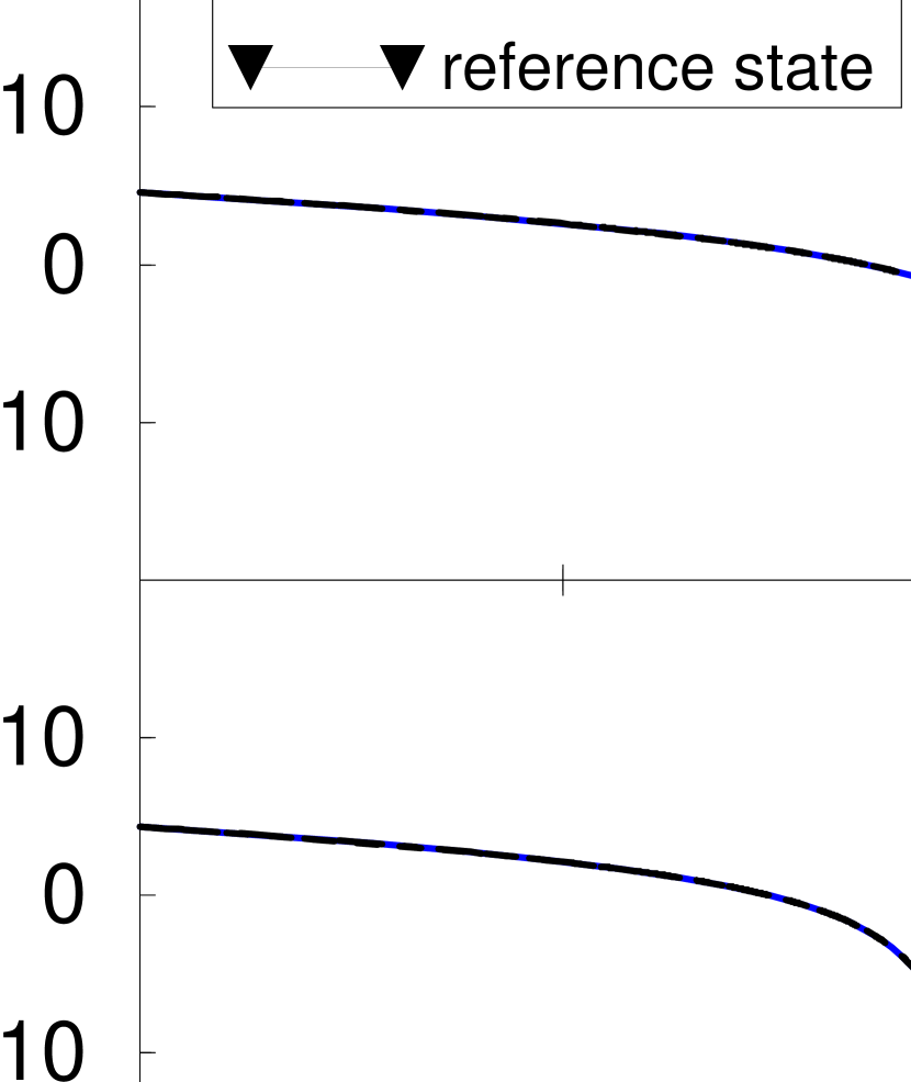
Figure 2: Transferability tests of the aluminum potential shown in Figure 1. Left panel: Logarithmic derivatives for the semilocal (dashed lines) and fully separable pseudopotentials (dot-dashed) vs. their all-electron counterparts (solid), as output by pswatch. Right panel: Error of the atomic excitation energies (open symbols) and the level spacing $\epsilon_{3s}-\epsilon_{3p}$ (filled symbols) calculated for the pseudo atom and the frozen-core all-electron atom.

Test of excitation energies – Next we verify that the pseudopotential reproduces the all-electron results for the atomic excitation or ionization energies, given by

$$E^{\rm M}_{ba}=E^{\rm tot-M}(\{f_{i}^{b}\})-E^{\rm tot-M}(\{f_{i}^{a}\})\quad\mbox{with M:}\left\{\begin{array}[]{l}\mbox{pseudopotential calculation (PS),}\\ \mbox{all-electron calculation (AE),}\\ \mbox{all-electron frozen-core calc. (FC),}\end{array}\right.$$ (29)

where $\{f_{i}^{b,a}\}$ denote the orbital occupancies in the excited and in the ground state configuration, respectively. The various expressions for $E^{\rm tot-M}$ are collected in the Appendix. This test seeks to emulate the cost in total energy associated with the orbital hybridization in different environments (“promotion energies”). The errors due to the use of pseudopotentials, $\Delta E^{\rm PS}_{ba}=E^{\rm PS}_{ba}-E^{\rm AE}_{ba}$ should be compared to $\Delta E^{\rm FC}_{ba}=E^{\rm FC}_{ba}-E^{\rm AE}_{ba}$, the errors that result from an all-electron calculation within the frozen-core approximation. There one recalculates just the valence states (with the full nodal structure), but keeps the core density fixed as in the ground state configuration $\{f_{i}^{a}\}$. Due to the variational principle, frozen-core calculations yield higher total energy values than unrestricted all-electron calculations where the core is allowed to relax, $E^{\rm tot-FC}(\{f^{b}_{i}\})\geq E^{\rm tot-AE}(\{f^{b}_{i}\})$, the equality holding only for $\{f_{i}^{a}\}$. In this test a transferable pseudopotential should perform with the same accuracy as the frozen-core all-electron calculation, $|\Delta E^{\rm PS}_{ba}|\simeq|\Delta E^{\rm FC}_{ba}|$, where the errors are typically of opposite sign for linearized core-valence exchange-correlation, and essentially the same if nonlinear core-valence exchange-correlation is taken into account. Typically, say for the first ionization potential, the errors do not exceed a few ten meV. Figure 2 shows the excitation energy error for an aluminum pseudopotential.

Test of level changes (chemical hardness) – As a last point we verify that the orbital eigenvalues for the pseudo atom closely track those of the all-electron atom when the orbital configuration changes. This test provides a discrete sampling of the atomic hardness matrix, $H_{ij}^{b}:=\frac{\partial}{\partial f_{i}}\epsilon_{j}(\{f_{k}^{b}\})=$ $\frac{\partial^{2}}{\partial f_{i}\partial f_{j}}E^{\rm tot}(\{f_{k}^{b}\})$ which ultimately governs the changes of the one-particle levels  [54, 55] and, by Janak’s theorem [63], of the total energy as functions of the orbital occupancies. Like for the excitation energies, the eigenvalues from the pseudopotential calculation are expected to agree with the all-electron results to within the error found for the frozen-core approximation, as seen in Fig. 2.

Convergence behavior

Figure 3: Convergence of the total energy in pseudopotential plane wave calculations of bulk GaAs, diamond, and fcc-Cu. Solid lines show the absolute total energy error (per electron) expected from the atomic pseudo wavefunctions using the estimate Eq. (32). Open circles show the actual values with respect to completely converged calculations. The weights $\{w_{l=0},w_{l=1},w_{l=2}\}$ taken in Eq. (32) were $\{2,1,0\}$ (Ga $4s^{2}4p^{1}4d^{0}$), $\{2,3,0\}$ (As $4s^{2}4p^{3}4d^{0}$), $\{2,2,0\}$ (C $2s^{2}2p^{2}3d^{0}$), and $\{1,0,10\}$ (Cu $3d^{10}4s^{1}4p^{0}$). Troullier-Martins pseudopotentials were employed with core cutoff radii $\{r^{c}_{l=0},r^{c}_{l=1},r^{c}_{l=2}\}$ (in bohr) of $\{2.2,2.3,2.5\}$ (Ga), $\{2.1,2.2,2.4\}$ (As), $\{1.5,1.5,1.5\}$ (C), and $\{2.1,2.3,2.1\}$ (Cu).

Checking the convergence behavior of the pseudopotentials with respect to the basis size is a basic task in calculating realistic systems, where the goal is to achieve convergence in total energy differences, e.g. binding energies, rather than the total energy itself. To provide some guidance in picking the smoothest out of a set of some similarly transferable pseudopotentials, and in choosing an initial estimate for a plane wave basis, the program pswatch evaluates the momentum space convergence of the atomic pseudo wavefunctions’ kinetic energy. This provides a measure for the (absolute) total energy convergence in applications [56]. Using the Fourier decomposition of the pseudo wavefunctions,

$$u^{\rm ps}_{l}(k)=\sqrt{\frac{2}{\pi}}\int_{0}^{\infty}krj_{l}(kr)u^{\rm ps}_{l}(r)\,dr\quad,$$ (30)

consider the error of the momentum space value of the kinetic energy as a function of the plane wave cutoff energy $E^{\rm pw}$ corresponding to the cutoff momentum $k^{\rm pw}=\sqrt{2E^{\rm pw}}$,

$$\Delta E^{\rm kin}_{l}(k^{\rm pw})=\int_{0}^{k^{\rm pw}}\frac{k^{2}}{2}\,|u^{\rm ps}_{l}(k)|^{2}dk-\int_{0}^{\infty}u^{\rm ps}_{l}(r)\left[-\frac{1}{2}\frac{d^{2}}{dr^{2}}+\frac{l(l+1)}{2r^{2}}\right]u^{\rm ps}_{l}(r)dr\quad.$$ (31)

The program pswatch computes the cutoff energies to achieve $\Delta E^{\rm kin}_{l}\leq 100,10,1\,\mbox{meV}$. For real systems a converged calculation typically corresponds to a plane wave cutoff that meets the criterion $\Delta E^{\rm kin}_{l}(k^{\rm pw})\leq 100\,\,\mbox{meV}$ for the pseudo atom [64]. A corresponding estimate of the (absolute) convergence of the total energy in poly-atomic systems is then given by the average of the errors $\Delta E^{\rm kin}_{l}$ over all states and atoms,

$$E^{\rm tot}(k^{\rm pw})-E^{\rm tot}(\infty)\simeq\sum_{l}w_{l}\Delta E^{\rm kin}_{l}(k^{\rm pw})\Bigl{|}_{{\rm atom}\,1}+\ldots\Bigl{|}_{{\rm atom}\,2}+\ldots\quad,$$ (32)

with the orbital weights $w_{l}$. Figure 3 illustrates this estimate.

2.5 Usage of pseudopotentials: Separation of long-ranged local and short-ranged nonlocal components

Operating with the ionic pseudopotential on the wavefunctions in a poly-atomic system requires their projection onto an angular momentum expansion, the second term of Eq. (2), which causes the predominant computational effort in calculating larger systems. As all components $V^{\rm ps}_{l}(r)$ at large $r$ reduce to the ionic Coulomb potential, $-Z^{\rm ion}/r$, getting independent of $l$. It is thus expedient to express the pseudopotential as a multiplicative local potential plus only a few $l$-dependent, short-ranged “corrections” for $l<l_{\rm max}$,

$$\!\!\!\langle{\bf r}|\hat{V}^{\rm ps}|{\bf r}^{\prime}\rangle = \langle{\bf r}|\hat{V}^{\rm loc}+\delta\hat{V}^{\rm sl}|{\bf r}^{\prime}\rangle$$ (33)

$$\rightarrow V^{\rm ps}_{l_{\rm loc}}(r)\delta({\bf r}-{\bf r}^{\prime})+\sum_{l=0}^{l_{\rm max}}\!\sum_{m=-l}^{l}\!Y^{\ast}_{lm}(\Omega_{{\bf r}})\delta V^{\rm sl}_{l}(r)\frac{\delta(r-r^{\prime})}{r^{2}}Y_{lm}(\Omega_{{\bf r}^{\prime}}),$$ (34)

where the local potential is taken as one of the semilocal pseudopotential components, $V^{\rm loc}(r)=V^{\rm ps}_{l=l_{\rm loc}}(r)$, and $\delta V^{\rm sl}_{l}(r)=V^{\rm ps}_{l}(r)-V^{\rm ps}_{l_{\rm loc}}(r)$ vanishes beyond $r^{\rm c}_{l}$. Typically one truncates the expansion at $l_{\rm max}=2$, whereby the core effects on the valence states with the same symmetries as the core states are accounted for. The number of projections is reduced most if one picks the $l_{\rm loc}=l_{\rm max}$ component as local potential $V^{\rm loc}(r)=V^{\rm ps}_{l_{\rm loc}}(r)=V^{\rm ps}_{l_{\rm lmax}}(r)$. Most preferably $l_{\rm loc}=l_{\rm max}=2$, the common practice for $sp$-type materials like silicon. We note that the local component of the pseudopotential in principle has to reproduce the scattering properties in the higher angular momentum channels with $l>l_{\rm max}$. Further aspects on the choice of the local potential come into play when one uses the fully separable form of the pseudopotential as discussed in the next Section.

2.6 Fully separable pseudopotentials and ghost states

Actual electronic structure codes mostly use the ionic pseudopotential in the fully separable form of Kleinman and Bylander (KB) [36]

$$\langle{\bf r}|\hat{V}^{\rm ps}|{\bf r}^{\prime}\rangle\quad = \quad\langle{\bf r}|\hat{V}^{\rm loc}+\delta\hat{V}^{\rm KB}|{\bf r}^{\prime}\rangle$$ (35)

$$\rightarrow \quad V^{\rm ps}_{l_{\rm loc}}(r)\delta({\bf r}-{\bf r}^{\prime})+\sum_{l=0}^{l_{\rm max}}\sum_{m=-l}^{l}\langle{\bf r}|\chi^{\rm KB}_{lm}\rangle E^{\rm KB}_{l}\langle\chi^{\rm KB}_{lm}|{\bf r}^{\prime}\rangle\quad,$$ (36)

where the short-ranged second term is a fully nonlocal rather than a semilocal operator in ${\bf r}$-space. Starting from a semilocal pseudopotential, the corresponding KB-pseudopotential is constructed such that it yields exactly the same pseudo wavefunctions and energies. This is accomplished with the projector functions

$$\langle{\bf r}|\chi^{\rm KB}_{lm}\rangle=\frac{1}{r}\chi_{l}(r)Y_{lm}(\Omega_{{\bf r}})=\frac{1}{r}\frac{u^{\rm ps}_{l}(r)\delta V^{\rm sl}_{l}(r)}{||u^{\rm ps}_{l}\delta V^{\rm sl}_{l}||^{1/2}}\,Y_{lm}(\Omega_{{\bf r}})\quad,$$ (37)

and the KB-energies

$$E^{\rm KB}_{l}=\frac{||u^{\rm ps}_{l}\delta V^{\rm sl}_{l}||}{\langle\psi^{\rm ps}_{lm}|\chi^{\rm KB}_{lm}\rangle}\quad,$$ (38)

with $||u^{\rm ps}_{l}\delta V^{\rm sl}_{l}||=\int_{0}^{\infty}u^{\rm ps}_{l}(r)\delta V^{\rm sl}_{l}(r)^{2}u^{\rm ps}_{l}(r)dr$  [65]. The KB-energy measures the strength of a nonlocal component relative to the local part of the pseudopotential, where the sign is determined by the KB-cosine $-1<\langle\psi^{\rm ps}_{lm}|\chi^{\rm KB}_{lm}\rangle<1$. Note that $\chi_{l}(r)\rightarrow 0$ as $\delta V^{\rm sl}_{l}(r)\rightarrow 0$ outside the core region. In poly-atomic systems the KB-form drastically reduces the effort of operating with the pseudopotentials on the wavefunctions, which causes the dominant computational workload in particular for larger systems: for an $N$-dimensional basis $\{|G_{i}\rangle\}$, the semilocal form requires the evaluation and storage of $\sim(N^{2}+N)/2$ matrix elements $\langle G_{i}|\delta\hat{V}^{\rm sl}_{l}|G_{j}\rangle$, with the KB-form these factorize, requiring just $\sim N$ projections $\langle G_{i}|\chi^{\rm KB}_{lm}\rangle$ and simple multiplications $\langle G_{i}|\chi^{\rm KB}_{lm}\rangle E^{\rm KB}_{l}\langle\chi^{\rm KB}_{lm}|G_{j}\rangle$.

In transforming a semilocal to the corresponding KB-pseudopotential one needs to make sure that the KB-form does not lead to unphysical “ghost” states at energies below or near those of the physical valence states as these would undermine its transferability. Such spurious states can occur for specific (unfavorable) choices of the underlying semilocal and local pseudopotentials. They are an artifact of the KB-form’s nonlocality by which the nodeless (reference) pseudo wavefunctions need not be the lowest possible eigenstate, unlike for the semilocal form [37]. Formally the KB-form can be generalized to a series expansion of a fully nonlocal pseudopotential which avoids ghost states by projecting onto additional reference states in Eq. (36)  [66], yet at the cost of somewhat increasing the computational labor. In practice transferable ghost-free KB-pseudopotentials are readily obtained by a proper choice of the local component ($l_{\rm loc}$) and the core cutoff radii ($r^{\rm c}_{l}$) in the basic semilocal pseudopotentials. In the next paragraphs we discuss how to identify and remove ghost states using the utility pswatch.

First of all a ghost state is indicated by a marked deviation of the logarithmic derivatives of the KB-pseudopotential from those of the respective semilocal pseudopotential or all-electron potential. Note that such features can be delicate to detect if the energy sampling is too coarse to resolve them or if they occur below the inspected energy interval. The program pswatch provides the logarithmic derivatives on an adaptive energy mesh, integrating the nonlocal radial Schrödinger equation for the KB-pseudopotential,

$$\left[-\frac{1}{2}\frac{d^{2}}{dr^{2}}+\frac{l(l+1)}{2r^{2}}+V^{\rm ps,scr}_{l_{\rm loc}}(r)-\epsilon\right]u^{\rm ps}_{l}(\epsilon;r)+\chi_{l}(r)E_{l}\int_{0}^{\infty}\!\chi_{l}(r^{\prime})u^{\rm ps}_{l}(\epsilon;r^{\prime})\,dr^{\prime}=0\quad,$$ (39)

with $E_{l}\equiv E^{\rm KB}_{l}$, from the origin up to a diagnostic radius, as described in Ref. [37].

Secondly, ghost states are revealed in a comparison of the atomic bound state spectra for the semilocal and the KB-pseudopotentials [67], i.e., as extra levels not present in the true valence spectrum. The program pswatch solves the respective eigenvalue problem, Eq. (39), using Laguerre polynomials as a numerically convenient basis [68].

Thirdly, ghost states below the valence states are identified by a rigorous criterion by Gonze et al. [37]. The program pswatch evaluates this criterion, here we summarize its key points. For a given angular momentum, consider the spectrum $\{\tilde{\epsilon}_{i}(E_{l})\}$ of the nonlocal Hamiltonian associated with the KB-form, Eq. (39), as a function of the strength parameter $E_{l}$. Comparing to the spectrum resulting from the local part of the (screened) pseudopotential alone, $\{\tilde{\epsilon}_{i}(E_{l}\equiv 0)\}$, the eigenvalues always satisfy the sequences [37],

$$\tilde{\epsilon}_{0}(0)<\tilde{\epsilon}_{0}(E_{l})<\tilde{\epsilon}_{1}(0)<\tilde{\epsilon}_{1}(E_{l})<... \quad\mbox{if}\quad E_{l}>0\quad,$$ (40)

$$\tilde{\epsilon}_{0}(E_{l})<\tilde{\epsilon}_{0}(0)<\tilde{\epsilon}_{1}(E_{l})<\tilde{\epsilon}_{1}(0)<... \quad\mbox{if}\quad E_{l}<0\quad.$$ (41)

Now the actual KB-pseudopotential gives $E_{l}\equiv E^{\rm KB}_{l}$. The reference eigenvalue $\epsilon^{\rm ps}_{l}$ which it reproduces by construction corresponds to one of the levels $\{\tilde{\epsilon}_{0,1,\ldots}(E_{l}=E^{\rm KB}_{l})\}$. If it corresponds to the ground state level, i.e. $\epsilon^{\rm ps}_{l}\equiv\tilde{\epsilon}_{0}(E_{l}=E^{\rm KB}_{l})$, obviously no lower (ghost) state exists. Whether this holds true is decided from (40) or (41) with the help of the eigenvalues for the local potential: There is no ghost level beneath the reference level $\epsilon^{\rm ps}_{l}$ for

$$E^{\rm KB}_{l}>0 \tilde{\epsilon}_{0}(0)<\epsilon^{\rm ps}_{l}<\tilde{\epsilon}_{1}(0)$$ if the reference level lies below the first excited level of the local potential, in Eq. (40), (42)

$$E^{\rm KB}_{l}<0 \epsilon^{\rm ps}_{l}<\tilde{\epsilon}_{0}(0)$$ if the reference level lies below the ground state level of the local potential, Eq. (41). (43)

The program pswatch reports ghost states based on this criterion.

As a practical rule ghost-free KB-pseudopotentials may be obtained with the $d$-component as the local potential except for “two-shell” situations like the transition metal elements where typically the $s$-component is used as the local potential. To eliminate a ghost state occurring for some $l$ one may (i) change $l_{\rm loc}$, i.e. use a different component of the semilocal pseudopotential as the local potential, (ii) adjust the core cutoff radii $r^{c}_{l}$ of the offending component $V^{\rm ps}_{l}(r)$ or the local potential $V^{\rm ps}_{l_{\rm loc}}(r)$, respectively. In doing so the basic transferability ought to be maintained (see Sec. 2.4). Also, it is expedient to take $l_{\rm loc}=l_{\rm max}$ in order to keep the number of the (computationally intensive) projections implied by Eq. (36) small. Modifying the above entities seeks to adjust $E^{\rm KB}_{l}$, i.e. the strength of the KB-pseudopotential relative to the local potential such that either (42) or (43) is satisfied. Note that a repulsive enough local potential (achieved e.g. by increasing $r^{c}_{l_{\rm loc}}$ or taking $l_{\rm loc}=0$) rules out any ghost state: Such a potential eventually leads to a negative KB-energy (38) as $\delta V^{\rm sl}_{l}(r)=V^{\rm ps}_{l}(r)-V^{\rm loc}(r)<0$. Also, $\tilde{\epsilon}_{0}(0)\rightarrow 0$ since such a local potential gives at most a weakly bound ground state. As $E^{\rm KB}_{l}<0$ one has $\epsilon^{\rm ps}_{l}<\tilde{\epsilon}_{0}(0)\approx 0$ by virtue of (41), ruling out any ghost level.

Table 1: Analysis of ghost states for the Kleinman-Bylander pseudopotential of Cu employing Eq. (42) and (43). The eigenvalus for the local potential are underlined. The semilocal pseudopotentials were constructed for the $(3d^{10}\,4s^{2}\,4p^{0})$-configuration, using the Troullier-Martins scheme with cutoff radii $r^{c}_{4s}=r^{3d}_{l=2}\simeq 2.1$ bohr and $r^{c}_{4p}\simeq 2.3$ bohr. Exchange-correlation was treated within the LDA.

$l_{\rm loc}$	$l$	$E^{\rm KB}_{l}$ (eV)	bound state energies (eV)				ghost?
$2\,(3d)$	$0\,(4s)$	319.67	$-219.06$	$-72.98$	$-15.95$	$-4.86$	yes
			$\tilde{\epsilon}_{0}(0)$	$\tilde{\epsilon}_{0}(E^{\rm KB}_{l})$	$\tilde{\epsilon}_{1}(0)$	$\tilde{\epsilon}_{1}(E^{\rm KB}_{l})\equiv\epsilon^{\rm ps}_{4s}$
	$1\,\,(4p)$	223.44	$-108.75$	$-0.77$		$-0.46$	no
			$\tilde{\epsilon}_{0}(0)$	$\tilde{\epsilon}_{0}(E^{\rm KB}_{l})\equiv\epsilon^{\rm ps}_{4p}$		$\tilde{\epsilon}_{1}(0)$
$0\,(4s)$	$2\,(3d)$	$-273.80$	$-5.33$				no
			$\tilde{\epsilon}_{0}(E^{\rm KB}_{l})\equiv\epsilon^{\rm ps}_{3d}$
	$1\,\,(4p)$	51.64	$-0.92$	$-0.77$			no
			$\tilde{\epsilon}_{0}(0)$	$\tilde{\epsilon}_{0}(E^{\rm KB}_{l})\equiv\epsilon^{\rm ps}_{4p}$

Table 1 illustrates the foregoing for a copper pseudopotential (see also Ref. [37] and the examples in this package’s distribution): the $3,4,5d$-component taken as local potential ($V^{\rm loc}=V^{\rm ps}_{l_{\rm max}}$) acts as a strongly attractive potential on the $s$-states. Accordingly the eigenvalue sequence starts at quite low an energy. In the case of copper the reference energy of the $4s$-pseudopotential lies already above the first excited level for the local potential, $\tilde{\epsilon}_{1}(0)<\epsilon_{4s}$. By Eqs. (41) or (40) the Cu $4s$-level corresponds to an excited $s$-like level of the KB-pseudopotential, and so there is a ghost state beneath the Cu $4s$-state. By contrast, taking the $s$-component as the local potential results in a ghost-free KB-pseudopotential.

3 Description of the package

The package fhi98PP provides as main utilities the UNIX C-shell scripts psgen and pswatch. The script psgen and the related FORTRAN program fhipp solve the all-electron atom and generate the ionic pseudopotentials (see Secs.  2.1 – 2.3). The script pswatch and the related FORTRAN program pslp solve the pseudo-atom for a given pseudopotential, and carry out tests to monitor the pseudopotential’s transferability in its semilocal and fully separable form (see Secs.  2.4 – 2.6). The shell scripts serve as command line interfaces for running the FORTRAN programs. For visual inspection of results, they group output into thematic graphic files to be viewed with the public domain, X-Windows based plotting tools XVGR or XMGR [69]. The scripts include command summaries (execute psgen -h or pswatch -h). The Tables 2 – 4 explain the required and the optional input of psgen and pswatch. The Tables 5 – 7 summarize the meaning of the input and output files, and display their dependencies on the FORTRAN routines. All input and output files reside in the chosen working directory. The name of the input files can be chosen freely. For the output files, the shell scripts compose filenames from a freely chosen mnemonic identifier and preset functional suffixes. For example, “al.cpi” shall denote an output file which tabulates an aluminum pseudopotential.

The supplement “Test run protocol” at the end of this paper provides a prototype session protocol for generating pseudopotentials, for aluminum as an example. A database of input files is distributed along with the package (see Sec. 3.3). Below we outline the structure of the shell scripts and the related FORTRAN programs, and then discuss the various input variables.

3.1 The tool psgen for solving the all-electron atom and generating pseudopotentials

The script psgen reads from the commandline the identifier string name, and prinicpal input file $<$input data$>$ containing the atomic configuration and run parameters as explained below.

psgen -o name $<$input data$>$, the standard mode, performs the all-electron calculation and constructs the pseudopotentials. Chief output is the run protocol name.dat and the pseudopotential data file name.cpi.

psgen -o name -fc name.fc $<$input data$>$, the frozen-core mode, performs the all-electron calculation within the frozen-core approximation. There only the valence orbitals are determined self-consistently while the core density is held fixed as given by the file name.fc (see below). This is meant to generate a certain pseudopotential component from an excited configuration with the unrelaxed core density of the ground state, and also to establish benchmark values, e.g. for excitation energies, in transferability tests.

psgen -ao -o name $<$input data$>$, the atom-only mode, carries out just the all-electron calculation, as needed for instance to determine excitation energies.

The option -e invokes an editor for the input file $<$input data$>$ The command psgen -h lists all command options.

The prinicpal input file ($<$input data$>$, e.g. called al.ini) specifies the electronic configuration of the atom, the partitioning of core and valence states, as well as parameters for handling exchange-correlation and constructing the pseudopotentials. Below we discuss the main variables, the Tables 2 and 3 give an overview. Table 4 describes a sample file.

The variable $z$ stands for the atomic number. Non-integer values to realize artificial atoms are allowed.

The variables $nc$ and $nv$ specify the number of core states and the number of valence states, respectively. Note that the norm-conservation constraints can be met exactly for one and only one valence state per angular momentum channel (see Sec. 2.2).

The variable $iexc$ specifies the exchange-correlation scheme used in solving the all-electron atom and in the unscreening of the pseudopotentials. Table 4 lists the implemented parameterizations of the local-density approximation and the generalized-gradient approximations (see Sec. 2.1). On the commandline $iexc$ is set by psgen -xc $iexc$ … .

The variable $rnlc$ controls the handling of core-valence exchange-correlation in the unscreening of the pseudopotential and the construction of a partial core density (see Sec. 2.3). Setting $rnlc=0$ corresponds to the ordinary linear treatment, a partial core density is not computed. Taking $rnlc>0$ implies the explicit treatment of core-valence XC with the help of a partial core density. The value of $rnlc$ specifies the cutoff radius (in bohr) beyond which the partial core density is identical with the actual true core electron density. The respective command is psgen -rc 1.3 …, e.g., setting $rnlc=1.3$ bohr. The partial core density is appended to the file name.cpi. If the all-electron calculation is done in the frozen-core mode, the partial core density is constructed from the input core electron density.

The variables $n(i)$, $l(i)$, and $f(i)$ denote the $i$-th state’s principal quantum number, angular momentum quantum number, and occupation number, respectively. The $i=1,...,nc$ core states need to be listed before the $i=nc+1,...,nc+nv$ valence states. The principal quantum numbers should appear in ascending order, $n(i)\geq n(i-1)$. Unoccupied valence states which are not listed are assumed to be “unbound”, the respective pseudopotential is then calculated by the Hamann procedure (see Sec. 2.2). Listing such states with $f(i)=0$ instructs the program to determine the respective state. Note that negatively charged ions, $\sum_{i=1}^{nc+nv}f(i)>z$, are unstable within LDA or GGA, and may cause the calculation to fail.

The variable $lmax$ specifies the highest angular momentum channel up to which the program constructs pseudopotential components. The variable $s\_pp\_def$ allows to select either the Hamann scheme $s\_pp\_def=\mbox{\sf h}$ or the Troullier-Martins scheme $s\_pp\_def=\mbox{\sf t}$ for constructing the pseudopotentials. Appropriate default cutoff radii are supplied by the program. psgen -T $s\_pp\_type$ … is the related script command.

Any further input is optional and serves to override the default settings in the angular momentum channel $lt$ for the cutoff radius $rct$ (in bohr), the reference energy $ect$ (in eV), and the pseudopotential scheme $s\_pp\_type$. This feature is mainly for finetuning the cutoff radii when a ghost state of the Kleinman-Bylander form has to be eliminated (see Sec. 2.6). If the cutoff radii are enlarged in order to achieve softer pseudopotentials, the transferability of the resulting pseudopotential should be carefully verified. On the commandline, the options -rs, -rp, -rd, -rf may be used to set the cutoff radii of the $s,p,d,f$-components of the pseudopotentials. For instance psgen -rp 1.5 … sets the $p$-cutoff radius to $1.5$ bohr.

By the commandline option -r one instructs psgen to perform a non-relativistic all-electron calculation rather than a scalar-relativistic one (default). The corresponding variable $tnrl$ is then set to true.

By the commandline option -g all FORTRAN input and output files are saved, rather than being removed upon exiting psgen.

The script psgen first generates appropriate input files (fort.20 and fort.22) used by the FORTRAN routine fhipp which it invokes next. If the frozen-core mode is applied, the core density name.fc is copied to fort.18 (see also below). After completion of fhipp the script writes a descriptive protocol to the file name.dat. It then generates the file name.cpi which contains the components of the ionic pseudotential, the pseudo wavefunctions, and, optionally, any partial core density on a logarithmic radial grid, adapted to the format used in the fhi96md electronic-structure and molecular-dynamics package [9]. If different reference configurations are used in constructing the pseudopotential components, a customized file name.cpi can be created from the corresponding FORTRAN output files fort.40, etc., described in Table 7. The output file name.aep contains the all-electron full potentials, and will be used by the utility pswatch to evaluate the all-electron logarithmic derivatives. The file name.fc lists the full core electron density, and may be used as input to psgen in a subsequent frozen-core calculation. Moreover the script produces various graphical files for visual inspection of, e.g., the ionic pseudopotential (file xv.name.pspot_i) or the all-electron wavefunctions (file xv.name.ae_wfct).

In the pertinent FORTRAN program fhipp the main routine fhipp initially reads the run attributes and atomic configuration from the unformatted files fort.20 and fort.22. A logarithmic radial mesh is set up, $\{r_{m}=a^{m-1}_{\rm mesh}r_{\rm min}(Z)\quad|\quad m=1,2,...,m_{\rm max}\}$, with default parameters as set in the FORTRAN header file default.h. All numerical integrations are done on this mesh. Any core electron density is read in from fort.18, and must be tabulated on the current radial mesh. The subroutine sratom_n self-consistently solves for the all-electron atomic eigenstates and the full potential. The radial Schrödinger equations are integrated by a predictor-corrector scheme in the subroutine dftseq. The self-consistency cycle stops once all eigenvalues are converged. The program then writes a run protocol to fort.23, the all-electron wavefunctions to fort.38, the full core density to fort.19, and the full all-electron potential to fort.37. If the atom-only mode is applied, the program exits at this point. Otherwise the main routine next determines the default parameters for constructing the pseudopotentials, and checks for any optional input in fort.22 to override the default settings. The subroutine ncpp then determines the pseudo wavefunctions and the screened pseudopotentials. The program proceeds with the unscreening of the pseudopotentials. Optionally the subroutine dnlcc constructs an appropriate partial core density, either from the self-consistent full core density or from the user provided frozen-core density. Finally a protocol of the pseudopotential construction is appended to fort.23. The ionic pseudopotential and the pseudo wavefunction of each angular momentum channel $l$ are written to fort.4[$l=0,1,...$]. The components of the screened pseudopotential are written to fort.45 ($l=0$), fort.46 ($l=1$), etc. . The partial core density is output to fort.27. All quantities are tabulated on the dense logarithmic mesh that was employed in computing them, except for the all-electron wavefunctions which are output on a sparser mesh.

3.2 The tool pswatch for solving the pseudo atom and checking pseudopotentials

The script pswatch is normally run after psgen. It reads from the command line the identifying string name, and the name of the principal input file $<$input data$>$ for the atomic valence configuration. The latter has the same layout as when generating the pseudopotentials (see Sec. 3.1). Furthermore pswatch assumes the presence of the files name.cpi (ionic pseudopotentials) and name.aep (all-electron potential). Both are routinely provided by a run of psgen as described above. The same radial grid must be used in these files. Also, the all-electron potential should be consistent with the present atomic configuration. Several run modes are implemented:

pswatch -i name $<$input data$>$, the standard mode, performs first a self-consistent calculation of the pseudo-atom, then computes the logarithmic derivatives for the all-electron potential and the screened pseudopotential, and carries out the ghost state analysis for the fully separable pseudopotential.

pswatch -ao -i name $<$input data$>$, the atom-only mode, just solves the pseudo-atom, e.g., in order to determine excitation energies.

pswatch -kb -i name $<$input data$>$, the semilocal-only mode, skips the ghost state analysis.

The option -e invokes an editor for the input file $<$input data$>$. The command pswatch -h gives a list of all options.

Several parameters that control the evaluation of the logarithmic derivatives and the handling of the fully separable pseudopotential can be specified on the command line. The script pswatch collects them in an auxiliary input file (fort.21). Below we introduce the main parameters, the Tables 2 and 3 list them in full. Sample input files are given in Table 4.

The variable $lmax$ specifies the angular momentum channel up to which pseudopotential components are present. For $l\leq lmax$ the program uses the respective components to compute the logarithmic derivatives. For $l>lmax$ it uses the local potential instead.

The variable $lloc$ denotes the angular momentum channel whose pseudopotential component should be taken as the local potential, with $lloc\leq lmax$. For instance the $s$-component is chosen by the pswatch -l 0 … command.

The variable $rlgd$ gives the diagnostic radius (in bohr) at which the logarithmic derivatives are evaluated. If $rlgd=0$ the program assigns as a default value the covalent radius for the atom at hand. Note that the diagnostic radius should be larger than the cutoff radii used in constructing the pseudopotential. The according command is, e.g., pswatch -rl 2.5 …, setting $rlgd=2.5$ bohr.

The commandline option pswatch -cpo $<$outfile$>$ … causes the program to use for the analysis of the Kleinman-Bylander form the self-consistently calculated pseudo wavefunctions rather than those provided by the file name.cpi (default). The calculated wavefunctions will be written to a file outfile analogous to name.cpi. This feature may be used, e.g., when just the ionic pseudopotential but not the respective pseudo wavefunctions are known. The corresponding variable tiwf true is then set true.

The commandline option -r instructs pswatch to calculate the logarithmic derivatives for the all-electron potential non-relativistically rather than scalar-relativistically (default). The corresponding variable $tnrl$ is then set true.

By the commandline option -g all FORTRAN input and output files are saved, rather than being removed upon exiting psgen.

The script sets up appropriate input for the FORTRAN program pslp which is invoked next. A self-evident protocol is printed to the terminal and also written to the file name.test. Upon completion, pswatch assembles the file xv.name.lder for the visual inspection of the logarithmic derivatives of the all-electron potential and pseudopotentials.

In the FORTRAN program pslp the main routine pslp reads the run attributes and atomic valence configuration from the unformatted files fort.21 and fort.22, the latter having the same layout as for the fhipp program. Next it reads from fort.31 the (logarithmic) radial mesh, the pseudo wavefunctions to be used in the Kleinman-Bylander construction, the components of the ionic pseudopotential, and, if present, the partial core density. The program writes a run protocol to standard output. The subroutine psatom first self-consistently solves for the wavefunctions and the screening potential of the pseudo atom. The self-consistency cycle stops once all eigenvalues have converged. The program then writes the semilocal ionic pseudopotential and the computed pseudo wavefunctions to fort.4[$l=0,1,...$], the related screened pseudopotential to fort.45, fort.46, etc., and any partial core density to fort.27. If the atom-only mode is applied, the program stops at this point. Otherwise the subroutine ppcheck proceeds with the evaluation of logarithmic derivatives. This is done for a user-specified or a preset diagnostic radius. An adaptive energy mesh is employed, where the upper and lower bounds may be adjusted in the FORTRAN source file ppcheck.f. As the first step, the all-electron potential is read in from the file fort.37. It must be given on the same radial mesh as the pseudopotentials. Integrating the radial Schrödinger equation for each angular momentum channel $l$, the all-electron logarithmic derivative is output to fort.5[$l=0,1,...$]. The corresponding logarithmic derivative of the self-consistently screened semilocal pseudopotential is tabulated in fort.6[$l=0,1,...$]. Next, ppcheck transforms the pseudopotential into the fully separable form (see Sec. 2.6). By default the inputted pseudo wavefunctions (file name.cpi) are used to set up the projector functions, optionally they are substituted by the pseudo wavefunctions obtained earlier in psatom. The subroutine derlkb then evaluates the logarithmic derivative for the respective nonlocal radial Schrödinger equation, which is output to fort.7[$l=0,1,...$]. In the next step, klbyii computes the bound state spectra for the semilocal and nonlocal pseudopotentials. Furthermore ppcheck examines the fully separable potentials for ghost states. Finally the subroutine kinkon evaluates the kinetic energy for each calculated pseudo wavefunction in momentum space (see Sec. 2.4).

3.3 Set-up of the package

The package fhi98PP is distributed as a tar-archive which can be unpacked by the UNIX command tar. The directory Dfhipp forms the root of the package’s directory tree.

In the directory Dplay we supply sample input and output files for several exemplary pseudopotentials (aluminum, sodium, arsenic, selenium, and nitrogen), along with a detailed tutorial (as Postscript file). These examples should illustrate on a rather “hands-on” level the procedure for constructing pseudopotentials.

The directory bin/Tools contains the shell scripts to generate (psgen) and validate (pswatch) the pseudopotentials. Also provided are some self-explanatory shell scripts (psdata_al, pstrans) to assist with the transferability tests discussed in Sec. 2.4. In the directory bin/Elements we supply a database of inputfiles used in constructing the pseudopotentials. These have the generic names chemical_symbol:h.ini for the Hamann, and chemical_symbol:tm.ini for the Troullier-Martins scheme. The directory bin/Xvgr contains the header files for the graphics output produced by the shell scripts.

The directory src includes the sources and libraries of the program, as well as the Makefile for the compilation of the FORTRAN programs fhipp and pslp that are invoked by the shell scripts. Both programs use linear algebra routines which need to be linked either from the ESSL-library or from a subset of the public domain LAPACK-routines. The latter is included as a library (libFREE) in the directory lib, and may be compiled either as specified in the Makefile, or, alternatively, simply along with the other routines.

In order to run the package’s tools psgen or pswatch one has to create the executables fhipp.x and pslp.x. To this end one first needs to properly set in the Makefile the name of the FORTRAN compiler, the compiler and linker flags, and specify whether the ESSL or libFREE library should be invoked. Executing the UNIX command make all then does the compilation. Secondly, one needs to specify in the scripts psgen and pswatch the correct source paths for the FORTRAN executables and the graphics header files. We suggest to install the shell scripts psgen and pswatch as personalized commands. Note that for viewing the graphics output from psgen and pswatch one of the public domain packages XMGR or XVGR must be available as well.

4 Test run

In the test run one calculates a Hamann-type pseudopotential for aluminum. To this end one executes psgen al -o al:h as command. This will copy the inputfile al:h.ini from the database bin/Elements into the present working directory, run the program fhipp and process its outputfiles into the various text and graphics files as described above. Secondly, one evaluates the logarithmic derivatives and performs the ghost state analysis. This is done by executing the command pswatch -i al:h al:h.ini, which will produce output on the terminal as well as to various text and graphics files described in Sec. 3. Samples of the principal output and a terminal session protocol are listed in the Section “Test run protocol”. A full set of the input and output files of the test run is given in the directory sample. Further examples can be found in the directory Dplay.

Appendix

This appendix lists total energy expressions computed by the utilities psgen and pswatch.

All-electron atom – The total energy of the spherical atom for a given set of occupancies $f_{nl}$ (corresponding to a ground- or excited state) is obtained from the radial wavefunctions $u_{nl}(r)$ and electron density $\rho(r)=\frac{1}{4\pi r^{2}}\sum_{nl}f_{nl}|u_{nl}(r)|^{2}$ as layed out in Sec. 2.1,

$$E^{\rm tot-AE}[\rho]=T[\rho]+E^{\rm XC}[\rho]+E^{\rm H}[\rho]+\int-\frac{Z}{r}\rho(r)\,d^{3}r\quad,$$ (44)

with the Hartree energy $E^{\rm H}[\rho]=\frac{1}{2}\int V^{\rm H}[\rho;r]\rho(r)\,d^{3}r$ (10), the exchange-correlation energy $E^{\rm XC}$ in LDA (12) or GGA (14), and the kinetic energy

$$T[\rho]=\sum_{nl}f_{nl}\epsilon_{nl}-\int V[\rho;r]\rho(r)\,d^{3}r\quad,$$ (45)

stated in terms of the one-particle or orbital energy, $\sum_{nl}f_{nl}\epsilon_{nl}$, and the potential energy due to the effective potential $V[\rho;r]$ (9).

Frozen-core all-electron atom – When the atom is calculated in the frozen-core approximation only the valence states are determined self-consistently. The core density is taken over from a previously solved atomic reference state, in the following indicated by zero sub- and superscripts. The effective potential (9) is obtained with the electron density

$$\rho(r)=\rho^{\rm core}_{0}(r)+\rho^{\rm val}\quad\mbox{with}$$ (46)

$$\rho^{\rm core}_{0}(r)=\frac{1}{4\pi r^{2}}\sum_{nl}^{\rm core}f_{nl}\left|u_{nl}^{(0)}(r)\right|^{2}\quad,\quad\mbox{and}\quad\rho^{\rm val}(r)=\frac{1}{4\pi r^{2}}\sum_{nl}^{\rm val}f_{nl}\left|u_{nl}(r)\right|^{2}\quad,$$ (47)

and the kinetic energies of the core and valence electrons are given by

$$T^{\rm core}[\rho_{0}]=\sum_{nl}^{\rm core}f_{nl}\epsilon_{nl}^{(0)}-\int V[\rho_{0};r]\rho^{\rm core}_{0}(r)d^{3}r\quad,$$ (48)

$$T^{\rm val}[\rho]=\sum_{nl}^{\rm val}f_{nl}\epsilon_{nl}-\int V[\rho;r]\rho^{\rm val}(r)d^{3}r\quad.$$ (49)

The atomic total energy in the frozen-core approximation then reads

$$E^{\rm tot-FC}[\rho_{0};\rho]=T^{\rm core}[\rho_{0}]+T^{\rm val}[\rho]+E^{\rm XC}[\rho]+E^{\rm H}[\rho]+\int-\frac{Z}{r}\rho(r)d^{3}r\quad.$$ (50)

For the reference configuration, i.e. $\rho\equiv\rho_{0}$, the unconstrained and frozen-core total energies (44) and (50) take on the same value.

Pseudo atom – For a given set of valence occupancies $f_{l}$ the pseudo valence states are determined by self-consistently solving the radial Schrödinger equations associated with the semilocal pseudopotential,

$$\left[-\frac{1}{2}\frac{d^{2}}{dr^{2}}+\frac{l(l+1)}{2r^{2}}+V^{\rm HXC}(r)+V^{\rm ps}_{l}(r)-\epsilon^{\rm ps}_{l}\right]u^{\rm ps}_{l}(r)=0\quad,$$ (51)

with the screening potential

$$V^{\rm HXC}(r)=V^{\rm XC}[\rho^{\rm ps}+\tilde{\rho}^{\rm core}_{0};r]+V^{\rm H}[\rho^{\rm ps};r]\quad,$$ (52)

and $\rho^{\rm ps}(r)=\frac{1}{4\pi r^{2}}\sum_{l}f_{l}\left|u^{\rm ps}_{l}(r)\right|^{2}$. The total energy of the pseudo atom is given by

$$E^{\rm tot-PS}[\rho^{\rm ps}]=T[\rho^{\rm ps}]+E^{\rm XC}[\rho^{\rm ps}+\tilde{\rho}^{\rm core}_{0}]+E^{\rm H}[\rho^{\rm ps}]+\sum_{l}f_{l}\int_{0}^{\infty}V^{\rm ps}_{l}(r)|u^{\rm ps}_{l}(r)|^{2}\,dr\quad,$$ (53)

where the kinetic energy associated with the pseudo valence states is

$$T[\rho^{\rm ps}]=\sum_{l}f_{l}\left(\epsilon^{\rm ps}_{l}-\int_{0}^{\infty}\left\{V^{\rm HXC}(r)+V^{\rm ps}_{l}(r)\right\}|u^{\rm ps}_{l}(r)|^{2}\,dr\right)\quad.$$ (54)

For the nonlinear core-valence exchange-correlation scheme, $E^{\rm XC}$ and $V^{\rm XC}$ depend on the particular partial core density $\tilde{\rho}^{\rm core}_{0}(r)$ (see Sec. 2.3).

Table 2: Atomic configuration and pseudopotential parameters, given in the input file name.ini of the scripts psgen and pswatch (file fort.22 of the FORTRAN routines).

variable	type	values
required input, psgen and pswatch
$z$	real	$>\,0$	atomic number (nuclear charge)
$nc$	integer	$\geq\,0$	number of core states
$nv$	integer	$\geq\,0$	number of valence states
$rnlc$	real	$=\,0$	linearized core-valence exchange-correlation
		$>\,0$	nonlinear core-valence exchange-correlation,
			using a partial core inside the radius rnlc (in bohr)
$iexc$	integer		exchangex-correlationc approximation
		1	LDA Wignerc [49]
		2	LDA Hedin/Lundquistc [48]
		3	LDA Perdew/Zungerc ’81 [47]
		4	GGA Perdew/Wangxc ’91 [27]
		5	GGA Beckex, Perdewc ’86 [30, 31]
		6	GGA Perdew/Burke/Ernzerhofxc [28]
		7	LDA Perdew/Wangc ’92 [29] $+$ relativistic
			correctionx of MacDonald/Vosko [59]
		8	LDA Perdew/Wangc ’92 [29]
		9	GGA Beckex, Lee/Yang/Parrc [30, 32]
		10	GGA Perdew/Wangx ’91, Lee/Yang/Parrc [27, 32]
$n(i)$	integer		principal quantum number of state $i$ states should be in ascending order w.r.t. to $n(i)$
$l(i)$	integer		angular momentum quantum number of state $i$
$f(i)$	real		occupancy number of level $i$
required input, psgen only
$lmax$	integer	0 … 4	maximum $l=l_{\rm max}$ to generate pseudopotential for
$s\_pp\_def$	character	h	Hamann pseudopotential scheme
		t	Troullier/Martins pseudopotential scheme
optional input, psgen only
$lt$	integer	0 … 4	for $lt$-th pseudopotential component:   use alternate cutoff radius and/or reference energy and/or scheme from present line
$rct$	real	$=\,0$	core cutoff radius, use default
		$>\,0$	use this value (in bohr) instead
$et$	real	$=\,0$	reference energy, use default:    for an occupied state its eigenvalue, for an unoccupied state the highest eigenvalue of the occupied states
		$\neq\,0$	use this value (in eV) instead
$s\_pp\_type$	character	-	pseudopotential scheme, use $s\_pp\_def$
		h, t	see required input

Table 3: Upper section: Control parameters for the FORTRAN routine fhipp invoked by the script psgen, and passed by the input file fort.20. Lower section: The same for the FORTRAN routine pslp invoked by the script pswatch, and passed by the input file fort.21. These files are created by and depend on the arguments given to the shell scripts.

variable	type	values
file fort.20 of fhipp (optional input)
tdopsp	logical	true	compute pseudopotential (default)
		false	atom-only mode:   stop after solving all-electron atom
tnrl	logical	true	non-relativistic all-electron atom
		false	dto. scalar-relativistic (default)
file fort.21 of pslp (required input)
lloc	integer	$0\ldots l_{\rm max}$	use $lloc$-th pseudopotential component as the local potential
lbeg	integer	$0\ldots l_{\rm max}$	lowest angular momentum channel to calculate logarithmic derivatives for
lend	integer	$0\ldots l_{\rm max}$	highest angular momentum channel to calculate logarithmic derivatives for
lmax	integer	$l_{\rm max}\geq 0$	angular momentum number up to which pseudopotential components are present for, apply the local potential in any higher channel
rlgd	real	$\geq\,0$	diagnostic radius where the logarithmic derivatives are computed, ought be outside the core region
tlgd	logical	true	evaluate logarithmic derivatives (default)
		false	dto. skipped
tkb	logical	true	analyze Kleinman-Bylander potentials (default)
		false	dto. skipped
tiwf	logical	true	use input pseudo wavefunctions for the construction of Kleinman-Bylander potentials (default)
		false	dto. but use calculated waves
tnrl	logical	true	assume non-relativistic all-electron calculation in the calculation of the logarithmic derivatives
		false	dto. scalar-relativistic (default)

Table 4: Sample input files to construct and validate an aluminum pseudopotential.

Atomic configuration and pseudopotential parameters (file al.ini of shell scripts, file fort.22 of FORTRAN routines)

13.00 3 2 8 0.0 1 0 2.00 2 0 2.00 2 1 6.00 3 0 2.00 3 1 1.00 2 h 0 1.25 0.00 h 1 1.40 0.00 h z nc nv iexc rnlc n(i) l(i) f(i) . . . . lmax s_pp_def lt rct et s_pp_type .

control parameters of fhipp (file fort.20 created by psgen)

.t. .t. tdopsp tnrl

control parameters of pslp (file fort.21 created by pswatch)

2 0 2 2 0.0 .t. .t. .t. .f. lloc lbeg lend lmax rld tlgd tkb tiwf tnrl

Table 5: File dependencies for the psgen program. The upper part refers to input files , the lower one to output files.

	psgen files	FORTRAN files and routines
command options, atomic configuration	input data (e.g. name.ini)	fort.20 fort.22	fhipp
core density (in frozen-core mode)	name.fc	fort.18	sratom_n
run protocol	name.dat	fort.23	fhipp ncpp
full core density	name.fc	fort.18	sratom_n
full potential	name.aep	fort.37	sratom_n
ionic pseudopotentials, pseudo wavefunctions, partial core density	name.cpi	fort.40 etc. fort.27	ncpp dnlcc
screened pseudopotentials	xv.name.pspot_s	fort.45 etc.	ncpp
ionic pseudopotentials	xv.name.pspot_i	fort.40 etc.	ncpp
pseudo wavefunctions vs. all-electron wavefunctions	xv.name.ps_ae_wfct	fort.39	ncpp
full core, partial core, pseudo valence density	xv.name.density	fort.19 fort.27 fort.25	sratom_n ncpp dnlcc
all-electron wavefunctions	xv.name.ae_wfct	fort.38	sratom_n

Table 6: File dependencies for the pswatch program. The upper part refers to input files, the lower one to output files.

	pswatch files	FORTRAN files and routines
command options, atomic configuration	name.ini	fort.21 fort.22	pslp
ionic pseudopotentials	name.cpi	fort.31	pslp
partial core density (if present)	name.cpi	fort.31	pslp
all-electron potential	name.aep	fort.37	ppcheck
run protocol	terminal, name.test	std.out	pslp ppcheck klbyii
ionic pseudopotentials, calculated pseudo waves, partial core density	as specified	fort.40 etc.	pslp
pseudo wavefunctions	—	fort.38	psatom
logarithmic derivatives, all-electron, semilocal, fully separable case	xv.name.lder	fort.50 etc. fort.60 etc. fort.70 etc.	ppcheck derlkb
ionic pseudopotentials	xv.name.pspot_i	fort.40 etc.	pslp
screened pseudopotentials	xv.name.pspot_i	fort.45 etc.	pslp

Table 7: Format of the pseudopotential file name.cpi and the related FORTRAN output files fort.40, etc., and fort.27.

line	col.	description
file name.cpi by script psgen :
1	1	$Z^{\rm ion}$	number of valence electrons
	2	$l_{\rm max}+1$	number of pseudopotential components
$2\ldots 11$			unused
12	1	$m_{\rm max}$	number of radial mesh points
	2	$a_{\rm mesh}$	mesh increment $r_{m+1}/r_{m}$
$12\ldots m_{\rm max}+11$	1	$m$	radial mesh index
	2	$r_{m}$	radial coordinate (in bohr)
	3	$u^{\rm ps}_{l}(\epsilon^{\rm ps}_{l};r_{m})$	for $l=0$: radial pseudo wavefunction, normalized as $\int_{0}^{\infty}|u^{\rm ps}_{l}(r)|^{2}dr=1$
	4	$V^{\rm ps}_{l}(r_{m})$	for $l=0$: ionic pseudopotential (in hartree)
– for each $l=1,2,\ldots,l_{\rm max}\,$:  put a block like for $l=0$
– if core-valence exchange-correlation applies, $r^{\rm nlc}>0$:  append fort.27
output fort.40, etc. by FORTRAN program fhipp :
1	1	“#”	marker
	2	$m_{\rm max}$	number of radial mesh points
	3	$a_{\rm mesh}$	mesh increment $r_{m+1}/r_{m}$
	4	$l$	current angular momentum channel
	5	$r^{\rm c}_{l}$	used cutoff radius
	6	$Z$	atomic number (nuclear charge)
$2\ldots m_{\rm max}+1$	1	$m$	radial mesh index
	2	$r_{m}$	radial coordinate (in bohr)
	3	$u^{\rm ps}_{l}(\epsilon^{\rm ps}_{l};r_{m})$	radial pseudowavefunction
	4	$V^{\rm ps}_{l}(r_{m})$	ionic pseudopotential
output fort.27 by FORTRAN program fhipp :
$1\ldots m_{\rm max}$	1	$r_{m}$	radial coordinate (in bohr)
	2	$\tilde{\rho}^{\rm core}(r_{m})$	partial core density, normalized as $4\pi\int_{o}^{\infty}\tilde{\rho}^{\rm core}(r)r^{2}\,dr=\tilde{N}^{\rm core}$, the circumstantial number of electrons in the partial core
	3		dto. 1st radial derivative
	4		dto. 2nd radial derivative

Test run protocol

COMMANDLINE> psgen -v -o al:h al.ini

13.00  3  2  8  0.0 : z  nc  nv iexc rncl
1  0  2.00          : n  l   f
2  0  2.00
2  1  6.00
3  0  2.00
3  1  1.00
2  h                : lmax  s_pp_def
0  1.25  0.00  h    : lt  rct  et  s_pp_type
1  1.40  0.00  h
<QUIT> <RETURN>

psgen - done: output
al.ini
al:h.aep
al:h.cpi
al:h.dat
al:h.fc
xv.al:h.ae_wfct
xv.al:h.density
xv.al:h.ps_ae_wfct
xv.al:h.pspot_i
xv.al:h.pspot_s
xv.al:h.unscreen

COMMANDLINE> more al:h.dat

fhi pseudopotential tool fhipp - version rev 1998

               chemical symbol  Al
                nuclear charge  13.00
                  total charge    .00
         number of core states   3
      number of valence states   2
    exchange-correlation model   8  LDA CA Perdew/Wang 1991
      scalar-relativistic mode
        parameters radial mesh   493    1.024700   .480769E-03

       === all-electron atom ===

<        n     l      occupation  eigenvalue(eV)

<  1     1     0        2.0000        -1504.3103
<  2     2     0        2.0000         -107.5091
<  3     2     1        6.0000          -69.7240
<  4     3     0        2.0000           -7.8302
<  5     3     1        1.0000           -2.7840

                                  (Hartree a.u.)
                  total energy        -241.76605
                kinetic energy         241.94185
                orbital energy        -134.51716
                coulomb energy        -579.08935
                hartree energy         112.85767
   exchange-correlation energy         -17.47621
           xc potential energy         -23.08499
          number of iterations                29   convergence  0.0E+00
            integrated density          13.00000

 fhipp - all-electron atom done

    === HAMANN mode ===   h

  l  n     radius:     node      peak       default core
x 0  3                 .800      2.023      1.214
x 1  3                 .800      2.582      1.549
x 2  3                 .000       .000      1.549

    === pseudo atom ===

  l  type  rcore       rmatch          eigenvalue(eV)      norm test   slope test
                                 all-electron     pseudo     1 =         1 =
  0  h     1.2418974   3.2163140  -7.8302025  -7.8302030   1.0000000   1.0000031
  1  h     1.3692182   4.4168841  -2.7839599  -2.7839599   1.0000000   1.0000024
  2  h     1.5468790   3.7233928  -2.7839599  -2.7839601   1.0000000   1.0000000

  --- linearized core-valence XC ---
        c-v equidensity radius           1.43769

                                  (Hartree a.u.)
                  total energy          -1.94588
                kinetic energy            .62119
              potential energy          -3.42557
                hartree energy           1.44497
                     xc energy           -.58647
    integrated valence density           3.00000
                  y range xvgr        -3   1   1

 fhipp - done for input @

@ 13.00  3  2  8 .00E+00 : z  nc  nv iexc rncl
@     1  0   2.00        : n  l   f
@     2  0   2.00
@     2  1   6.00
@     3  0   2.00
@     3  1   1.00
@ 2  h                   : lmax  s_pp_def
@ 0   1.25   .00E+00  h  : lt  rct  et  s_pp_type
@ 1   1.40   .00E+00  h

COMMANDLINE> pswatch -v -i al:h al.ini

2 0 2 2 0.0         : lloc lbeg lend lmax rlgd
.t. .t. .t. .f.     : tlgd tkb  tiwf tnrl
13.00  3  2  8  0.0 : z  nc  nv iexc rncl
1  0  2.00          : n  l   f
2  0  2.00
2  1  6.00
3  0  2.00
3  1  1.00
2  h                : lmax  s_pp_def
0  1.25  0.00  h    : lt  rct  et  s_pp_type
1  1.40  0.00  h
<QUIT> <RETURN>

fhi pseudopotential tool pslp - version rev 1998

               chemical symbol  Al
                nuclear charge  13.00
   number of valence electrons   3.00
      number of valence states   2
    exchange-correlation model   8  LDA CA Perdew/Wang 1991
        parameters radial mesh   493    1.024700   .480769E-03
  input pseudopotentials up to   d

          === pseudo atom (Hartree a.u.) ===

<        n     l   occupation  eigenvalue(eV)  potential energy
<  1     1     0      2.0000       -7.8302        -1.21008
<  2     2     1      1.0000       -2.7840        -1.00541

                  total energy      -1.94588
                kinetic energy        .62119
  ionic pseudopotential energy      -3.42557
                hartree energy       1.44497
                     xc energy       -.58647
        local potential energy      -3.89662
           xc potential energy       -.76337
    integrated valence density       3.00000
          number of iterations            16   convergence  0.0E+00
                  y range xvgr        -3   1   1

 pslp- pseudoatom done - now testing

 --- assuming scalar-relativistic all-electron atom ---

 --- d component taken as local potential ---
 --- input wavefunctions used for kb potentials ---

 --- kb potentials: spectrum of bound states (eV) ---

            l          e0            e1            e2
semilocal   0       -7.8302        -.2102         .0000
nonlocal    0       -7.8302        -.2108         .0000
semilocal   1       -2.7838         .0000         .0000
nonlocal    1       -2.7838         .0000         .0000

 --- analysis of kb potentials: s waves  ---

 * no ghost (ekb > 0, eloc0 < eref < eloc1)

                     kb cosine         .3783
                     kb energy       38.3109 eV      ekb
   local potential groundstate      -23.2494 eV    eloc0
        dto. 1st excited state       -1.6612 eV    eloc1
              reference energy       -7.8302 eV     eref

 --- analysis of kb potentials: p waves  ---

 * no ghost (ekb > 0, eloc0 < eref < eloc1)

                     kb cosine         .3180
                     kb energy       18.3317 eV      ekb
   local potential groundstate       -6.8226 eV    eloc0
        dto. 1st excited state        -.0197 eV    eloc1
              reference energy       -2.7840 eV     eref

 --- logarithmic derivatives: at radius = 2.9893 ---

 --- nonlocal potentials ---
 --- all-electron potential ---
 --- semilocal potentials ---

 --- kinetic energy convergence in momentum space ---

     l  n  bracket   cutoff    norm   kinet. energy
            (eV)      (Ry)               (Hartree)
ck   0     1.0E+00      1    .981164    .147167E+00
ck   0     1.0E-01      9    .999384    .179742E+00
ck   0     1.0E-02     21    .999971    .182613E+00
ck   0     1.0E-03     30    .999998    .182930E+00
cx   0  1                   1.000000    .182961E+00

ck   1     1.0E+00      2    .959957    .221304E+00
ck   1     1.0E-01      3    .998345    .252144E+00
ck   1     1.0E-02      9    .999935    .254902E+00
ck   1     1.0E-03     16    .999996    .255235E+00
cx   1  2                   1.000000    .255268E+00

pswatch - done: output
al:h.test
xv.al:h.lder

COMMANDLINE>

References

- [1] P. Hohenberg, W. Kohn, Phys. Rev. 136, B 864 (1964).
- [2] R.M. Dreizler, E.K.U. Gross, Density Functional Theory (Springer Verlag, Berlin, 1990).
- [3] W. Kohn, A.D. Becke, R.G. Parr, J. Phys. Chem. 100, 12974 (1996).
- [4] W.C. Topp, J.J. Hopfield, Phys. Rev. B 7, 1295 (1973).
- [5] D.R. Hamann, M. Schlüter, C. Chiang, Phys. Rev. Lett. 43, 1494 (1979).
- [6] G. B. Bachelet, D. R. Hamann, M. Schlüter, Phys. Rev. B 26, 4199 (1982).
- [7] W.E. Pickett, Comput. Phys. Rep. 9, 115 (1989).
- [8] M.C. Payne, M.P. Teter, D.C. Allan, T.A. Arias, J.D. Joannopoulos, Rev. Mod. Phys. 64, 1045 (1992).
- [9] M. Bockstedte, A. Kley, J. Neugebauer, M. Scheffler, Comput. Phys. Commun. 107, 187 (1997).
- [10] N. Moll, M. Bockstedte, M. Fuchs, E. Pehlke, M. Scheffler, Phys. Rev. B 52, 2550 (1995).
- [11] U. Engberg, Phys. Rev. B 55, 2824 (1997).
- [12] M. Bockstedte, M. Scheffler, Z. Phys. Chem. 200, 195 (1997).
- [13] G. Schwarz, A. Kley, J. Neugebauer, M. Scheffler, Phys. Rev. B 58, 1392 (1998).
- [14] C. Stampfl, Ch.G. Van de Walle, Phys. Rev. B 57, R15052 (1998).
- [15] N. Moll, A. Kley, E. Pehlke, M. Scheffler, Phys. Rev. B 54, 8844 (1996).
- [16] A. Kley, P. Ruggerone, M. Scheffler, Phys. Rev. Lett. 79, 5270 (1997).
- [17] L. Lottermoser, E. Landemark, D.M. Smilgies, M. Nielsen, R. Feidenhansl, G. Falkenberg, R.L. Johnson, M.Gierer, A.P. Seitsonen, H. Kleine, H. Bludau, H. Over, S.K. Kim, F. Jona, Phys. Rev. Lett. 80 3980 (1998).
- [18] R. Stumpf, Phys. Rev. Lett. 78, 4454 (1997).
- [19] B. D. Yu, M. Scheffler, Phys. Rev. Lett. 77, 1095 (1996).
- [20] C. Ratsch, A.P. Seitsonen, M. Scheffler, Phys. Rev. B 55, 6750 (1997).
- [21] G. Boisvert, L.J. Lewis, M. Scheffler, Phys. Rev. B 57, 1881 (1998); G. Boisvert, L. J. Lewis, Phys. Rev. B 56, 7643 (1997).
- [22] E. Pehlke, M. Scheffler, Phys. Rev. Lett. 74, 952 (1995).
- [23] A. Gross, M. Bockstedte, M. Scheffler, Phys. Rev. Lett. 79, 701 (1997).
- [24] S. Schwegmann, A.P. Seitsonen, H. Dietrich, H. Bludau, H. Over, K. Jacobi, G. Ertl, Chem. Phys. Lett. 264, 680 (1996).
- [25] C. Stampfl, M. Scheffler, Phys. Rev. Lett. 78, 1500 (1997); C. Stampfl, S. Schwegmann, H. Over, M. Scheffler, G. Ertl, Phys. Rev. Lett. 77, 3371 (1996).
- [26] D.M. Ceperley, B.J. Alder, Phys. Rev. Lett. 45, 566 (1980).
- [27] J.P. Perdew, Y. Wang, Phys. Rev. B 45, 13244 (1992).
- [28] J.P. Perdew, K. Burke, M. Ernzerhof, Phys. Rev. Lett. 77, 3865 (1996).
- [29] J.P. Perdew, K. Burke, Y. Wang, Phys. Rev. B 54, 16533 (1996); J.P. Perdew, K.A. Jackson, M.R. Pederson, D.J. Singh, C. Fiolhais, Phys. Rev. B 46, 6671 (1992);
- [30] A.D. Becke, Phys. Rev. A 38, 3098 (1988).
- [31] J.P. Perdew, Phys. Rev. B 33, 8822 (1986); Phys. Rev. B34, 7406 (1986).
- [32] C. Lee, W. Yang, R. G. Parr, Phys. Rev. B 37, 785 (1988).
- [33] D.R. Hamann, Phys. Rev. B 40, 2980 (1989).
- [34] N. Troullier, J.L. Martins, Phys. Rev. B 43, 1993 (1991).
- [35] S. G. Louie, S. Froyen, M. L. Cohen, Phys. Rev. B 26, 1738 (1982).
- [36] L. Kleinman, D.M. Bylander, Phys. Rev. Lett. 48, 1425 (1982).
- [37] X. Gonze, R. Stumpf, M. Scheffler, Phys. Rev. B 44, 8503 (1991).
- [38] G. Kresse, J. Furthmüller, Phys. Rev. B 54, 11169 (1996).
- [39] U. von Barth, C. D. Gelatt, Phys. Rev. B 21, 2222 (1980).
- [40] M.L. Cohen and V. Heine, in Solid State Physics, edited by H. Ehrenreich, F. Seitz, and D. Turnbull (Academic, New York, 1970).
- [41] J. Neugebauer, T. Zywietz, M. Scheffler, J.E. Northrup, and Ch.G. Van de Walle, Phys. Rev. Lett. 80, 3097 (1998); V. Fiorentini, M. Methfessel, M. Scheffler, Phys. Rev. B 47, 13353 (1993).
- [42] D. D. Koelling, B. N. Harmon, J. Phys. C 10, 3107 (1977).
- [43] Theoretical values of the valence energies for the scalar-relativistic Schrödinger equation and the fully relativistic Dirac equation have been documented by S. Kotochigova, Z. Levine, E. Shirley, M. Stiles, C. Clark, under the WWW URL http://math.nist.gov/DFTdata/ .
- [44] W. Kohn, L.J. Sham, Phys. Rev. A 140, 1133 (1965).
- [45] R.O. Jones, O. Gunnarsson, Rev. Mod. Phys. 61, 689 (1989).
- [46] J. P. Perdew, K. Burke, Intl. J. Quantum Chem. S 57, 309 (1996).
- [47] J. P. Perdew, A. Zunger, Phys. Rev. B 23, 5048 (1981).
- [48] L. Hedin, B. I. Lundqvist, J. Phys. C 4, 2064 (1971).
- [49] E. P. Wigner, Phys. Rev. 46, 1002 (1934); see also Ref. [2].
- [50] M. Fuchs, M. Bockstedte, E. Pehlke, M. Scheffler, Phys. Rev. B 57, 2134 (1998).
- [51] J. Hebenstreit, M. Scheffler, Phys. Rev. B 46, 10134 (1992).
- [52] A. Kley, J. Neugebauer, Phys. Rev. B 50, 8616 (1994).
- [53] J.-H. Cho, M. Scheffler, Phys. Rev. B 53, 10685 (1996), and references therein.
- [54] M. Teter, Phys. Rev. B 48, 5031 (1993).
- [55] A. Filippetti, D. Vanderbilt, W. Zhong, Y. Cai, G. B. Bachelet, Phys. Rev. B 52, 11793 (1995).
- [56] A.M. Rappe, K.M. Raabe, E. Kaxiras, J.D. Joannopoulos, Phys. Rev. B 41, 1227 (1990); J.S. Lin, A. Qteish, M.C. Payne, V. Heine, Phys. Rev. B 47, 4174 (1993); G. Kresse, J. Hafner, J. Phys. Cond. Mat. 6, 8245 (1994).
- [57] L. Kleinman, Phys. Rev. B 21, 2630 (1980); H.S. Greenside, M. Schlüter, Phys. Rev. B 28, 535 (1983).
- [58] L.A. Hemstreet, C.Y. Fong, J.S. Nelson, Phys. Rev. B 47, 4238 (1993).
- [59] A.H. MacDonald, S.H. Vosko, J. Phys. C 12, 2977 (1979).
- [60] The relativistic corrections to LDA exchange (Ref. [59]) are significant mostly for the high densities close to the nucleus. As pointed out in Ref. [6] they affect mainly the deep -states, yet have a minor effect on the valence levels. We usually omit these corrections, finding e.g. an upward shift of 0.01 eV for the -state of Zn, and of 0.04 eV for the -state of Hg compared to the nonrelativistic local-density description of exchange-correlation.
- [61] E. Engel, S. Keller, R.M. Dreizler, Phys. Rev. A 53, 1367 (1996); Phys. Rev. B 53, 4615 (1996).
- [62] The semilocal form of the pseudopotentials relies essentially on a single reference level for each -component. A systematic generalization to multiple reference levels using fully nonlocal pseudopotentials has been proposed by Vanderbilt and also by Blöchl, see Ref. [66].
- [63] J.F. Janak, Phys. Rev. B 18, 7165 (1978).
- [64] It is understood here that the pseudo wavefunctions’ kinetic energy governs the plane wave convergence of the total energy. This may not hold true when a partial core density is present and is treated in reciprocal space, requiring a larger cutoff energy than implied by Eq. (32).
- [65] In Eqs. (37) and (38) we follow the notation of Ref. [37]. Note however that equivalent definitions using differently normalized projector functions are possible.
- [66] P. E. Blöchl, Phys. Rev. B 41, 5414 (1990); D. Vanderbilt, Phys. Rev. B 41, 7892 (1990); K. Laasonen, A. Pasquarello, R. Car, C. Lee, D. Vanderbilt, Phys. Rev. B 47, 10142 (1993).
- [67] A. Khein, Phys. Rev. B 51, 16608 (1995).
- [68] G. Arfken, Mathematical Methods for Physicists (Academic, San Diego, 1985).
- [69] P.J. Turner, ACE/gr User’s Manual in Software Documentation Series, SDS3, 91-3 (Oregon Graduate Institute of Science and Technology, Beaverton, 1992); see also the WWW URL http://plasma-gate.weizmann.ac.il/Xmgr .