[

Scaling Relations for Gaps in Fractional Quantum Hall States

Abstract

The microscopic Hamiltonian approach of Murthy and Shankar, which has recently been used to calculate the transport gaps of quantum Hall states with fractions $\nu={p\over 2ps+1}$, also implies scaling relations between gaps within a single sequence (fixed $s$) as well as between gaps of corresponding states in different sequences. This work tests these relations for a system of electrons in the lowest Landau level interacting with a model potential cutoff at high momenta due to sample thickness.

]

In the theory of the Fractional Quantum Hall[1] states, composite fermions (CFs)[2] play a central role. It was pointed out by Jain that for fractions $\nu={p\over 2ps+1}$ if one traded the electrons for CFs carrying $2s$ units of statistical flux, the CF would see a weaker field $B^{*}=B/(2ps+1)$, which would then be just right to fill exactly $p$ CF-Landau levels (CF-LLs). Starting with $\Phi_{p}$, the fermionic wavefunction for the $p$ filled LL state, Jain deduced the electronic wavefunction at $\nu={p\over 2ps+1}$ by multiplying by Jastrow factor $\Phi_{1}^{2s}$, where $\Phi_{1}$ is the wave function at $\nu=1$, and projecting to the lowest Landau level (LLL) to obtain ${\cal P}\Phi_{1}^{2s}\Phi_{p}$, the FQHE wave function in terms of electronic coordinates. This procedure has yielded excellent wavefunctions for the ground and low lying excited states[2, 3] and gaps shown to be accurate to within a few percent level[3].

Turning from successful trial wavefunctions to the quest for a hamiltonian or functional description that links the original electronic problem to the final low energy physics through some type of approximation, we encounter the Chern-Simons (CS) theory[4] which allows one to trade electrons for bosons[5] or fermions[6] carrying varying amounts of flux for both gapped[6] and gapless[7, 8] states. A hamiltonian description within this approach put forth by Murthy and Shankar (MS)[9, 10], was recently used to calculate the gaps of various fractional quantum Hall states[11]. The objective of the present paper is to test not just the magnitudes of the excitation gaps for various fractions but the relationships between them implied by the MS approach.

In the MS approach the CS flux attachment is followed by an enlargement of the Hilbert space to include $n$ magnetoplasmon oscillator degrees of freedom, $n$ being the number of electrons per unit area, following an old idea of Bohm and Pines[12]. There arise $n$ constraints which preserve the degrees of freedom. Upon decoupling the oscillators from the fermions in the infrared one obtains a description of CFs which has many desired attributes. For example, the effective $1/m^{*}$ vanishes in the noninteracting limit and owes its existence to the interactions, and an effective magnetic moment that couples to an inhomogeneous magnetic field[13] emerges very naturally[10]. Most importantly, the electronic charge in terms of the final CF coordinates and momenta takes the form:

$$\rho^{e}(q) = {q\over\sqrt{8\pi}}\sqrt{{2p\over 2ps+1}}(A(q)+A^{\dagger}(-q))$$ (1)

$$+ {\sum_{j}e^{-iqx_{j}}\over 2ps+1}-{il^{2}}\sum_{j}(q\times\Pi_{j})e^{-iqx_{j}}$$ (2)

where $l=1/\sqrt{eB}$ is the magnetic length, and ${\vec{\Pi}}_{j}={\vec{P}}_{j}+e{\vec{A}}^{*}(r_{j})$ is the velocity operator in the effective field. The oscillator piece (first line) saturates Kohn’s theorem[14], and the remaining low-energy piece (the last two terms), which we henceforth call ${\bar{\rho}}$, satisfies the magnetic translation algebra[15] to lowest leading order. Note that ${\bar{\rho}}$ is a sum of a monopole with the correct quasiparticle[16, 2] charge $e^{*}=e/(2ps+1)$, and a dipole which alone survives at $\nu={1\over 2}$ and has the value obtained previously [17] (see also Refs. [18, 19, 20]). Finally, the ratio of the monopole to dipole pieces is such as to give transition matrix elements of order $q^{2}$. Note that we trust our expressions only for small $ql$.

Given $\bar{\rho}$, one can construct the low-energy CF hamiltonian (suppressing the magnetic moment term not germane here)

$$H={1\over 2}\int{d^{2}q\over(2\pi)^{2}}v(q){\bar{\rho}}(-q){\bar{\rho}}(q).$$ (3)

The $n$ constraints act on just the fermions when the oscillators are decoupled. Given that many nonperturbative affects (like mass and charge renormalization) are built in, we can expect approximation methods to be quite effective.

If one knew the exact eigenstates of $H$ one could infer the gap from the difference in the expectation value $\langle H\rangle$ in the ground state and a state with a widely separated particle-hole pair. We now turn to some obstacles that arise in practice and their treatment.

1. The exact eigenstates of $H$ are not known. In their place approximate ones that describe the noninteracting (single-particle) part of $H$ are employed. The state with $p$ filled CF-LLs and particle-hole excitations of it will serve as the ground state and the particle-hole states in which $H$ is averaged. Since these happen to be Hartree-Fock eigenstates of $H$, they are a good starting point for perturbative approximations[11].

Note that these wavefunctions are not multiplied by Jastrow factors and projected to the LLL as in Jain’s work: Instead one uses $\bar{\rho}$ of Eqn.(2) for the projected electronic density in the final CF coordinates, which contains the same physics. This difference in the representation describing composite fermions in the Jain and the MS approaches must be emphasized. In the former, the Hamiltonian and density operators remain unchanged in form, the electronic density for example being given $\rho(q)=\sum_{j}e^{-iqx_{j}}$ where $x_{j}$ is the electronic coordinate. In the MS approach, the effect of vortex attachment and projection are incorporated by the sequence of transformations of the electron density, and the freezing of oscillator degrees of freedom. Whether one uses the simple operators and complicated wavefunctions (Jain) or vice versa (MS) amounts to a choice of representation.

2. The expression for $\bar{\rho}$ and hence $H$ is to be trusted only for small $ql$. This turns out to be only a minor handicap for realistic high-density samples. We approximate the effects of sample thickness by using the following model potential[21]

$$v(r)={e^{2}\over\sqrt{r^{2}+\Lambda^{2}}},\ \ \ \ \ \ \ \ v(q)={2\pi e^{2}\over q}e^{-\Lambda q}\;,$$ (4)

where $\Lambda$ is a parameter related to the thickness. For large $\Lambda/l$, matrix elements of $\bar{\rho}$ are needed only at small $q$.

3. There are $n$ constraints on the physical states. If one sandwiches the exact gauge invariant charge operator between gauge invariant eigenstates of the exact hamiltonian, constraints will not matter, since the restriction to physical intermediate states will be automatic. In the present case, $\bar{\rho}$ is expected to be gauge invariant, since it obeys the small $q$ magnetic algebra[15] when the commutators are evaluated in the full space without regard to constraints. However, there is the problem that the Hartree-Fock CF states used are not gauge invariant. The approximate way the constraints were handled is described in Ref. [11]. One choice, followed here, is to ignore them. Although they are not explicitly taken into account, they were invoked in deriving Eqn.(2), as explained in Ref. [9]. (Constraints can be very important at and near the gapless fraction $\nu=1/2$. For a discussion see Refs. [22, 20].)

Since we are going to move between various fractions $\nu=p/(2ps+1)$ it is worth deciding what varies and what remains fixed. We will always consider systems with fixed density $n$, varying the field to change the filling. The magnetic lengths $l$ and $l^{*}$ of the electrons and CF respectively are then given by

$$l={1\over\sqrt{eB}}=\sqrt{{p\over 2\pi n(2ps+1)}}\ \ \ \ \ \ l^{*}={1\over\sqrt{eB^{*}}}=\sqrt{{p\over 2\pi n}}$$ (5)

The fact that $l^{*}$ is independent of $s$ will play a crucial role.

Within the MS scheme, $\Delta(\Lambda,{p\over 2ps+1})$, the gap at $\Lambda$ and $\nu=p/(2ps+1)$ is given by an expression

$$\Delta\left({p\over 2ps+1},\Lambda\right) = \int{d^{2}q\over(2\pi)^{2}}{\pi e^{2}\over q}e^{-q\Lambda}$$ (7)

$$\!\!\!\!\!\!\!\!\!\!\!\!\!\!\!\!\!\!\!\!\!\!\!\!\!\!\!\!\times\sum_{n}\left[|\langle n|\bar{\rho}(q)|\Phi_{p}+PH\rangle|^{2}-|\langle n|\bar{\rho}(q)|\Phi_{p}\rangle|^{2}\right]$$

where $\Phi_{p}$ is the free particle ground state with $p$ filled CF-LLs, $\Phi_{p}+PH$ is the ground state plus a widely separated particle-hole pair, and $\sum_{n}$ is the sum over all CF states. The gaps were computed in Ref. [11] using this formula.

In addition to yielding absolute numbers, Eqn. (7) yields relations between gaps for different fractions. To this end, let us turn to $\bar{\rho}$ in Eqn.(2), use $l^{2}=l^{*2}/(2ps+1)$, and write

$$\bar{\rho} = {1\over 2ps+1}\left[\sum_{j}e^{-iqx_{j}}-{il^{*2}}\sum_{j}(q\times\Pi_{j})e^{-iqx_{j}}\right]$$ (8)

$$\equiv {1\over 2ps+1}\rho^{*}(q).$$ (9)

The entire $s$ dependence of the gap is in the explicit factor of $1/(2ps+1)^{2}$ relating $\bar{\rho}^{2}$ to $\rho^{*2}$. Both $\rho^{*}$, and its matrix elements in the states referred to in Eqn. (7) depend only on $l^{*}$ and hence $p$, but not $s$. Let us make this explicit by writing Eqn.(7) as

$$\Delta\left({p\over 2ps+1},\Lambda\right)={1\over(2ps+1)^{2}}\int{d^{2}q\over(2\pi)^{2}}{\pi e^{2}\over q}e^{-q\Lambda}f(ql^{*})$$ (10)

Scaling Relation I: Consider the limit $\Lambda\to\infty$. We can replace $f(ql^{*})$ by $f(0)$, which, according to Ref. [11], has a value $2$ for any $p$, to obtain

$$\Delta\left({p\over 2ps+1},\Lambda\right)\to\frac{e^{2}}{\Lambda}\frac{1}{(2ps+1)^{2}}\;.$$ (11)

from which follows:

$$\lim_{\Lambda\to\infty}{\Delta({p_{1}\over 2p_{1}s_{1}+1},\Lambda_{1})\over\Delta({p_{2}\over 2p_{2}s_{2}+1},\Lambda_{2})}=\left({2p_{2}s_{2}+1\over 2p_{1}s_{1}+1}\right)^{2}{\Lambda_{2}\over\Lambda_{1}}.$$ (12)

So far the gap $\Delta$ and the thickness parameter $\Lambda$ have been defined in some laboratory units, say, eV and Angstroms. We define a dimensionless thickness parameter

$${\lambda}={\Lambda\over l}\;.$$ (13)

It is a common practice to quote gaps in units of $e^{2}/l$, but here, since the gap behaves as $e^{2}/l$ for small $\lambda$ and as $e^{2}/\Lambda$ for large $\lambda$, it proves more convenient to consider the dimensionless gap $\delta$ defined by

$$\Delta={e^{2}\over\sqrt{l^{2}+\Lambda^{2}}}\;\delta({p\over 2ps+1},\lambda)\;,$$ (14)

and viewed as a function of $\lambda$. Then, for a given $\lambda$

$$\lim_{{\lambda}\to\infty}\;{{\delta}({p_{1}\over 2p_{1}s_{1}+1},{\lambda})\over{\delta}({p_{2}\over 2p_{2}s_{2}+1},{\lambda})}=\left(\frac{2p_{2}s_{2}+1}{2p_{1}s_{1}+1}\right)^{2}.$$ (15)

This will be called Scaling Relation I.

Scaling Relation II. Let us return to Eqn. (10) and note that since $f(ql^{*})$ does not depend on $s$,

$$\Delta\bigg{(}{p\over 2ps_{1}+1},\Lambda\bigg{)}=\left[{2ps_{2}+1\over 2ps_{1}+1}\right]^{2}\Delta\bigg{(}{p\over 2ps_{2}+1},\Lambda\bigg{)}.$$ (16)

This is Scaling Relation II. This too may be transcribed in terms of $\delta$ using Eqn. (14).

At the heart of the scaling relations are two simple facts: (i) The two parts of $\bar{\rho}$ – monopole and dipole – are such that we can scale out a factor $1/(2ps+1)$ from both when we express $\bar{\rho}$ in terms of the natural variable $ql^{*}$ and, (ii) The states used do not vary with $s$. The careful reader will note that the same scaling relation will follow if one had just the monopole piece of charge $1/(2ps+1)$. This will, however, be unacceptable for other reasons: The magnetic algebra[15] requires the dipole piece, and equally important, without the dipole piece, $\bar{\rho}$ will have transition matrix elements linear in $q$, in violation of Kohn’s theorem[14]. Indeed, with the present ratio of terms, the linear terms in $q$ from the monopole and dipole pieces precisely cancel.

We now test the preceding results, starting with the absolute values of the gaps. The expressions for the gaps in the MS approach have been given earlier[11], and compared with the gaps obtained by Park and Jain[23] from CF wave functions. In Fig. 1, we show a comparison for a larger range of $\lambda$ for $\nu=1/3$, 2/5, and 3/7. The reader is referred to the literature for the details of the variational Monte Carlo methods used for evaluating the gaps from the CF wave functions[24, 23]. The MS gap does not work at small $\lambda$, as expected, since here the energetics is controlled by the large $q$ terms in the Hamiltonian, which have been neglected in the above MS analysis. It becomes better until $\lambda\approx 3$, but worsens for larger $\lambda$, possibly because the spacing between the first unoccupied and higher CF-LLs becomes small, making fluctuation corrections to Hartree-Fock important.

Now we ask if the scaling relations between various gaps implied by the MS theory may be more robust than the numerical values of the gaps themselves.

We plot in Fig. 2 the ratios of gaps involving filling fractions 1/3, 2/5, and 3/7, i.e., test Scaling Relation I, Eqn.(15). Two features are noteworthy. First, when we go beyond ${\lambda}>4$, the ratios are fairly close to the asymptotic values of $25/9=2.78$ and $49/25=1.96$ computed in Hartree Fock. Next, even at very small thickness, the ratios of the MS gaps agree well with the Monte Carlo results. The reason why the ratios of gaps come out much better than their absolute values at small $\lambda$ is not understood at this point.

FIG. 1.: The excitation gaps (units defined in text) for filling fractions 1/3, 2/5 and 3/7 computed from the CF wave functions for the model interaction potential $v(r)$. The error bars show the statistical uncertainty in Monte Carlo. The dashed lines are the gaps predicted by the MS approach.

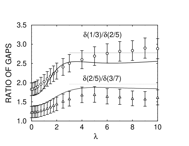
FIG. 2.: Ratios of excitation gaps at filling fractions 1/3, 2/5 and 3/7. The points are the calculations from the CF wave functions and the lines from the MS formulas. The horizontal lines depict the asymptotic $\lambda\rightarrow\infty$ limit of the MS ratio.

We note that earlier work[8, 24] found that the gaps at $\lambda=0$ scale approximately as

$$\Delta=C\frac{e^{2}}{l}\frac{1}{(2p+1)}\;,$$ (17)

which implies that

$$\Delta\propto[p(2p+1)]^{-1/2}\;.$$ (18)

A comparison with Eq. (11) shows that the gaps at large $\lambda$ should decrease faster with $p$ than the ones at $\lambda=0$. Another interesting implication is regarding the effective mass of composite fermions, $m^{*}$, which is obtained by equating the gaps to the CF cyclotron energy $eB^{*}/m^{*}=eB/(2p+1)m^{*}$. While at $\lambda=0$ one would expect $m^{*}\sim\sqrt{(2p+1)/p}\sim\sqrt{B}$, at large $\lambda$, Eq. (11) implies $m^{*}\sim(2p+1)^{2}/p$, which has a much stronger dependence on the filling factor, diverging as $\nu\rightarrow 1/2$. These results are generally consistent with the trends found in the gaps computed from the CF wave functions[23].

Now we turn to Scaling Relation II, Eqn.(16). Fig. 3 shows the scaling prediction for the gaps at $p/(4p+1)$, [which requires the gaps at $p/(2p+1)$ as input], along with the gaps at $p/(4p+1)$ computed directly from the CF wave functions. For large values of $\lambda$, the two gaps are in agreement within numerical uncertainty. But they are very close even for small $\lambda$, which is unexpected in the formalism aimed at the infrared.

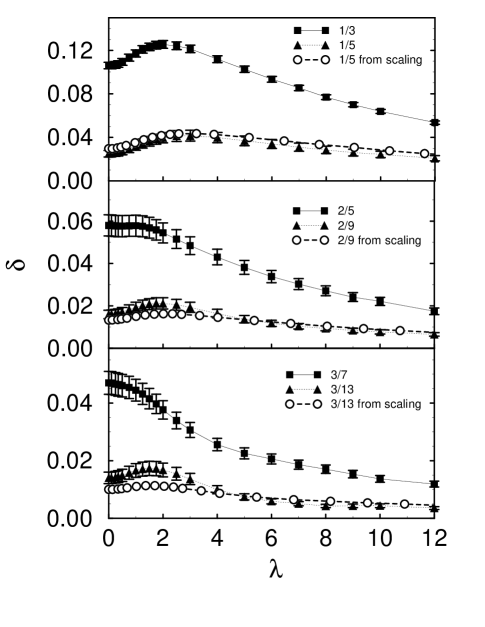
FIG. 3.: The gaps for several FQHE states at $p/(2p+1)$ and $p/(4p+1)$ computed from the CF wave functions for the model interaction potential $v(r)$. The circles show gaps at $p/(4p+1)$ deduced from the gaps at $p/(2p+1)$ using the scaling relation discussed in the text.

In hindsight, one can motivate the above scaling of gaps at corresponding fractions as follows. It has been noted before[25] that the charge density profiles of the particle or hole excitations at $p/(2sp+1)$ are largely independent of $s$, when plotted in terms of $l^{*}$. The main difference is that the total integrated charge is $e^{*}=e/(2sp+1)$. Therefore, it is natural to expect that the excitation energy is proportional to $e^{*2}/l^{*}$. (The constant of proportionality will clearly depend on $p$, since the density profiles of of the excitations depend strongly on $p$, but may be expected to have only a weak dependence on $s$). This is precisely the above scaling relation. While the argument is very natural, it not trivial to derive it systematically within the theory.

We have neglected the possibility that the FQHE become unstable at large thicknesses, as found in numerical studies[26]. This physics is not relevant to our main concern here, which is to test the consistency of the MS approach.

In conclusion, we have tested functional relations between the gaps coming out of the Hamiltonian approach of Murthy and Shankar, and found them to be in good agreement with the results obtained from the CF wave functions. G.M. thanks Andy Millis and R.S thanks N. Read for stimulating conversations. We are grateful for support from the NSF grants no. DMR98-00626 (RS) and DMR-9615005 (JKJ) and a grant of computing time on the SGI Power Challenge cluster at the NCSA, University of Illinois, Urbana-Champaign.

REFERENCES

- [1] D.Tsui, H.Stromer and A.Gossard, Phys. Rev. Lett. 48, 1599, (1982).
- [2] J.K.Jain, Phys. Rev. Lett. 63, 199, (1989); Phys. Rev. B 41, 7653 (1990); Science 266, 1199 (1994).
- [3] J.K. Jain and R. Kamilla, to appear in “Composite Fermions”, Olle Heinonen, Editor; Int. J. Mod. Phys. B 11, 2621 (1997).
- [4] S.Deser, R.Jackiw and S.Templeton, Phys. Lett. B139, 371 (1982).
- [5] S.M. Grivin and A.H. MacDonald, Phys. Rev. Lett. 58, 1252 (1987); S.-C.Zhang, H.Hansson and S.A.Kivelson, Phys. Rev. Lett. 62, 82, (1989); N.Read, Phys. Rev. Lett., 62, 86 (1989).
- [6] A. Lopez and E.Fradkin, Phys. Rev. B 44, 5246 (1991), ibid 47, 7080, (1993), Phys. Rev. Lett. 69, 2126 (1992).
- [7] V.Kalmeyer and S.-C.Zhang, Phys. Rev.B46, 9889 (1992).
- [8] B.I.Halperin, P.A.Lee and N.Read, Phys. Rev. B47, 7312 (1993).
- [9] R.Shankar and G.Murthy, Phys. Rev. Lett. 79, 4437, (1997).
- [10] G.Murthy and R.Shankar, to appear in “Composite Fermions”, Olle Heinonen, Editor (cond-mat 9802244).
- [11] G.Murthy and R.Shankar, cond-mat 9806380.
- [12] D. Bohm and D. Pines, Phys. Rev. 92, 609, (1953).
- [13] S.H.Simon, A.Stern, and B.I.Halperin, Phys. Rev. B54, R11114 (1996).
- [14] W.Kohn, Phys. Rev 123, 1242 (1961).
- [15] S.M.Girvin, A.H. MacDonald and P. Platzman, Phys. Rev. B33, 2481, (1986).
- [16] R. B. Laughlin, Phys. Rev. Lett.50, 1395, (1983).
- [17] N.Read Semi. Sci. Tech. 9, 1859 (1994).
- [18] D.H. Lee, Phys. Rev. Lett.80, 4745 (1998).
- [19] V.Pasquier and F.D.M.Haldane, cond-mat 9712169.
- [20] N.Read, cond-mat 9804294.
- [21] F.C.Zhang and S. Das Sarma, Phys. Rev. B 33, 2903 (1986); D.Yoshioka, J. Phys. Soc. Jpn. 55, 885 (1986).
- [22] B.I.Halperin and A.Stern, Phys. Rev. Lett.80, 5457 (1998); G.Murthy and R.Shankar, Phys. Rev. Lett.80, 5458 (1998).
- [23] K. Park and J.K. Jain, preprint.
- [24] J.K. Jain and R.K. Kamilla, Phys. Rev. B 55, R4895 (1997).
- [25] R.K. Kamilla, X.G. Wu, and J.K. Jain, Phys. Rev. B 54, 4873 (1996).
- [26] F.D.M. Haldane and E.H. Rezayi, Phys. Rev. Lett. 54, 237 (1985).