Low-temperature properties of classical, geometrically frustrated antiferromagnets

Abstract

We study the ground-state and low-energy properties of classical vector spin models with nearest-neighbour antiferromagnetic interactions on a class of geometrically frustrated lattices which includes the kagome and pyrochlore lattices. We explore the behaviour of these magnets that results from their large ground-state degeneracies, emphasising universal features and systematic differences between individual models. We investigate the circumstances under which thermal fluctuations select a particular subset of the ground states, and find that this happens only for the models with the smallest ground-state degeneracies. For the pyrochlore magnets, we give an explicit construction of all ground states, and show that they are not separated by internal energy barriers. We study the precessional spin dynamics of the Heisenberg pyrochlore antiferromagnet. There is no freezing transition or selection of preferred states. Instead, the relaxation time at low temperature, $T$, is of order $\hbar/k_{B}T$. We argue that this behaviour can also be expected in some other systems, including the Heisenberg model for the compound $SrCr_{8}Ga_{4}O_{19}$.

]

I Introduction

Experimental and theoretical studies in recent years have found that geometrically frustrated antiferromagnets display properties quite unlike those of other magnetic systems.[1] These materials have magnetic ions located on lattices of site-sharing frustrated units - usually triangles or tetrahedra. One of the best-studied systems in this class is the layered compound $SrCr_{8}Ga_{4}O_{19}$ ($SCGO$).[2, 3, 4, 5, 6, 7, 8, 9, 10] Attention has focussed on the fact that the majority of its magnetic $Cr^{3+}$-ions reside on the sites kagome lattices, although the full structure is more complex. Following the interest in kagome magnets generated by studies of $SCGO$, a great deal of attention has been devoted to the oxide and fluoride pyrochlore magnets, in which the magnetic ions form a lattice of corner-sharing tetrahedra as depicted in Fig. 1. Neutron scattering[4, 6, 7, 8, 9, 10, 11, 12, 13, 14, 15, 16, 17] and muon spin relaxation[18, 19, 20] experiments on $SCGO$ and the pyrochlores have detected only short-range magnetic correlations and a slowing-down of fluctuations at low temperatures.[1] More generally, it is apparently a characteristic property of geometrically frustrated magnets that they do not order at the temperature expected from the magnitude of the Curie-Weiss constant, $|\Theta_{CW}|$. Instead they remain in the paramagnetic phase to a much lower temperature with - typically - spin freezing at $T_{F}\ll|\Theta_{CW}|$.[21, 22, 23]

A detailed understanding of the origin of such generic features has been slow to emerge. Moreover, there has been little work to explain systematic differences between individual examples of these magnetic systems. For instance, whereas in the Heisenberg kagome antiferromagnet thermal fluctuations give rise to entropic ground-state selection,[24, 25] known as order by disorder,[26, 27, 28, 29, 30] this phenomenon appears to be absent for some related systems.[31, 32] The reason for the difference is unclear, as are the general conditions under which such selection should be expected for geometrically frustrated magnets. In this context, it is interesting to ask whether $SCGO$ inherits its properties from those of the kagome Heisenberg antiferromagnet, or whether its behaviour is closer to that of the pyrochlore antiferromagnet, since an alternative and more complete description of the structure is to regard a layer of $SCGO$ as a slab cut from the pyrochlore lattice, consisting of three consecutive [111] lattice planes.

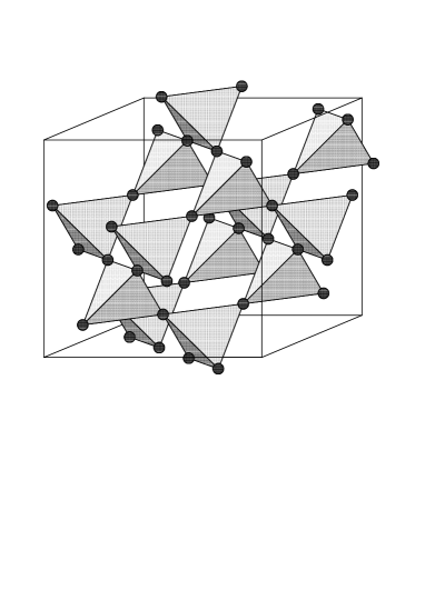
FIG. 1.: The pyrochlore lattice

A further area for investigation, in addition to the statistical mechanics of geometrically frustrated antiferromagnets, is their low-temperature dynamics, which has so far received only limited attention.[33, 34] Dynamical correlations are likely to be profoundly influenced by the large ground state degeneracy of these systems, and constitute one of their most interesting aspects.

In an attempt to extend understanding of these problems, we have studied the low-temperature properties of the classical Heisenberg model with nearest-neighbour interactions on a class of geometrically frustrated lattices. This description neglects various additional features – such as anisotropy,[35, 36, 37, 38, 39] disorder,[40] dipolar[41] or further-neighbour interactions,[42, 43] and quantum effects[25, 44, 45, 46, 47, 48, 49, 50] – which can play an important role in real materials, particularly near and below $T_{F}$. However, it may provide a good treatment for the temperature window $T<T_{F}\ll|\Theta_{CW}|$, and its simplicity should make it well-suited for capturing the generic features of these systems, as well as providing a basis for future investigations incorporating additional interactions or quantum fluctuations.

Our work, parts of which have been described in Refs. [51] and [52], concentrates on the pyrochlore antiferromagnet, but we address several questions in a more general context. We start by analysing the origin and extent of the ground-state degeneracy of geometrically frustrated magnets (Sect. II). We discuss the nature of the ground-state manifold of pyrochlore antiferromagnets with $n$-component spins (Sect. III). We give an explicit construction of all ground states of these magnets, and show that they are not separated by energy barriers. Although typical ground states are disordered, we show that certain correlations remain, which give rise to distinctive features in magnetic neutron scattering. We study, both analytically (Sect. IV) and numerically (Sect. V), the existence of order by disorder for a general class of geometrically frustrated antiferromagnets and find that it occurs only for magnets with small ground-state degeneracies. In particular, it is absent from the Heisenberg pyrochlore magnet, which therefore has neither internal energy nor large free energy barriers separating different ground states. Because of this, the system is not trapped near a particular state at low temperatures. Our study of the precessional dynamics at low temperatures and for long times (Sect. VI) reveals that the decay of the autocorrelation function is exponential in time, $t$, with a timescale inversely proportional to the temperature and independent of the exchange energy: $\langle{\bf S}_{i}(0).{\bf S}_{i}(t)\rangle=\exp(-ck_{B}Tt/\hbar)$, where $c$ is ${\cal O}(1)$. In agreement with Reimers’ earlier Monte Carlo simulations, [33] we find that the spin-freezing transition observed experimentally does not happen in the simple Heisenberg model we consider. We discuss recent experiments on pyrochlore magnets[16] and $SCGO$[7, 10] in the light of these results.

Since spin correlations are short-ranged in both space and time, the Heisenberg pyrochlore antiferromagnet can be labelled a classical spin liquid or, following Villain,[53] a cooperative paramagnet.

II The Heisenberg spin Hamiltonian on geometrically frustrated lattices

Consider $n$-component classical spins, ${\bf{S}}_{i}$, with $|{\bf{S}}_{i}|=1$, arranged in corner-sharing units of $q$ sites. Each spin is coupled antiferromagnetically with its $q-1$ neighbours in each unit, so that the Hamiltonian is

$$H = J\sum_{<i,j>}{\bf{S}}_{i}\cdot{\bf{S}}_{j}\equiv\frac{J}{2}\sum_{\alpha}|{\bf L}_{\alpha}|^{2}-~{}\frac{J}{2}Nq.$$ (1)

Here, $J$ is the exchange constant and ${\bf L}_{\alpha}$ is total spin in unit $\alpha$. The sum on $\left<i,j\right>$ runs over all neighbouring pairs and the sum on $\alpha$ runs over the $N$ units making up the system.

Note that our motivation for considering $n$-component spins is to shed light on the systematics of geometrically frustrated antiferromagnets. Because of this, we take the $n$-component spin-space to be the same at each site. Of course, the case $n=2$ can also arise physically in a Heisenberg system with easy-plane anisotropy: in this event, which has been studied in Ref. [54], the easy planes are orientated differently at different sites, in accordance with the local symmetry axes.

An instructive way of thinking about the strength of the geometric frustration is to consider the extra ground-state degeneracy which it gives rise to, in addition to that stemming from the symmetry of the Hamiltonian. It is this extra degeneracy which lies behind many of the physical properties peculiar to geometrically frustrated systems. To determine the number, $D$, of degrees of freedom in the ground state, we use a Maxwellian counting argument, [42, 55] and evaluate $D_{M}\equiv F-K$, the difference between the total number, $F$, of degrees of freedom in the system, and the number, $K$, of constraints that must be imposed to restrict the system to its ground states. In general, as discussed below, $D_{M}\not=D$, but for pyrochlore antiferromagnets we argue in Sect. III B that $D_{M}/D\to 1$ as $N\to\infty$.

To evaluate $K$, note that, from Eq. 1, a configuration is a ground state provided ${\bf L}_{\alpha}=0$ for each unit separately. This imposes $Nn$ constraints. To find $F$, we start from the fact that the number of degrees of freedom is simply $n-1$ per spin. Expressed in terms of the number, $N$, of units, $F$ depends on their geometric arrangement. For corner-sharing units of $q$ spins, $F=Nq(n-1)/2$. Alternative arrangements generally result in smaller values of $F/N$ and in ground states that are not extensively degenerate. For example, if bonds are shared between units – as in the triangular and face-centred cubic lattices for $q=3$ and $q=4$ respectively – $F$ is lower than if only sites are shared – as in the kagome and the pyrochlore lattices – since each spin belongs only to $b=2$ units in the latter case but to more ($b=6$ and $8$, respectively) in the former. In the general case, we obtain $F=Nq(n-1)/b$. Hence, $D_{M}/N=\left[q(n-1)/b-n\right]$. $D_{M}$ grows with $q$ and, for $q>b$, with $n$. In order to obtain $D_{M}>0$, we require $q>b$, which is the case only for corner-sharing arrangements. The physically realisable example for which $D_{M}$ is maximal is that for which $q$ and $n$ are both maximal: Heisenberg spins ($n=3$) on the pyrochlore lattice ($q=4$) represent the only simple system for which $D_{M}$ is positive and extensive. It is partly for this reason that the pyrochlore Heisenberg antiferromagnet is particularly interesting.

This counting argument can go wrong in two ways. Firstly, the $K$ constraints may not be independent, as happens for Heisenberg spins on the kagome lattice, where $D_{M}=0$ but an extensive ground-state degeneracy nonetheless arises. Secondly, for some lattices there may be no spin configurations that satisfy the conditions ${\bf L}_{\alpha}=0$ for all $\alpha$.

Many of the results presented in this paper do not depend on the details of the lattice under consideration but rather on the size $q$ of the corner-sharing units. We find it useful to consider, in addition to the pyrochlore lattice, the two-dimensional square lattice with crossings[56] (Fig. 2), which is not known to occur in nature but is easy to visualise. Like the pyrochlore lattice, from which it can be obtained by a projection in a $\left<001\right>$ direction, it has $q=4$  and, with Heisenberg spins, $D_{M}=N$.

FIG. 2.: The square lattice with crossings. Both solid and broken lines denote exchange interactions. Spins reside on the intersections of the solid lines.

Also, more complicated corner-sharing arrangements of frustrated units are possible. Of particular experimental importance, as mentioned above, is the combination of triangles and tetrahedra found in $SCGO$, which is depicted in Fig. 3.

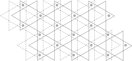
FIG. 3.: Projection of the sites of the magnetic $Cr^{3+}$ ions in one layer of SCGO. The ions occupy sites of the kagome lattices in the top (solid lines) and bottom (dashed lines) planes. In the middle plane, the ions are located on a triangular lattice (indicated by circles). All lines denote exchange interactions; there are also interactions between a spin in the middle plane and those in the two triangles which enclose it.

III The ground states of classical antiferromagnets on the pyrochlore lattice

It has been realised for a long time that antiferromagnets on the pyrochlore lattice have a vast ground-state degeneracy,[57, 53] but no explicit construction of the ground states has as yet been available. The nature of various submanifolds of the ground-state manifold is however known. These submanifolds are defined by imposing extra constraints on the spin arrangement, in addition to the requirement that it be a ground sate. A simple example is the set of four-sublattice states, in which the four spins of each unit cell are arranged to be oriented the same way everywhere. Any four-spin arrangement that is a ground state for the single tetrahedron (see section III A) yields a ground state for the entire system by periodic repetition. Of these states, those with two spins parallel and two antiparallel to a given axis are the simplest conceivable ones. Villain[53] has described a larger ground-state submanifold for the Heisenberg model, in which the spins of each tetrahedron form two antiparallel pairs. It turns out that for $XY$ model all ground states are of this kind, as described in Sect. III E.

In the following, we present complete constructions of the ground states for classical antiferromagnets with $n$-component spins on the pyrochlore lattice. We also show that the ground-state manifold is connected. We then examine the conequences of spin correlations in typical ground states for elastic neutron scattering. We conclude this section with a discussion of the nature of the ground-state degrees of freedom in such magnets.

A The single tetrahedron

The ground states of a single tetrahedron are those states in which the sum, ${\bf L}$, of the four spin vectors has the value ${\bf{L}}=0$. In such a configuration, any two spins enclose the same angle as the other two. For Heisenberg spins, these configurations can be parametrised by two coordinates (e.g. $a$ and $\phi$ in Fig. 4). The crucial feature is that, for any fixed $a$ except $a=0$, one can choose $\phi$ independently. In the special case, $a=0$, if spins 1 and 4 are antiparallel, there are two degrees of freedom associated with the remaining two spins, while if spins 1 and 4 are parallel, there is no remaining freedom. These exceptional states, in which all spins of a tetrahedron are collinear, can play a central role in determining the thermodynamics of the system because they are favoured by thermal fluctuations, as discussed in section IV A.

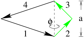
FIG. 4.: Four spins of equal length with vector sum ${\bf L}=0$. Spins 1 and 4 lie in the plane of the paper, spins 2 and 3 need not.

For the $XY$ antiferromagnet, there is only one continuous degree of freedom, $a$, since if spins are coplanar, $\phi=0,\pi$. Ground states are therefore the configurations with two pairs of antiparallel spins.

B The Heisenberg antiferromagnet

1 The construction of the ground states

We give in this subsection a stepwise procedure for constructing any ground state of the Heisenberg pyrochlore antiferromagnet, from which the number of ground-state degrees of freedom, $D$, can be determined directly. We also consider a similar proceedure for the square lattice with crossings since it is essentially the same but easier to explain and visualise. The idea in both cases is that the ground state can be built up by choosing the orientations of spins on successive layers (planes or lines) of the lattice, in a way that requires no adjustments of spins in planes or lines already visited. We consider systems with open boundary conditions: in the context of this section, periodic boundary conditions appear to introduce significant additional mathematical difficulties.

We define a layer, for the square lattice with crossings, to be a [10] plane (Fig. 5), and for the pyrochlore lattice to be a [100] plane. In both cases, a layer contains the spins lying on equivalent edges of squares or tetrahedra – referred to as units from hereon – which are next-nearest, but not nearest, neighbours, to other units with spins in the layer. The spins of each unit are shared between two adjacent layers. Conversely, each spin belongs to a unit extending above and one extending below the layer.

First, choose the orientations of the spins on the lowest layer of the lattice. This amounts to choosing a value for $a$ in each unit with spins on the bottom layer. There are no restrictions on how to do this. Next, consider the adjacent layer: when choosing the orientation of spins on that layer, one has to satisfy the ground-state condition. For each unit, this leaves one degree of freedom, $\phi$, except in the special case, $a=0$. For this special case, one has to distinguish two situations. If the bottom spins of a unit are antiparallel, there are two degrees of freedom when choosing the ground state orientation of the upper pair of spins: when counting ground-state coordinates, the loss of a coordinate that follows from the additional constraint, $a=0$, is exactly balanced by the gain of an additional degree of freedom for the upper pair of spins. In the alternative situation, in which the first pair of spins is parallel, no freedom remains, and we obtain a lower-dimensional submanifold of the ground state.

At this stage, we have fixed the orientation of spins in the lowest two layers of the lattice. Repeating the procedure in the subsequent layers, the value for $a$ in each unit is determined by earlier choices, while one degree of freedom, $\phi$, remains for each unit of the system.

Since any given ground state can be built up (or copied) layer by layer in this way, the construction can be used to generate all possible ground states. By this construction we have demonstrated that the extensive part of the dimension of the ground-state manifold is equal to the number of units in the system.

2 The connectedness of the ground-state manifold

We show that the ground-state manifold is connected by demonstrating that any ground state can be continuously deformed into any other ground state without cost in energy. To do so, we choose a reference ground state and give an explicit construction by which the reference state can be reached from any ground state, without leaving the ground state manifold. This is done by considering successive layers of the system, and bringing the spins in each layer into the orientation that they have in the reference state, using moves within the ground-state manifold which leave spins unchanged in the layers already visited. The reference state is chosen to be one in which all spins on lattice sites equivalent under translation have the same orientation, and in which each spin is antiparallel to the other spin belonging to the same layer and unit.

FIG. 5.: When altering the orientation of the spins represented by empty circles, only spins inside the wedge defined by the fixed spins (filled circles) have to be adjusted. For the pyrochlore lattice, a cone replaces the wedge.

We make use of the following facts, which follow straightforwardly from consideration of the ground-state configurations illustrated in Fig. 4:

(I) For a single unit of four spins, the manifold of ground states is connected: $a$ and $\phi$ (Fig. 4), which provide a complete parametrisation of the internal degrees of freedom of the ground-state manifold, can be chosen independently from intervals of the real axis. Moreover, the orientation of any two chosen spins can be changed arbitrarily and continuously without leaving the groundstate manifold, as long as the other two spins are unconstrained.

(II) If two spins in a unit are antialigned, so will be the other two, whose common axis can then be rotated arbitrarily and continuously while keeping the orientation of the first pair fixed and remaining in the ground-state manifold.

(III) It is possible to change the orientation of one spin in a unit arbitrarily and continuously while that of a second is held fixed, without leaving the ground-state manifold, as long as the other two spins are unconstrained. This is a special case of (I).

(IV) From II and III it follows that one can continuously change the orientation of a pair of spins belonging to a unit in the bottom layer, or a pair of antiparallel spins in a higher layer, and remain within the ground-state manifold of the whole system, whilst keeping fixed the spins that lie outside a wedge (or cone) for the square lattice with crossings (or the pyrochlore lattice), as depicted in Fig. 5.

As a consequence, we can again work through the lattice layer by layer. The procedure is as follows.

(A) Align the spins in the bottom layer, unit by unit, to coincide with the reference state. This fixes the two spins of each unit in the bottom layer to be antiparallel. As we adjust the orientation of spins in the lower layer of each unit, those in the upper layer of the same unit can, by I, be reorientated to keep the unit always in a ground state. At the same time, by IV, spins in higher layers can also be reorientated to keep the system as a whole in a ground state.

At this stage, spins in the bottom layer are in their reference state.

(B) Spins in the second layer now form antiparallel pairs, since they belong to units which have antiparallel pairs in the lowest layer. The spins in the second layer can therefore, by II, be adjusted to coincide with those in the reference state. While this is done, by IV, spins in higher layers can be concurrently reorientated to keep the system within a ground state, as in step A.

From the way we chose the reference state, it now follows that all neighbouring spins in the second layer are pairwise antiparallel. Therefore, we can repeat step B for the third and all higher layers. Once we have done so, all spins in the system coincide with those in the reference state. Since one can go between two arbitrary ground states via the reference state, this completes our proof that the ground state manifold is connected.

C Pyrochlore antiferromagnets with general $n\geq 2$

The arguments presented in the previous section for Heisenberg antiferromagnets generalise directly to $n$-component spins with $n>3$. For the ground-state construction, the main difference is that spins 2 and 3 in Fig. 4 can now be rotated in $n-2$ directions, so that the extensive part of $D$ is $N(n-2)$, as expected from Maxwellian counting.

The construction of ground states for the $XY$ model is much simpler than for the Heisenberg model: as in the case of a Heisenberg antiferromagnet on the kagome lattice, for a generic ground state the number of constraints is equal to the total number of degrees of freedom. The construction of the ground states therefore involves fewer choices. It proceeds as follows. The orientations of spins in the bottom layer can be chosen arbitrarily. The ground-state configurations of spins in the next layer are then almost completely determined, since each tetrahedron has two pairs of antiparallel spins. The only freedom remaining is the discrete choice of which spin to place on which of the two sites of the unit in the next layer, unless the two spins of a unit in the lower layer happen to be antiparallel. In this case the orientation of the pair (which has to be antiparallel) in the top layer be chosen freely.

The proof of the connectedness of the ground-state manifold, presented above, follows essentially from the connectedness of the ground-state manifold of a single unit and from the fact that for any orientation of a pair of spins in a unit, the other pair can be chosen so that the total spin of the unit vanishes. This, along with the other steps, carries over to the case $n\geq 2$.

D Ground-state correlations of the Heisenberg pyrochlore antiferromagnet

It is clear in our construction of ground states that spin correlations are not propagated efficiently. In this section, we show that, nonetheless, a few long-range correlations in high-symmetry directions are built into the ground states of the pyrochlore Heisenberg antiferromagnet. We discuss the signatures of these correlations in magnetic neutron diffraction.

1 Correlations between planes

From the ground-state condition, ${\bf{L}}_{\alpha}=0$, it follows that the sum of all the spin vectors in two adjacent (100) planes is zero (this sum is also the sum of ${\bf{L}}_{\alpha}$ over tetrahedra making up the two planes). Therefore, adjacent planes are antiferromagnetically correlated. Since these correlations are long ranged, we expect sharp peaks in the neutron scattering cross section in the $\left<200\right>$ directions.

These peaks differ from Bragg peaks in two ways. First, their amplitude scales differently with sample size. Consider a sample in the form of a cube of side $L$, and let the total magnetisation of a (100) plane be $M$. In a typical ground state, $M\sim L$ and the peak scattering amplitude varies as $M\cdot L\sim L^{2}$, in contrast to $L^{3}$ for a Bragg peak. Second, they are sharp in only one direction in reciprocal space. Consider scattering at a point displaced from $(200)$ by the vector $(q_{\parallel},{\bf q}_{\perp})$. We argue that, at fixed ${\bf q}_{\perp}$, the scattering amplitude as a function of $q_{\parallel}$ has a peak centered on $q_{\parallel}=0$, of width $\delta q_{\parallel}\propto|{\bf q}_{\perp}|$. Contours of constant scattering intensity therefore have a distinctive bow-tie shape. To understand in detail the reason for this, it is necessary to examine the correlation in the magnetisation, $\cal{M}$, of a region of a $(100)$ plane with linear size $\cal{L}$, and that of its equivalent, displaced by a distance $z$ in the $[100]$ direction. Let $\delta{\cal M}_{z}$ be the difference between these magnetisations, and measure $z$ in units of the plane spacing. The magnetisation difference for adjacent planes, $\delta{\cal M}_{1}$, arises entirely from spins belonging to tetrahedra that are only partially included in the region. The number of such spins is proportional to the size of the boundary of the region – and hence to $\cal{L}$. Since there are only weak correlations between individual spins on distances larger than the size of a tetrahedron, we obtain $\delta M_{1}\propto\sqrt{\cal{L}}$. Increasing $z$, $\delta{\cal M}_{z}$ follows a random walk: $\delta{\cal M}_{z}\propto\sqrt{z}\sqrt{\cal{L}}$. Since $\cal{M}\sim\cal{L}$, we obtain a correlation length $\xi\propto\cal{L}$, and therefore $\delta q_{\parallel}\propto|{\bf q}_{\perp}|$.

Similarly, there are long-range correlations in the $\left<111\right>$ directions. The $\{111\}$ planes are alternately kagome and triangular planes. Adjacent kagome planes contain the bases of adjacent tetrahedra, which, in the intervening triangular planes, share a common apex. In any ground-state, the total magnetic moments of all (100) kagome planes are equal, and also opposite to the total magnetic moment of all (100) triangular planes.

2 Consequences for neutron scattering experiments

In recent neutron scattering experiments on a single crystal sample of $CsNiCrF_{6}$ by Harris et al.,[15, 58, 17] the angular dependence of the neutron scattering cross section is studied. The correlation length is longest in the $\left<100\right>$ direction, shortest in the $\left<110\right>$ direction, and intermediate in the $\left<111\right>$ direction. Since the presence of two species of magnetic ions in $CsNiCrF_{6}$ makes a detailed comparison with theory difficult, Harris et al. also report Monte Carlo studies [58, 17] of the angular neutron scattering cross section in the $\left[hhl\right]$ plane, shown in Fig. 6, which is taken from Ref [58].

The scattering is broad in most directions except the $[100]$ and $[111]$- directions, where narrow necks appear at low temperature. The scattering near these necks has the appearance of a bow-tie, as described above. In addition to these bow-ties, which are narrow in the direction parallel to the wavevector transfer, there are subsidiary bow ties, narrow in a perpendicular direction. Their origin can also be explained using arguments of the kind described above.

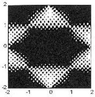
FIG. 6.: Static neutron scattering cross section in the $[hhl]$ plane for a Heisenberg pyrochlore antiferromagnet, obtained numerically by quenching the system into a ground state. Horizontal and vertical coordinates are $l$  and $h$ respectively. Light shaded areas represent high intensity, and black represents zero intensity.

E Local zero modes

We next discuss the existence of degrees of freedom in the ground state which involve only spins in a finite region in the bulk of the system. These we call local zero modes. They are of interest because unhindered rotation of finite numbers of spins is likely to be particularly effective at destroying correlations, both in space and in time.

In the kagome magnet, the nature of the zero modes was established in Refs. [24] and [25]. The requirement that ${\bf{L}}=0$ leads the three spins in each triangle to be coplanar and at relative angles of $120^{\circ}$. If all the spins on the lattice are coplanar, there are three spin orientations, ($A,B,C$), each of which occurs in each triangle once. A zero mode, called a weathervane defect,[25] arises as follows. In a region enclosed by a line of spins of one type (say, $C$), a line of spins (alternating between type $A$ and $B$) can be rotated about the spin direction of $C$ at no cost in energy. Starting from a particular state, any ground state can be constructed using these zero modes.[24, 59]

There is a closely related way of describing the zero modes for the $XY$ magnet on the pyrochlore lattice. They are again associated with closed loops, this time of antiferromagnetically oriented spins. Our construction of a ground state in section III amounts to finding a set of lines through the lattice sites with adjacent sites on a line occupied by antiparallel nearest neighbour spins, and each site belonging to exactly one line. Each line can be labelled with an angle giving the orientation of its spins, and a zero mode involves changing one such angle. Villain[53] used a description of this kind to generate a subset of the ground states of the Heisenberg pyrochlore antiferromagnet. By contrast, for the $XY$ model, this approach generates all the ground states.

For the Heisenberg antiferromagnet on the pyrochlore lattice, the nature of the zero modes is much more complicated, reflecting the larger freedom in the ground-state manifold. We have not been able to find a simple description of a generic zero mode. We nevertheless believe that in a sufficiently large region of a generic ground state, there are local zero modes. Our argument rests on counting degrees of freedom: the number of degrees of freedom a region contributes to the ground state is proportional to its volume, while fixing surrounding spins imposes a number of constraints proportional to its surface. For a large enough volume, the number of degrees of freedom exceedes the number of such constraints. The existence of such local modes in all ground states is however not guaranteed. For instance, for a state in which all spins in a given $\left(001\right)$ plane are parallel, and antiparallel to the spins in neighbouring planes, the sum rules discussed in section III D preclude the existence of local zero modes.

IV Ground-state selection at low temperatures: analytical results

In this section, we examine the circumstances under which thermal fluctuations induce order in geometrically frustrated antiferromagnets. This phenomenon – known as order by disorder – has been discussed in great detail for the Heisenberg antiferromagnet on the kagome lattice, where thermal fluctuations induce coplanar ordering of the spins.[24, 25, 59] There is evidence from past simulations that order by disorder is not a universal occurrence in geometrically frustrated systems – both Heisenberg spins on the pyrochlore lattice [33, 58] and four-component spins on the kagome lattice [31] apparently remain disordered at low temperature – but the systematics have not previously been studied.

The experimental situation for pyrochlore magnets is rather complicated. A few compounds develop long-range order at low temperatures,[35] whereas others undergo a spin-glass transition.[23] It is unclear what the importance is of various features of real systems. Nevertheless, we restrict our attention in the following to the theoretically idealised problem of a classical antiferromagnet, without anisotropy, disorder, further-neighbour or dipolar interactions.

This material is arranged as follows. First, we consider the analytically accessible problem of four Heisenberg or $XY$ spins on a single tetrahedron. Next, we investigate the general case of a lattice built from groups of $q$ spins, each with $n$ components, and ask whether thermal fluctuations restrict the spins to an ordered (e.g. collinear or coplanar) configuration. Then, in Sect. V, we present the results of numerical simulations, which test the conclusions reached from our analytical arguments.

A The single tetrahedron

We first study a problem simple enough to allow explicit evaluation of some of the quantities of interest: antiferromagnetically coupled spins occupying the corners of an isolated tetrahedron.

There are eight degrees of freedom associated with four Heisenberg spins, and for the system to be in a ground state, three constraints must be satisfied, since ${\bf{L}}=0$. The ground state manifold therefore has five dimensions: of these, three arise from global rotations, while the remaining two can be parameterised as discussed in Sect. III A. The energy cost for fluctuations from this ground-state manifold in the remaining three directions in configuration space is, for a generic ground state, quadratic in displacement. By contrast, for the special ground states in which spins are collinear, energy varies quadratically with displacement from the ground state manifold only in two directions, and quartically in the third, indicated schematically in Fig. 7. The collinear states are the obvious candidates for selection by thermal fluctuations.

FIG. 7.: Soft fluctuations around a collinear state

To study such selection, we have calculated the probability distribution, $W(\theta)$, for the angle, $\theta$, between a pair of Heisenberg spins, integrating over all orientations of the four spins with a Boltzmann distribution and the Hamitonian of Eq. 1. Two factors contribute to $W(\theta)d\theta$: the measure, $\sin(\theta)d\theta$, and a statistical weight. The low-temperature limit of the latter is $[2\cos(\theta/2)]^{-1}$, the divergence as $\theta\to\pi$ reflecting the lower free energy attached to fluctuations around the collinear state. Combining both factors, $W(\theta)=\sin(\theta/2)d\theta/2$: configurations which are nearly collinear have higher weight than others in this distribution, but the entire ground-state manifold is accessible even in the low-temperature limit, and there is no fluctuation-induced ground-state selection.

To illustrate the alternative, consider the same problem for $XY$ spins. In this case, the measure contributes simply $d\theta$ to the distribution, $W(\theta)d\theta$, while the statistical weight at temperature $T\ll J$ is proportional to $|\sin(\theta)|^{-1}$ for $\sin^{2}(\theta)\gg T/J$, and to $(J/T)^{1/2}$ for $\sin^{2}(\theta)\ll T/J$. As a result, the weight in the limit $T\rightarrow 0$ is overwhelmingly concentrated near collinear spin arrangements ($\theta=0$ and $\pi$), reflecting selection of these states by thermal fluctuations. Order by disorder is just such a concentration of statistical weight on a submanifold of ground states. Note that it can occur in a finite system (in this case, a system of four spins), and is quite different from the order that appears in a symmetry-breaking phase transition, which is restricted to the thermodynamic limit.

It is straightforward to demonstrate these effects in Monte Carlo simulations. In Fig. 8, we plot the collinearity parameter, $P(1)$ (defined in section V A, Eq. 5), as a function of Monte Carlo time, for a simulation of four Heisenberg spins arranged in a single tetrahedron at the temperature $T=2.5\times 10^{-5}J$. For the current purposes, it is sufficient to note that the collinearity parameter takes on values between $-1/3$ (for a state with all spins at relative angles of $70.5^{o}$ or $109.5^{o}$) and $+1$ (when all spins are collinear). We see from Fig. 8 that the system explores all ground states, attaining values of the collinearity within $2\times 10^{-4}$ of the extremal ones, and is not trapped near a collinear state. The average of the collinearity parameter, $0.193\pm 0.02$, is distinct from $0$, its value in the high-temperature limit, and close to the exact low-temperature value, $1/5$, obtained from the expression for $W(\theta)$ given above.

FIG. 8.: Evolution of the collinearity parameter with Monte-Carlo time for a single tetrahedron at $T=2.5\times 10^{-5}J$ for $2\times 10^{7}$ Monte-Carlo steps per spin.

B The general problem: groups of $q$ spins with $n$ components

We now examine whether thermal fluctuations select particular ground states for the general class of system introduced in Sect. II, in which a lattice is built from $N$ corner-sharing units of $q$ spins, each having $n$ components. We have argued elsewhere [51] that low-temperature behaviour is characterised by a probability distribution over the ground-state manifold, defined in the limit $T\to 0$. Let ${\bf x}$ be coordinates on the ground-state manifold; at each point ${\bf x}$, one can introduce local coordinates, ${\bf y}$, spanning the remaining directions in configuration space. Generically, the energy of the system relative to its ground-state value will have a Taylor expansion with the leading term

$$H\approx H_{2}=\sum_{l}\epsilon_{l}({\bf x})y_{l}^{2},$$ (2)

resulting in a ground-state probability density

$$Z({\bf x})\propto\int d\{y_{l}\}e^{-\beta H_{2}}\propto\prod_{l}(k_{{\rm B}}T/\epsilon_{l}({\bf x}))^{1/2}.$$ (3)

In principle, order might arise in either of two ways. First, it can happen that certain, special ground states have soft fluctuations, so that at some point, ${\bf x}_{0}$, on the ground state manifold (or, more generally, on some subspace), some of the $\epsilon_{l}({\bf x}_{0})$ vanish. Then $Z({\bf x})$ will diverge as ${\bf x}$ approaches ${\bf x}_{0}$. If any such divergences are non-integrable, one should keep higher order terms from Eq. 2 when calculating $Z({\bf x})$. The result of doing so will be, in the limit $T\to 0$, a distribution concentrated exclusively on the subset of ground states for which $Z({\bf x})$ is divergent: these are the configurations selected by thermal fluctuations. It is this mechanism for fluctuation-induced order that we study. There is, however, also a second possibility, which we do not persue here: it might happen that the probability density, $Z({\bf x})$, is spread smoothly over the ground-state manifold, but that there nevertheless exist correlation functions which, when averaged with this weight, are long-ranged.

To decide whether ground states with soft modes are selected, it is necessary to know the number, $M$, of $\epsilon_{l}$ that vanish, and the dimension, $S$, of the subspace on which this happens. Close to this subspace, we separate ${\bf x}\equiv({\bf u},{\bf v})$ into an $S$-dimensional component ${\bf u}$, lying within the subspace, and a $(D-S)$-dimensional component ${\bf v}$, locally orthogonal to it, with magnitude $v$. We expect at small $v$ the behaviour $\epsilon_{l}({\bf x})\propto v^{2}$ for $M$ of the $\epsilon_{l}$’s. Hence, $Z({\bf x})$ diverges as $v^{-M}$ for small $v$, and the subspace is selected [51] as $T\to 0$ if the integral

$$\int Z({\bf u},{\bf v})d{\bf v}\,\propto\,\int v^{D-S-M-1}dv$$ (4)

is divergent at small $v$.

FIG. 9.: The occurence of order by disorder for $n$-component spins arranged in corner-sharing units, each consisting of $q$ spins. Ordered (marginal) models are denoted by circles (crosses).

We therefore need to consider candidate ordering patterns, and determine the sign of $D-S-M$ in each case. It seems in general that the preferred ground states are ones in which spins are collinear or coplanar, because these have the largest number of soft modes. Collinear spin order is possible on lattices built from units containing an even number of sites, $q$: in practice, those constructed from tetrahedra. Such order results in one soft mode per unit, as illustrated in Fig 7. The number of soft modes is therefore $M=N$, and (since $S=n-1$) we expect order only if $D<N$. Estimating $D$ as $F-K=N[q(n-1)-2n]/2$, we predict order if $n<(q+2)/(q-2)$, and disorder if $n>(q+2)/(q-2)$. Thus, for pyrochlore antiferromagnets, two-component spins order, and four-component spins do not. The approach reaches no conclusion in the marginal case of three-component spins, but simulations (Refs. [33, 58] and as described below) indicate that Heisenberg spins do not order. On lattices made from corner-sharing triangles, such as the kagome lattice, there are no collinear ground states; instead, coplanar order may occur. Such order results in $M=N/2$ soft modes;[24] using again the estimate $F-K=N[q(n-1)-2n]/2$ for $D$, we predict order in this case if $n<4$ and disorder if $n>4$. Simulations of kagome antiferromagnets demonstrate that there is indeed coplanar order for $n=3$,[24] and that the marginal case, $n=4$, is disordered.[31]

Summarising, the only cases in which there is order by disorder are $q=4,\ n=2$ (the $XY$ pyrochlore model) and $q=3,\ n=3$ (the Heisenberg kagome model). In both instances, there is a low entropic cost to enter the ordered state ($D_{M}=0$) and a high entropic gain from soft fluctuations because in the ordered state the constraints, ${\bf{L}}_{\alpha}=0$, are not independent. These conclusions are depicted in Fig. 9.

V Ground-state selection at low temperatures: numerical results

In the following two subsections, we present the results of the Monte Carlo simulations of $XY$ and Heisenberg pyrochlore antiferromagnets. One aim is to test our prediction of collinear ordering for $XY$ spins. We also consider the Heisenberg model in detail, to show that order by disorder is indeed absent in this case. Our studies of the Heisenberg antiferromagnet are a continuation of Reimers’ pioneering simulations [33] and Zinkin’s subsequent work.[58] Our conclusions are in agreement with these authors, in particular with the earlier – albeit tentative – ideas of Zinkin, but our results are more extensive. Reimers work concentrated on the temperature range $T\geq 0.05J$: many of the observations described in the following are very hard to discern or absent in this regime.

Our simulations were carried out on systems of sizes ranging from one unit cell ($N=2$ tetrahedra, $N_{s}=4$ spins) to $17^{3}$ unit cells ($N=9826,N_{s}=19652$). As pointed out in section IV, small systems display large fluctuations, and therefore require very long simulation runs. For $N_{s}=4$, the longest simulation was $2\times 10^{8}$ Monte Carlo steps per spin at $T=5\times 10^{-5}J$. For the largest system, however, only $1.5\times 10^{6}$ Monte Carlo steps per spin were necessary even at the lowest temperature.

A Correlation functions

In this subsection, we consider two-spin correlations and also a correlation function which quantifies directly the collinearity of the spin system. In the next subsection, we discuss the heat capacity, which is an indirect probe of the state of the system, but in some ways more conclusive, since it is sensitive to the presence of soft fluctuations irrespective of the type of ordering with which they are associated.

First, we demonstrate that the Heisenberg model does not have Néel order, even at low temperature. The correlation function $Q(r)\equiv\left<{\bf{S}}(0)\cdot{\bf{S}}(r)\right>$ is shown in Fig. 10: correlations are very small beyond the second neighbour distance. Second, to measure the collinearity of spins, we evaluate the correlation function (for $n$-component spins)

$$P(r)\equiv\frac{n}{n-1}\left(\langle\left({\bf{S}}(0)\cdot{\bf{S}}(r)\right)^{2}\rangle-\frac{1}{n}\right),$$ (5)

which is constructed to have the values $P=0$ at infinite temperature and $P=1$ in a collinear state. $P(r)$ is shown in Fig. 10, with $r$ in units of nearest-neighbour distances. The correlations for Heisenberg spins again have a range of only two nearest neigbour distances: there is no fluctuation-induced order. Equally, the predicted collinear order for $XY$ spins is confirmed: there is long-range order in $P(r)$ at this temperature. Note that, despite the very low temperature, the order parameter, $P(r\rightarrow\infty)\simeq 0.86$, is appreciably less than its maximum possible value of 1. We expect on general grounds that such nematic order should be established via a first-order phase transition, but have not attmepted to check this in detail in our simulations.

FIG. 10.: Correlation functions for the Heisenberg and $XY$ antiferromagnets at a temperature of $T=5\times 10^{-4}J$. The two-spin correlation function, $Q(r)$, (dot-dashed line) and the collinearity correlation function, $P(r)$, (solid line) for a system of 2048 Heisenberg spins; and $P(r)$ for a system of 864 $XY$ spins (dashed line).

The temperature dependence of collinearity for neighbouring spins is shown in Fig. 11. Neighbouring Heisenberg spins have a limiting low-temperature value, $P(1)\simeq 0.2$, which is non-zero because the correlation length, though small, is itself finite. By contrast, $XY$ spins become perfectly collinear in the low-temperature limit. The low-temperature variation of $[1-P(1)]$, the deviation of collinearity from its maximal value is characteristic of fluctuation-induced order. [24] Specifically, we expect $1-P\propto\sqrt{T/J}$ at low temperatures, because quartic modes give rise to the dominant fluctuations at low temperatures. These modes, with coordinates $\eta$, characterised schematically in Fig. 7, have $\eta\propto T^{1/4}$ by equipartition. Since $({\bf{S}}_{1}\cdot{\bf{S}}_{2})^{2}\sim(1-\eta^{2}/2)^{2}\sim 1-\eta^{2}$, we obtain $1-P(1)\propto T^{1/2}$. We show in Fig. 12 that $P(1)$ does indeed behave in the expected way.

We have checked the dependence of our results on length of simulation run and system size. To test whether the system is properly equilibrated during our Monte Carlo runs, we investigate the dependence of data on initial conditions, comparing results from random and collinear initial states. For Heisenberg spins, our simulations are long enough that neither of the correlation functions studied retains memory of the initial state. For $XY$ spins, we are able to equilibrate $P(r)$ (see Fig. 11), but not $Q(r)$: collinear order presumably hinders relaxation of two-spin correlations. To test for finite-size effects, we carry out simulations on systems ranging in size from $N_{s}=4$ to $N_{s}=19652$ spins. Only for small systems of $XY$-spins are marked finite size effects observed, as shown in Fig. 13.

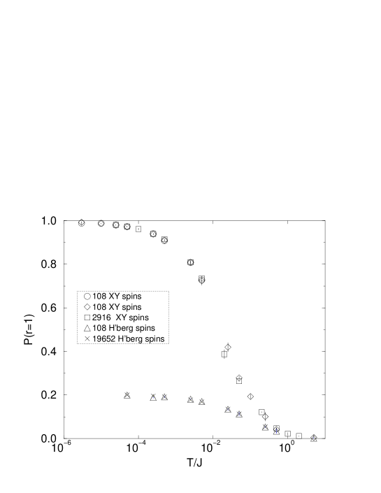
FIG. 11.: The temperature dependence of $P(r=1)$ for $XY$ and Heisenberg spins. Most error bars are smaller than the symbols. Simulations started from random initial spin configurations, except those for the data points marked with open circles, which started from collinear spin configurations.

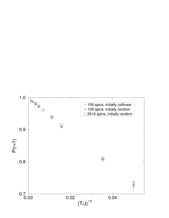
FIG. 12.: $P(r=1)$ versus $(T/J)^{1/2}$ for $XY$ spins.

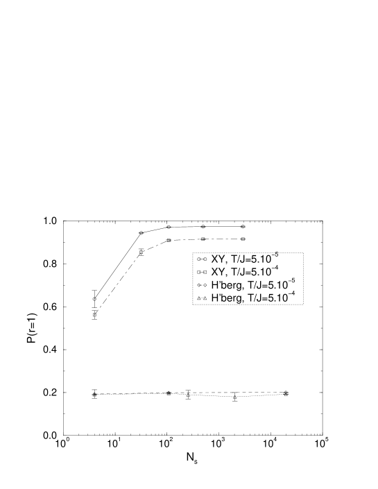
FIG. 13.: System size dependence of the collinearity parameter $P(r=1)$ for $XY$ and Heisenberg spins at $T=5\times 10^{-5}J$ and $T=5\times 10^{-4}J$.

B Specific heat

An unbiased way to search for soft fluctuations and – by implication – fluctuation-induced order is to measure heat capacity.[24] At low temperature, one expects to be able to describe fluctuations of the system from a ground state in terms of canonical coordinates which are almost independent of each other. From the classical equipartition theorem, a canonical coordinate, $p$, which appears in the Hamiltonian as $(p/p_{0})^{2r}$, contributes $k_{B}/(2r)$ to the heat capacity. Hence, each quadratic mode contributes $k_{B}/2$, and each quartic mode $k_{B}/4$, whereas zero modes do not contribute at all. Determining the heat capacity therefore allows a determination of the number of quadratic and quartic modes present.

If, as predicted, thermal fluctuations select a collinear state for the $XY$ model, then there is one quartic and one quadratic mode per tetrahedron. This results in a heat capacity per spin, $C$, of $3/8k_{B}$. In the absence of order, all modes are quadratic, and $C=k_{B}/2$. For the Heisenberg antiferromagnet, there are four degrees of freedom per tetrahedron, one of which is a zero mode. If there is no order, we expect $C=3/4k_{B}$; if a collinear state is selected by thermal fluctuations, $C=5/8k_{B}$. In finite-sized systems, the heat capacity per spin is reduced. For our choice of periodic boundary conditions, this manifests itself in the correction $C(N)=\left({(N-1)/{N}}\right)C(\infty)$.

As shown in Fig. 14, we find in the limit $N\rightarrow\infty$, that $C=0.376\pm 0.002$ for $XY$ spins, and that $C=0.747\pm 0.002$ for Heisenberg spins. This is consistent with the presence of order for $XY$ spins, with one quartic mode per tetrahedron, as expected. For Heisenberg spins, we obtain an upper limit of 0.04 quartic modes per tetrahedron.

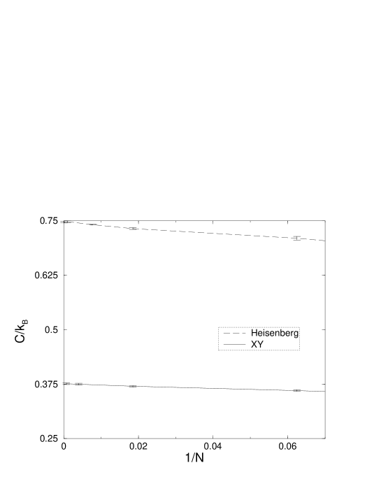
FIG. 14.: The specific heat for different system sizes for the $XY$ and the Heisenberg antiferromagnet on the pyrochlore lattice. The lines are a guide to the eye.

VI The dynamics of the pyrochlore antiferromagnet

We now turn to time-dependent correlation functions, and ask how the system explores the vicinity of its ground-state manifold at low temperature. We study the spin autocorrelation function with precessional dynamics, both analytically and by numerical integration of the equations of motion. Two of the facts established in the previous sections have important implications for spin dynamics. First, we have shown that the ground-state manifold is connected, which means that the magnet does not get trapped in a particular state at low temperatures by internal energy barriers. Second, we have shown that there is no entropic selection of special ground states at low temperatures, which suggests that the dynamics is unlikely to be hindered by free energy barriers. We indeed find that spin correlations relax relatively rapidly even at low temperatures, having a time-scale that diverges only as $T^{-1}$, and not, for example, according to an Arrhenius law.

A Derivation of an effective spin dynamics

Consider, in the first instance, the dynamics linearised around a ground state. In this approximation, a system of $N$ tetrahedra (hence with $2N$ spins and a $4N$-dimensional phase-space) will have $2N$ normal modes. Some of these modes will be conventional, finite frequency spin-waves, but a fraction will have zero frequency, because there is no restoring force for displacements in phase space that take the system from one ground state to another. Beyond the harmonic approximation, non-linear terms in the full equations of motion will have various consequences: the conventional, finite-frequency modes will acquire a finite lifetime; and coupling between these modes and the ground-state coordinates will drive the system around its ground-state manifold. We find that there are three distinct time-scales at low temperature. The period of the highest frequency spin-waves, $O(\hbar/J)$, sets the shortest scale; their lifetime, $\tau_{s}\sim\hbar/[Jk_{B}T]^{1/2}$, provides an intermediate scale; while the longest scale is the decay time of the autocorrelation function, $\tau\sim\hbar/k_{B}T$. This separation of time-scales greatly simplifies the problem.

Our starting point is the equation of motion,

$$\frac{d{\bf{S}}_{i}}{dt}={\bf{S}}_{i}\times{\bf H}_{i}(t)\equiv-J\,{\bf{S}}_{i}\times({\bf L}_{\alpha}+{\bf L}_{\beta}),$$ (6)

where we have set $\hbar=1$. ${\bf H}_{i}(t)$ is the exchange field acting at site $i$, which can be expressed in terms of ${\bf L}_{\alpha}$ and ${\bf L}_{\beta}$, the total spins of the two tetrahedra to which ${\bf{S}}_{i}$ belongs. Summing over the sites of a tetrahedron, the time-dependence of ${\bf L}_{\alpha}$ is

$$\frac{d{\bf L}_{\alpha}}{dt}=-J\,\sum_{\beta}{\bf{S}}_{\alpha\beta}\times{\bf L}_{\beta},$$ (7)

in which the notation ${\bf{S}}_{\alpha\beta}$ has been introduced for the spin common to the tetrahedra $\alpha$ and $\beta$.

The right side of Eq. 7 implicitly defines a $3N\times 3N$ matrix, ${\bf M}$, acting on a vector constructed from the components of the ${\bf L}_{\alpha}$’s. This matrix, being real and antisymmetric, has eigenvalues which are purely imaginary and occur in pairs, $\pm i\omega$, related by complex conjugation. For a ground-state spin configuration, the magnitudes of these eigenvalues are the frequencies of $3N/2$ normal modes, while the real and imaginary parts of the associated eigenvectors are canonically conjugate coordinates for the modes. The remaining $N$ directions in phase space are spanned by coordinates having ${\bf L}_{\alpha}=0$ for all $\alpha$, and therefore lie within the ground-state manifold. The matrix ${\bf M}$ is well-defined and has purely imaginary eigenvalues for any spin configuration; for a low-temperature spin configuration, the eigenvalue magnitudes are presumably good approximations to the normal mode frequencies in a nearby ground state. We display in Fig. 15 the density of states, $\rho(\omega)$, on a linear scale, obtained by diagonalising ${\bf M}$ for low-temperature pyrochlore spin configurations generated in a Monte Carlo simulation. It is noteworthy that $\rho(\omega)$ appears to be finite at $\omega=0$: $\rho(\omega)$ neither includes a divergent contribution, proportional to $\delta(\omega)$, nor does it vanish as $\omega\to 0$.

FIG. 15.: The density of states, $\rho(\omega)$ for a system of 2048 Heisenberg spins at low temperature.

The fact that $\rho(\omega)$ does not contain a delta function at $\omega=0$ gives information on how canonically conjugate pairs of coordinates appear in the linearised dynamics. Quite generally, the Hamiltonian in the harmonic approximation can be reduced to the form

$$H=\sum_{l=1}^{2N}(\alpha_{l}p_{l}^{2}+\beta_{l}q_{l}^{2}),$$ (8)

where $p_{l}$ and $q_{l}$ are a canonically conjugate pair of coordinates. We know from the ground-state construction described earlier that $1/4$ of these coordinates belong to the ground-state manifold, and therefore that $1/4$ of the $4N$ numbers $\{\alpha_{l},\beta_{l}\}$ are zero. Oscillations of the coordinates $p_{l},q_{l}$ have zero frequency if $\alpha_{l}\cdot\beta_{l}=0$, and so the fraction of zero-frequency spin-wave modes might, in principle, range from $1/4$, if for each of these modes both $\alpha_{l}=0$ and $\beta_{l}=0$, to $1/2$, if for each of these modes only one of $\alpha_{l}$ and $\beta_{l}$ is zero. The fact that $\rho(\omega)$ does not contain a delta function at $\omega=0$ implies that all (except for a fraction vanishing in the thermodynamic limit) of the $3N/2$ modes derived from ${\bf M}$ have non-zero frequency, and therefore that only the remaining $1/4$ of modes have zero frequency. Hence, for every $l$, either both $\alpha_{l}$ and $\beta_{l}$ are zero or neither is zero: coordinates in the ground-state manifold all appear in canonically conjugate pairs.

The non-zero density of states apparent at small frequency in Fig. 15 is in striking contrast to the behaviour, $\rho(\omega)\propto\omega^{2}$, that occurs in both Néel-ordered antiferromagnets (including ordered states of the pyrochlore antiferromagnet [48]) and conventional spin-glasses. The arguments used by Halperin and Saslow [60] and by Ginzburg [61] to predict propagating long-wavelength modes in spin-glasses depend on the ground state having a stiffness. This stiffness appears to be missing in ground states of the pyrochlore antiferromagnet, because of the many zero modes.

The exchange field, ${\bf H}_{i}(t)$, appearing in the equation of motion, Eq. 6, can be written as a superposition of contributions arising from the finite-frequency modes, in terms of vectors, ${\bf u}_{l}(i)$, determined by $\bf M$, and amplitudes, $A_{l}$, determined by the initial conditions:

$${\bf H}_{i}(t)=\sum_{l}A_{l}{\bf u}_{l}(i)e^{i\omega_{l}t}+c.c.\,.$$ (9)

In the harmonic approximation, the amplitudes, $A_{l}$, are time-independent, but in the full dynamics their magnitude and phase will change on a time-scale which defines the spin-wave lifetime, $\tau_{s}$. We postpone detailed discussion of the temperature dependence of $\tau_{s}$ until the end of this section, but note that, at low temperature, $\tau_{s}$ is large compared to the typical spinwave period, $J^{-1}$.

If the equation of motion is integrated over time-intervals longer than $\tau_{s}$, contributions from modes with frequencies $\omega_{l}\gg\tau_{s}^{-1}$ average to zero, while those from modes with $\omega_{l}\lesssim\tau_{s}^{-1}$ fluctuate randomly, according to the time-dependence of $A_{l}(t)$. Hence ${\bf H}_{i}(t)$ has mean value zero, and has fluctuations which are characterised most importantly by their low-frequency spectral density,

$$\int_{-\infty}^{\infty}dt^{\prime}\langle{\bf H}_{i}(t)\cdot{\bf H}_{i}(t^{\prime})\rangle\,\equiv\,2\Gamma\,.$$ (10)

In terms of the amplitudes, $A_{l}(t)$,

$$\Gamma=\sum_{l}\int\langle A_{l}(0)A_{l}^{*}(t)\rangle e^{i\omega_{l}t}|{\bf u}_{l}(i)|^{2}dt\,.$$ (11)

Since, for large $\tau_{s}$, only the low-frequency modes contribute to $\Gamma$, and since, from equipartition, $\langle|{\bf H}_{i}(t)|^{2}\rangle\sim J^{2}\langle|{\bf L}_{\alpha}|^{2}\rangle\sim Jk_{\rm B}T$, we have $\Gamma\propto Jk_{\rm B}T\rho(0^{+})$. Note that, as $\rho(\omega)\propto J^{-1}$, $\Gamma$ is independent of $J$.

We now proceed to calculate long-time spin correlations from Eq. 6, by treating ${\bf H}_{i}(t)$ as Gaussian white noise with the correlator

$$\langle{\bf H}_{i}(t)\cdot{\bf H}_{i}(t^{\prime})\rangle=2\Gamma\delta(t-t^{\prime})\,.$$ (12)

To do so involves several assumptions. The most important of these is that the spinwave lifetime, $\tau_{s}$, which sets the width in time of the delta function in Eq 12, is small compared to the decay time of the spin autocorrelation function. We show below that this is asymptotically exact as $T/J\to 0$. Further, in taking $\Gamma$ to be a constant, rather than a functional of the instantaneous spin configuration, we implicitly neglect variations with spin configuration in the local density of states, $\sum_{l}|{\bf u}_{l}(i)|^{2}\delta(\omega_{l})$. Such fluctuations certainly exist, but seem from our numerical studies only to have a small effect on the form of the spin autocorrelation function. Solving the Langevin equation that results from treating ${\bf H}_{i}(t)$ in Eq. 6 as white noise, we obtain $\langle{\bf{S}}_{i}(0)\cdot{\bf{S}}_{i}(t)\rangle=e^{-\Gamma t}$ and hence (reinstating $\hbar$)

$$\langle{\bf{S}}_{i}(0)\cdot{\bf{S}}_{i}(t)\rangle=\exp(-ck_{\rm B}Tt/\hbar)\,,$$ (13)

where $c$ is a dimensionless constant of order unity. Therefore, the autocorrelation time $\tau=\Gamma^{-1}=\hbar/(ck_{B}T)$. We emphasise again that, at $T\ll J/k_{\rm B}$, it is $T$ alone, and not $J$, which sets the scale for long-time dynamics.

To complete this discussion, it is necessary to estimate the spinwave lifetime, $\tau_{s}$. There are two physical processes that contribute to $\tau_{s}$. One, common to all antiferromagnets, is the anharmonic interaction between different finite-frequency modes, which here results in a lifetime varying as $T^{-1}$ for small $T$. It is, however, overwhelmed by a second process, specific to systems with many ground-state degrees of freedom, in which finite-frequency modes are mixed by the motion of the system between different ground states. More formally, on time scales $\gg\hbar/J$, the matrix ${\bf M}$ is time-dependent. The linearised equations of motion, with time-dependent ${\bf M}$, define an autonomous dynamical problem in which the instantaneous normal mode amplitudes, $A_{l}(t)$, are time-dependent. The time-dependence of the matrix elements of ${\bf M}$ mixes amplitude, initially concentrated in a single mode, $l$, over all modes lying within a window of frequencies around $\omega_{l}$. From time-dependent perturbation theory, a fractional change, $f$, in matrix elements spreads amplitude over a frequency window whose width, $\delta\omega$, forms a fraction $f$ of the entire spinwave spectrum, so that $\delta\omega\sim fJ/\hbar$. And from our results for the spin autocorrelation function, the fractional change in matrix elements during a time-interval $\tau_{s}$ is $f=k_{\rm B}T\tau_{s}/\hbar$. The spinwave lifetime is the time at which the frequency window resulting from this $f$ has width $\delta\omega\sim 1/\tau_{s}$, and so we obtain $\tau_{s}\sim\hbar/[Jk_{\rm B}T]^{1/2}$. As required for the consistency of our arguments, at low temperatures this is indeed a much shorter timescale than that for the decay of the spin autocorrelation function.

As the temperature is raised towards $T\sim J$, this separation of timescales breaks down. The precession on the previously shortest timescale then becomes visible, and the autocorrelation decays initially as $1-A(t)\propto t^{2}$ rather than $1-A(t)\propto t$. This is indeed observed in our numerical simulations described in the next section (Fig. 16).

B Molecular dynamics simulations

In this subsection, we present results obtained from numerical simulations of the dynamics of the Heisenberg pyrochlore antiferromagnet. In these simulations we evaluate the autocorrelation function

$$A(t)\equiv\left<{\bf{S}}_{i}(0)\cdot{\bf{S}}_{i}(t)\right>.$$ (14)

We find that $A(t)$ decays exponentially in time. The simulations confirm the predictions of the preceding section, namely that the timescale for the dynamics, $\tau$, varies as $T^{-1}$. Finally, we do not discover any sign of spin freezing even at temperatures as low as $T=5\times 10^{-4}J$.

We generate uncorrelated, thermalised initial configurations by Monte Carlo simulation, from which the equation of motion, Eq. 6, is integrated using a fourth-order Runge-Kutta algorithm. Related calculations for the kagome Heisenberg antiferromagnet have been described previously by Keren.[34]

Some details of our procedure are as follows. We choose the integration time-step so that energy is conserved to at least one part in $10^{8}$. The temperature range of the simulations covers three orders of magnitude, the lowest temperature being $T=5\times 10^{-4}J$. The system sizes studied range from 32 spins to 2048 spins. There are marked finite size effects in the smaller systems, which we believe result from all spins precessing together about the total magnetisation, ${\bf M}_{tot}$, of the system. Since $|{\bf M}_{tot}|^{2}\sim N$, the precession rate varies as $N^{-1/2}$, and decreases rather slowly with increasing system size. For the results presented, we hasten convergence to the thermodynamic limit by adding the term $J{\bf M}_{tot}^{2}$ to the Hamiltonian, which constrains the total magnetisation to be independent of system size and near zero. As a result, values of the decay time, $\tau$, coincide for systems with 500 and 2048 spins.

1 The functional form of $A(t)$

From the analytic calculation presented in subsection VI A, we expect $A(t)$ to depend on time and temperature only through the combined variable, $Tt$. We show in Fig. 16 $A(t)$ as a function of this scaling variable, at various temperatures and over one and a half decay times, $\tau$, for a system of 2048 spins. The collapse of the data onto a single curve, at all except the highest temperatures ($T/J\geq 0.1$), is striking evidence in support of our analytic results. To demonstrate the accuracy with which the decay of $A(t)$ at low temperature is exponential, and to indicate the magnitude of finite-size effects in our results, we show in Fig 17 data for $A(t)$ on a logarithmic scale, for runs starting from different initial configurations generated at the same temperature.

FIG. 16.: The autocorrelation function as a function of the rescaled time, $Tt$.

FIG. 17.: The decay of $A(t)$  on a logarithmic scale for five different runs at the same temperature, $T/J=6\times 10^{-3}$, in a system of 2048 spins.

To examine quantitatively the temperature dependence of the decay time, $\tau$, we fit data at each temperature to an exponential, $\exp\left(-t/\tau\right)$. The resulting values for $\tau$ are displayed in Fig. 18. In order to extract the temperature dependence of $\tau$, we fit it to the power law $\tau={\cal{A}}T^{-\zeta}$.[51] Excluding temperatures $T/J\geq 0.15$, we obtain $\zeta=0.998\pm 0.012$ and ${\cal{A}}=0.53\pm 0.04$. This result agrees with and confirms our prediction that $\zeta=1$.

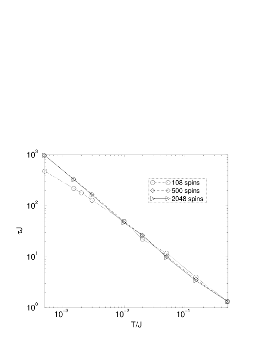
FIG. 18.: The decay time as a function of tempeature for three different system sizes.

C Inelastic neutron scattering

Inelastic neutron scattering provides the most detailed probe of dynamical correlations. We expect from the results described above that diffuse inelastic scattering in the temperature range $T_{F}<T\ll|\Theta_{CW}|$ should have a Lorentzian lineshape in energy, with a width, $\Gamma$, varying as $\Gamma=ck_{B}T$, where $c$ is of order unity. Although we have not explicitly examined the dependence of dynamic correlations on wavevector, $k$, it seems likely that main contribution to the inelastic linewidth in the low-temperature limit should be roughly wavevector independent. One reason for thinking this is that the decay of the autocorrelation function probably arises because of rotation of relatively small clusters of spins - the local ground-state degrees of freedom identified in III E. In consequence, we expect dynamical correlations to be short-ranged in space and broad in wavevector. In addition, conservation laws which might result in significantly different behaviour, for example $\Gamma\propto k^{2}$ for small $k$ from conservation of spin density, do not appear to be in operation: since the magnetisations of individual tetrahedra are identically zero in classical ground states, instantaneous magnetisation fluctuations can decay without spreading to large distances. Thermally induced fluctuations in the magnetisations of tetrahedra may result in an additional, diffusive component to spin correlations, with an amplitude that vanishes in the low-temperature limit.

Inelastic neutron scattering from the pyrochlore antiferromagnet $CsNiCrF_{6}$, which has $|\Theta_{CW}|\simeq 70$K and $T_{F}\simeq 2.2$K,[58] is reported in Ref. [16], in which the energy dependence of scattering is fitted by a Lorentzian. The linewidth decreases as temperature is decreased below 70 K, but the data seem insufficiently precise to test whether $\Gamma$ is linear in $T$. Similar experiments on $SCGO$, in which $|\Theta_{CW}|$ is around 500 K and $T_{F}\simeq 3.5$K, yield a Lorentzian inelastic lineshape with a temperature dependence of the width which is encouragingly close to linear, and of order $k_{B}T$, over the temperature range from $30K$ to $290K$.[7, 10]

VII Concluding remarks

We have presented a detailed theoretical analysis of the low-temperature properties of a class of geometrically frustrated classical antiferromagnets, with particular emphasis on the pyrochlore Heisenberg antiferromagnet, which has a macroscopically degenerate ground-state manifold. Given the connectedness of this ground-state manifold and the absence of appreciable free energy barriers, there seems to be no mechanism for localising the system in a particular region of the ground-state manifold, and it is therefore unlikely that the spin glass transition observed in most experiments is a feature of the disorder-free classical isotropic Heisenberg pyrochlore antiferromagnet. Rather, we find correlation functions to be short-ranged in both space and time, and conclude that the spins continue to fluctuate strongly down to the lowest temperatures.

We have analysed for the first time the low-energy dynamics of these geometrically frustrated antiferromagnets. Our discussion does not depend on details of the pyrochlore lattice structure. In fact, we expect it also to apply to the Heisenberg model defined on the $SCGO$-lattice of Fig. 3, since that model has $D_{M}/N>0$ and does not – following the arguments presented in Ref. [51] and Sect. IV – display order by disorder. These properties are in striking contrast to those of the kagome Heisenberg antiferromagnet, and $SCGO$ is much more similar to a pyrochlore magnet than to the kagome system.

We expect our results to be robust against the introduction of a small concentration of vacancies,[53] certainly provided the average defect spacing is larger than extent of the most local ground-state degree of freedom in the pure system. Behaviour characteristic of the pure system may persist to much higher defect concentrations, since $D_{M}/N>0$ as long as more than three quarters of all sites are occupied.

REFERENCES

- [1] For reviews, see: A. P. Ramirez, Annu. Rev. Mater. Sci. 24, 453, (1994); P. Schiffer and A. P. Ramirez, Comments Cond. Mat. Phys. 18, 21 (1996); and M. J. Harris and M. P. Zinkin, Mod. Phys. Lett. B 10, 417 (1996).
- [2] X. Obradors, A. Labarta, A. Isalgue, J. Tejada, J. Rodriguez and M. Pernet, Solid State Comm. 65, 189 (1988).
- [3] A. P. Ramirez, G. P. Espinosa and A. S. Cooper, Phys. Rev. Lett. 64, 2070 (1990).
- [4] C. Broholm, G. Aeppli, G. P. Espinosa and A. S. Cooper, Phys. Rev. Lett. 65, 3173 (1990).
- [5] A. P. Ramirez, G. P. Espinosa and A. S. Cooper, Phys. Rev. B 45, 2505 (1992).
- [6] B. Martinez, F. Sandiumenge, A. Rouco, A. Labarta, J. Rodriguezcarvajal, M. Tova, M. T. Causa, S. Gali and X. Obradors, Phys. Rev. B 46, 10786 (1992).
- [7] S.-H. Lee, C. Broholm, G. Aeppli, T. G. Perring, B. Hessen and A. Taylor, Phys. Rev. Lett. 76, 4424 (1996).
- [8] S.-H. Lee, C. Broholm, G. Aeppli, A. P. Ramirez, T. G. Perring, C. J. Carlile, M. Adams, T. J. L. Jones and B. Hessen, Europhys. Lett. 35, 127 (1996).
- [9] P. Schiffer, A. P. Ramirez, K. N. Franklin, and S.-W. Cheong, Phys. Rev. Lett. 77, 2085 (1996).
- [10] S.-H. Lee, Ph.D. thesis, Johns Hopkins University, 1996; S.-H. Lee, C. Broholm, G. Aeppli, T. G. Perring, B. Hessen, and A. Taylor, unpublished.
- [11] W. Kurtz and S. Roth, Physica 86-88B, 715 (1977).
- [12] L. Bevaart, P. M. H. L. Tegelaar, A. J. Van Duyneveldt and M. Steiner, Phys. Rev. B 26, 6150 (1982).
- [13] B. D. Gaulin, J. N. Reimers, T. E. Mason, J. E. Greedan and Z. Tun, Phys. Rev. Lett. 69, 3244 (1992).
- [14] J. E. Greedan, J. N. Reimers, C. V. Stager and S. L. Penny, Phys. Rev. B 43, 5682 (1991).
- [15] M. J. Harris, M. P. Zinkin, Z. Tun, B. M. Wanklyn, and I. P. Swanson, Phys. Rev. Lett. 73, 189 (1994).
- [16] M. J. Harris, M. P. Zinkin and T. Zeiske, Phys. Rev. B 52, R707 (1995).
- [17] M. P. Zinkin, M. J. Harris and T. Zeiske, Phys. Rev. B 56, 11786 (1997).
- [18] Y. J. Uemura, A. Keren, L. P. Le, G. M. Luke, B. J. Sternlieb and W. D. Wu, Hyperfine Interactions 85, 133 (1994).
- [19] S. R. Dunsiger, R. F. Kiefl, K. H. Chow, B. D. Gaulin, M. J. P. Gingras, J. E. Greedan, A. Keren, K. Kojima, G. M. Luke, W. A. Macfarlane, N. P. Raju, J. E. Sonier, Y. J. Uemura, W. D. Wu, Phys. Rev. B 54, 9019 (1996).
- [20] Y. J. Uemura, A. Keren, K. Kojima, L. P. Le, G. M. Luke, W. D. Wu, Y. Ajiro, T. Asano, Y. Kuriyama, M. Mekata, H. Kikuchi and K. Kakurai, Phys. Rev. Lett. 73, 3306 (1994).
- [21] N. P. Raju, E. Gmelin and R. K. Kremer, Phys. Rev. B 46, 5405 (1992).
- [22] J. N. Reimers, J. E. Greedan and M. Bjorgvinsson, Phys. Rev. B 45, 7295 (1992).
- [23] M. J. P. Gingras, C. V. Stager, N. P. Raju, B. D. Gaulin and J. E. Greedan, Phys. Rev. Lett. 78, 947 (1997) and references therein.
- [24] J. T. Chalker, P. C. W. Holdsworth and E. F. Shender, Phys. Rev. Lett. 68, 855 (1992).
- [25] I. Ritchey, P. Chandra and P. Coleman, Phys. Rev. B 47, 15342 (1993).
- [26] J. Villain, R. Bidaux, J. P. Carton and R. J. Conte, J. Phys. – Paris 41, 1263 (1980).
- [27] E. F. Shender, Zh. Eksp. Teor. Fiz. 83, 326 (1982) [Sov. Phys. JETP 56, 178 (1982)].
- [28] C. L. Henley, Phys. Rev. Lett. 62, 2056 (1989).
- [29] C. L. Henley, J. Appl. Phys. 61, 3962 (1987).
- [30] M. W. Long, J. Phys. C 2, 5383 (1990).
- [31] D. A. Huse and A. D. Rutenberg, Phys. Rev. B45, 7536 (1992).
- [32] P. Chandra and B. Doucot, J. Phys. A 27, 1541 (1994).
- [33] J. N. Reimers, Phys. Rev. B 45, 7287 (1992).
- [34] A. Keren, Phys. Rev. Lett. 72, 3254 (1994).
- [35] G. Ferey, R. De Pape, M. Leblanc and J. Pannetier, Rev. Chim. Miner. 23, 474 (1986).
- [36] J. N. Reimers, J. E. Greedan, C. V. Stager and M. Björgvinsson, Phys. Rev. B 43, 5692 (1991).
- [37] P. Chandra, P. Coleman and I. Ritchey, J. Phys. I France 3, 591 (1993).
- [38] M. J. Harris, S. T. Bramwell, D. F. McMorrow, T. Zeiske and K. W. Godfrey, Phys. Rev. Lett. 79, 2554 (1997).
- [39] R. Moessner, Phys. Rev. B 57, R5587 (1998).
- [40] E. F. Shender, V. B. Cherepanov, P. C. W. Holdsworth and A. J. Berlinsky, Phys. Rev. Lett. 70, 3812 (1993).
- [41] P. Schiffer, A. P. Ramirez, D. A. Huse, P. L. Gammel, U. Yaron, D. J. Bishop and A. J. Valentino, Phys. Rev. Lett. 74, 2379 (1995).
- [42] J. N. Reimers, A. J. Berlinsky and A.-C. Shi, Phys. Rev. B 43, 865 (1991).
- [43] A. B. Harris, C. Kallin and A. J. Berlinsky, Phys. Rev. B 45, 2899 (1992).
- [44] A. B. Harris, A. J. Berlinsky and C. Bruder, J. Appl. Phys. 69, 5200 (1991).
- [45] J. B. Marston and C. Zeng, J. Appl. Phys. 69, 5962 (1991).
- [46] S. Sachdev, Phys. Rev. B 45, 12377 (1992).
- [47] A. Chubukov, Phys. Rev. Lett. 69, 832 (1992).
- [48] R. R. Sobral and C. Lacroix, Solid State Comm. 103, 407 (1997).
- [49] P. Lecheminant, B. Bernu, C. Lhuillier, L. Pierre and P. Sindzingre, Phys. Rev. B 56, 2521 (1997). and references therein.
- [50] B. Canals and C. Lacroix, Phys. Rev. Lett. 80, 2933 (1998).
- [51] R. Moessner and J. T. Chalker, Phys. Rev. Lett. 80, 2929 (1998).
- [52] R. Moessner, D.Phil. thesis, University of Oxford, 1997.
- [53] J. Villain, Z. Phys. B 33, 31 (1979).
- [54] S. T. Bramwell, M. J. P. Gingras and J. N. Reimers, J. Appl. Phys. 75, 5523 (1994).
- [55] J. C. Maxwell, Phil. Mag. 27, 294 (1864).
- [56] R. Liebmann, Statistical Mechanics of Periodic Frustrated Ising Systems (Springer, Berlin, 1986).
- [57] P. W. Anderson, Phys. Rev. 102, 1008 (1956).
- [58] M. P. Zinkin, D.Phil. thesis, University of Oxford, 1996.
- [59] E. F. Shender, and P. C. W. Holdsworth, Order by disorder and topology in frustrated magnetic systems in M. M. Millonas (ed.) Fluctuations and Order: The New Synthesis (MIT Press, Boston, 1994).
- [60] B. I. Halperin and W. M. Saslow, Phys. Rev. B 16, 2154 (1977).
- [61] S. L. Ginzburg, Zh. Eksp. Teor. Fiz. 75, 1497 (1978). [Sov. Phys. JETP 48, 756 (1978).]