The half-filled Hubbard chain in the Composite Operator Method: A comparison with Bethe Ansatz

Abstract

The one-dimensional Hubbard model at half-filling is studied in the framework of the Composite Operator Method using a static approximation. A solution characterized by strong antiferromagnetic correlations and a gap for any nonzero on-site interaction $U$ is found. The corresponding ground-state energy, double occupancy and specific heat are in excellent agreement with those obtained within the Bethe Ansatz. These results show that the Composite Operator Method is an appropriate framework for the half-filled Hubbard chain and can be applied to evaluate properties, like the correlation functions, which cannot be obtained by means of the Bethe Ansatz, except for some limiting cases.

1 Introduction

New materials whose physics is dominated by electron correlations in narrow energy bands are actually a challenge for solid state physicists. The treatment of such systems is not trivial due to the competition between itinerant and localized behaviour of the electrons in these bands. The Hubbard Hamiltonian [1] is regarded as the simplest model which can give us the basic understanding of the effects of strong electronic correlations. In particular, its one-dimensional (1D) version is interesting for several reasons. On the one hand it is exactly integrable, by means of the Bethe Ansatz [2]. On the other, it could be applied to study real quasi-1D systems like the $KCP$ and $TTF-TCNQ$ salts [3], the doped spin Peierls chains [4] and the Cu-O chains of the high-$T_{c}$ superconductors, whose underlying physics is directly related to the low-dimensionality of the system.

By using the Bethe Ansatz and following a method developed by Yang [5], Lieb and Wu evaluated exactly some ground-state properties of the 1D Hubbard model at half filling [6]. Two years later, the spin and charge excitation spectra were obtained, also within the Bethe Ansatz, by Ovchinnikov [7]. For arbitrary electron density, the Bethe Ansatz coupled integral equations for the charge and spin distribution functions cannot be analytically solved except in some limiting cases [8] and numerical calculation is needed. In this way, Shiba [9] evaluated the ground state energy, local magnetic moment and magnetic susceptibility as a function of the electron density. The finite-temperature formalism of the Bethe Ansatz developed by Takahashi [10] provides the evaluation of the thermodynamic properties [11]. Further studies of the 1D Hubbard model within the framework of the Bethe Ansatz have clarified for instance the thermodynamics in the presence of a magnetic field [12].

Therefore, we see that the Bethe Ansatz allows to exactly evaluate many quantities, thus providing a wide picture of the physics of the Hubbard chain. Nevertheless, this Ansatz cannot be regarded as a complete framework since many important properties, like the charge and spin correlation functions and the spectral properties, cannot be extracted from the exact Bethe Ansatz wave function except for some limiting cases (e.g. half filling, $U\rightarrow\infty$, $\omega=0$) [13]. Otherwise we must address to other numerical [14] or analytical [15] approaches.

The Bethe Ansatz is a very useful test for any approximation scheme, whose reliability can be checked by computing quantities that are given exactly by such Ansatz. In this sense, many of the available analytical methods do not give satisfactory results. On the other hand, all numerical techniques present some inherent problems, namely the small size of the clusters and the impossibility of reaching very low temperatures. Motivated by this, we have studied the 1D Hubbard model at half filling by means of an analytic approach that has proved to be adequate for studying other strongly correlated models [16]. The results obtained for the thermodynamic properties are in good agreement with the numerical data [17], also some anomalous thermodynamic and magnetic behaviours observed in high-$T_{c}$ cuprate superconductors have been successfully explained [17, 18]. In this calculation scheme, called the Composite Operator Method (COM), the long-lived excitations of the system are described by an appropriate combination of the standard fermionic field operators. The properties of the new fermionic fields are self-consistently determined by the dynamics. To fix the internal parameters that appear, some symmetry requirements, like the Pauli principle and the particle-hole symmetry, are imposed. This procedure permits to recover symmetries that are badly violated by other approaches [19], and thus is expected to provide a better description of strongly correlated systems [20].

In this letter we analyze the half-filled infinite Hubbard chain within COM in the static approximation, where finite life-time effects are neglected. Although we are considering a paramagnetic (PM) ground state, we find a solution of the model which shows strong antiferromagnetic (AF) features. We present a detailed analysis of this AF-like solution. We calculate the energy and double occupancy of the ground-state, and the specific heat as a function of temperature, and compare them to the exact results obtained by the Bethe Ansatz. Excellent agreement is found.

2 Method

We consider the well-known Hubbard Hamiltonian:

$$H=\sum_{ij}t_{ij}c^{\dagger}\left(i\right)c\left(j\right)+U\sum_{i}n_{\uparrow}\left(i\right)n_{\downarrow}\left(i\right)-\mu\sum_{i}n(i)$$ (1)

where $c^{\dagger}\left(i\right)=\left(c_{\uparrow}^{\dagger}\left(i\right),c_{\downarrow}^{\dagger}\left(i\right)\right)$ is the electron operator on the site $i$ in the spinor notation, $n_{\sigma}\left(i\right)$ is the charge–density operator for the spin $\sigma$, $\mu$ is the chemical potential introduced to control the particle density $n=\langle c^{\dagger}(i)c(i)\rangle$, and $U$ is the on-site Coulomb interaction. Considering only nearest neighbours and taking the lattice constant as one, the hopping matrix for the chain is

$$t_{ij}=-2t\frac{1}{N}\sum_{k}e^{ik\left(i-j\right)}cos(k)$$ (2)

In the case of the Hubbard model, a natural choice for the composite operators is the Hubbard doublet $\Psi^{\dagger}=(\xi^{\dagger}(i),\eta^{\dagger}(i))$, where

$$\xi^{\dagger}(i) = c^{\dagger}(i)\,[1-n(i)]$$

$$\eta^{\dagger}(i) = c^{\dagger}(i)\,n(i)$$ (3)

This operators describe the hopping of an electron to an unoccupied and to an occupied site $i$, respectively. Considering a two-pole approximation [21] and a PM ground state, the Fourier transform of the single-particle retarded thermal Green’s function may be written in COM as:

$$S\left(k,\omega\right)=\sum_{i=1}^{2}\frac{\sigma^{(i)}\left(k\right)}{\omega-E_{i}\left(k\right)}$$ (4)

The energy bands are given by $E_{i}(k)=R(k)+(-)^{i+1}\,Q(k)$ where

$$R(k) = \frac{U}{2}-\mu-2t\,cos(k)-\frac{m(k)}{2\,I_{1}I_{2}}$$

$$Q(k) = \frac{1}{2}\sqrt{\left(U-\frac{m(k)}{I_{1}I_{2}}\right)^{2}+2nU\,\frac{m(k)}{I_{1}I_{2}}}$$ (5)

$$m(k) = 2t[\Delta+\cos(k)\,(p-I_{2})]$$

and $I_{1}$, $I_{2}$ are the diagonal matrix elements of the normalization matrix $I=F.T.\left\langle\left\{\Psi(i),\Psi^{\dagger}(j)\right\}\right\rangle$. The spectral moments $\sigma^{(i)}(k)$ that appear in the Green’s function (4) are given in ref. [16, 21].

As shown above, the single-particle thermal Green’s function (4) depends on the external parameters $t$, $U$, $n$ and $T$ (temperature), and three internal parameters $\mu$, $\Delta$ and $p$. $\Delta$ and $p$ are the following intersite charge correlation function and intersite charge, spin and pair correlation function, respectively [16, 20].

$$\Delta = \langle\xi^{\alpha}(i)\xi^{\dagger}(i)\rangle-\langle\eta^{\alpha}(i)\eta^{\dagger}(i)\rangle$$

$$p = \frac{1}{4}\langle n_{\mu}^{\alpha}(i)n_{\mu}(i)\rangle-\langle(c_{\uparrow}(i)c_{\downarrow}(i))^{\alpha}\,c_{\downarrow}^{\dagger}(i)c_{\uparrow}^{\dagger}(i)\rangle$$ (6)

The superscript $\alpha$ indicates the field on the first neighbour sites and $n_{\mu}(i)=c^{\dagger}(i)\sigma_{\mu}c(i)$ is the charge- ($\mu=0$) and spin- ($\mu=1,2,3$) density operator, where $\sigma_{\mu}$ is the Pauli representation of the $SU(2)$ symmetry group. These parameters roughly produce (see eq. (5)) a shift in the bands ($\Delta$) and a bandwidth renormalization ($p$). Very different results are obtained according to how these internal parameters are fixed [20]. In COM they are determined by solving the following system of coupled self-consistent equations,

$$\left\{\begin{array}[]{l}n=2\left(1-S_{11}-S_{22}\right)\\ \Delta=S_{11}^{\alpha}-S_{22}^{\alpha}\\ S_{12}=0\end{array}\right.$$ (7)

with $S_{\gamma\delta}=\left\langle\Psi_{\gamma}(i)\Psi^{\dagger}_{\delta}(i)\right\rangle$ and $S_{\gamma\delta}^{\alpha}=\left\langle\Psi^{\alpha}_{\gamma}(i)\Psi^{\dagger}_{\delta}(i)\right\rangle$.

The first two equations are obtained from the existing relations with the elements of the Green’s function, and the third one comes from requiring the satisfaction of the Pauli principle at the level of matrix elements (see ref. [16, 20] for details).

Once the internal parameters are determined, the evaluation of the physical quantities is straightforward. In this paper we study the single-particle band structure, the energy and double occupancy of the ground state, and the specific heat. The band structure is determined from eq. (5)). The ground-state energy per site is calculated as the thermal average of the Hamiltonian and is given by

$$E=2t\left(G_{1}-(1-n)UF_{1}+\frac{B_{1}}{I_{1}I_{2}}\right)+\frac{I_{2}}{2}U(1-G_{0}-UF_{0})$$ (8)

where the functions $F_{n}$, $G_{n}$ and $B_{n}$ ($n=0,1,\cdots$) are defined in ref. [20].

We use the thermodynamic relations $E=F+TS$,

$$F(T,n)=\int_{0}^{n}\,\mu(T,n^{\prime})\,dn^{\prime}\hskip 28.45274ptS(T,n)=-\int_{0}^{n}\,\left(\frac{\partial\mu}{\partial T}\right)_{n^{\prime}}\,dn^{\prime}$$ (9)

with $F$ the Helmholtz free energy and $S$ the entropy, to determine the specific heat, which reads as

$$C(T,n)=-T\int_{0}^{n}\,\left(\frac{\partial^{2}\mu}{\partial T^{2}}\right)_{n^{\prime}}\,dn^{\prime}$$ (10)

As shown for the 2D case [17], the temperature derivatives of the chemical potential can be expressed in terms of the internal parameters and calculated once the self-consistent equations (7) are solved. Finally, the double occupancy is calculated by deriving the free energy with respect to $U$.

3 Results

Considering a PM ground state, we find a fully self-consistent solution characterized by a negative value of the $p$ parameter. The results for the energy spectrum are shown in fig. 1. As we can see, this solution presents a typical AF band pattern; namely, a first excitation at $k=\pm\frac{\pi}{2}$, a very narrow bandwidth of order $J=\frac{2t^{2}}{U}$ (the AF exchange interaction), and a quasi-halved Brillouin zone. Such an AF-like band structure is directly related to the negative sign of the $p$ parameter, which is responsible of the general band shape [see eq. (5)]. In the figure, the energy is measured with respect to the chemical potential. The solution exhibits a gap in the excitation spectrum for any non-zero value of $U$, in agreement with the Bethe Ansatz solution. The rate at which the gap increases coincides with Bethe Ansatz down to $U\approx 4$.

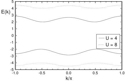
Fig. 1.–: Band structure of the half-filled Hubbard chain at $T=0$ for the indicated couplings.

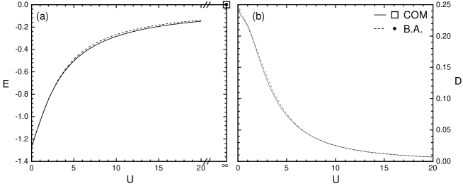
Fig. 2.–: $(a)$ Ground-state energy and $(b)$ double occupancy of the half-filled Hubbard chain in COM (solid line) and Bethe’s Ansatz (dashed line).

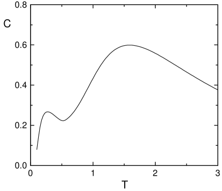
Fig. 3.–: Specific heat versus temperature of the half-filled Hubbard chain in COM for $U=8$.

We calculate the ground-state energy and double occupancy as indicated in the previous section. These quantities, as a function of $U$, are shown in fig. 2 together with Bethe’s Ansatz. The excellent agreement obtained is probably related to the opening of the gap mentioned above. Such a good agreement with Bethe Ansatz is not reached by other analytical approaches like the Gutzwiller approximations or the ladder and self-consistent ladder approximation [15]. In particular, these approaches fail to reproduce the correct asymptotic behaviour of the ground-state energy. As shown in panel $(b)$, the double occupancy goes to zero as $U\rightarrow\infty$. In a system of itinerant electrons with an average of one electron per site, the kinetic energy must also have this asymptotic behaviour, because any electron hopping would lead to a double occupied site. Therefore, electrons localize at infinite $U$, where the half-filled Hubbard chain is equivalent to the spin-$\frac{1}{2}$ AF Heisenberg chain that describes a system of localized spins.

We calculate the specific heat of the system by means of eq. (10). The result as a function of temperature and for a ratio $\frac{U}{W}=2$ (coupling/bandwidth) is shown in fig. 3. A double-peak structure appears, with a first peak located at $T\approx 0.25$ and a second one at $T\approx 1.6$ ($T$ is measured in units of $t$). This is in good agreement with the Bethe Ansatz calculation of Ref. [11]. The low-$T$ feature is due to the spin excitations, since $0.25$ is precisely the magnitude of the AF exchange parameter $J=\frac{2t^{2}}{U}$ for $U=8$ and a peak at such location is also found in the AF Heisenberg chain [22]. The high-$T$ peak is associated to charge excitations. We can reach this interpretation by examining the chemical potential as a function of the electron density for several temperatures. At very low $T$, $\mu$ has a discontinuity at $n=1$ of magnitude $U$ that leads to the opening of a gap in the charge excitation spectrum, as we commented above. For increasing $T$ the discontinuity in $\mu$ is smoothed because the electrons can be excited across the gap. Therefore, charge excitations appear in the system at higher temperatures. Such a specific heat structure of the 1D Hubbard model, with low- and high- $T$ regions dominated by spin and charge excitations, respectively, is also obtained by numerical calculations on finite chains [23]. In the weak-intermediate-coupling regime $\left(\frac{U}{W}\leq 1\right)$ charge and spin excitations cannot be distinguished since they are of the same energy range, and hence the specific heat shows only one peak [23].

4 Conclusions

Summarizing, we have studied the 1D Hubbard model at half filling by means of the COM considering a PM state and a two-pole approximation. Within this approach we find a solution of the model that reproduces very well the exact solution given by the Bethe Ansatz. Namely, we obtain an insulating ground state characterized by strong AF correlations for any non-zero interaction $U$. The energy and double occupancy of this AF-like ground state is in excellent agreement with that of Bethe Ansatz. We have also calculated the temperature dependence of the specific heat of the system in the strong coupling regime. The locations of the spin- and charge-excitation peaks are consistent with the ones of the Bethe Ansatz. The approximation considered seems thus to be an adequate framework to study the physics of the half-filled Hubbard chain. It is of particular interest to apply this approach to get information about properties, like the correlation and spectral functions, which cannot be extracted from the Bethe Ansatz, except for some limits.

The good agreement obtained for the ground-state energy and double occupancy within a static approximation is not surprising. As it is well known, such an approach gives a good description of the high-energy sector even though is unable to distinguish the low-energy features. Anyway, these features, are swallowed when integrating over the whole energy range. In this line of thinking, it is worth noticing the good description that we obtain for both the low- and high- energy sector of the specific heat. We suspect that this is due to our correct treatment of the Pauli principle at the level of matrix elements. In a physics dominated by strong electronic correlations, we believe that the satisfaction of the Pauli principle not only at the operator level, but also at the level of observation (relation among matrix elements) is crucial.

***

The authors wish to thank F. D. Buzatu for many valuable discussions. M. M. Sánchez acknowledges a grant from the Instituto Nazionale per la Fisica della Materia (INFM).

References

- [1] J. Hubbard, Proc. Roy. Soc. London A, 276 (1963) 238.
- [2] H. Bethe, Z. Physik, 71 (1931) 205.
- [3] D. Jérome and A. J. Schulz, Adv. Phys., 31 (1982) 299; C. S. Jacobsen, I. Johannsen and K. Bechgaard, Phys. Rev. Lett., 53 (1984) 194.
- [4] T. M. Rice, in Physics in One Dimension, edited by J. Bernasconi and T. Schneider, Vol. 23 (Springer Series in Solid-State Sciences) 1981, pp. 229-238.
- [5] C. N. Yang, Phys. Rev. Lett., 19 (1967) 1312.
- [6] E. H. Lieb and F. Y. Wu, Phys. Rev. Lett., 20 (1968) 1445.
- [7] A. A. Ovchinnikov, Sov. Phys. JETP, 30 (1970) 1160.
- [8] J. Carmelo and D. Baeriswyl, Phys. Rev. B, 37 (1988) 7541.
- [9] H. Shiba, Phys. Rev. B, 6 (1972) 930.
- [10] M. Takahashi, Prog. Theor. Phys., 47 (1972) 69.
- [11] N. Kawakami, T. Usuki and A. Okiji, Phys. Lett. A, 137 (1989) 287; T. Usuki, N. Kawakami and A. Okiji, Journ. Phys. Society of Japan, 59 (1990) 1357.
- [12] J. Carmelo, P. Horsch, P. A. Bares and A. A. Ovchinnikov, Phys. Rev. B, 44 (1991) 9967.
- [13] M. Ogata and H. Shiba, Phys. Rev. B, 41 (1990) 2326; N. Kawakami and A. Okiji, Phys. Rev. B, 40 (1989) 7066; N. Kawakami and S.-K. Yang, Phys. Rev. Lett., 65 (1990) 3063; H. J. Schulz, Phys. Rev. Lett., 64 (1990) 2831; S. Sorella and A. Parola, J. Phys. Condens. Matter, 4 (1992) 3589; B.S. Shastry and B. Sutherland, Phys. Rev. Lett., 65 (1990) 243.
- [14] S. Sorella et al., Europhys. Lett., 12 (1990) 721; J. H. Xu and J. Yu, Phys. Rev. B, 45 (1992) 6931 ; R. Preuss et al., Phys. Rev. Lett., 73 (1994) 732.
- [15] W. Metzner and D. Vollhardt, Phys. Rev. Lett., 59 (1987) 121; F. D. Buzatu, Mod. Phys. Lett. B, 9 (1995) 1149; J. E. Hirsch, Phys. Rev. B, 22 (1980) 5259.
- [16] S. Ishihara et al., Phys. Rev. B, 49 (1994) 1350; F. Mancini et al., Physica C, 244 (1995) 49; 250 (1995) 184; 252 (1995) 361; F. Mancini et al., Phys. Lett. A, 210 (1996) 429; A. Avella et al., Physica C, 282–287 (1997) 1757; 282–287 (1997) 1759.
- [17] F. Mancini, D. Villani and H. Matsumoto, cond-mat/9709189.
- [18] F. Mancini et al., Phys. Rev. B, 57 (1998) 6145; A. Avella et al., Phys. Lett. A, 240 (1998) 235.
- [19] D. J. Rowe, Rev. Mod. Phys., 40 (1968) 153.
- [20] A. Avella et al., Int. J. Mod. Phys. B, 12 (1998) 81.
- [21] F. Mancini, cond-mat/9803276.
- [22] J. Bonner and M. Fisher, Phys. Rev., 135 (1964) A640.
- [23] H. Shiba and P. A. Pincus, Phys. Rev. B, 5 (1972) 1966; J. Schulte and M. Böhm, Phys. Rev. B, 53 (1996) 15385.