Fermi liquids and Luttinger liquids

1 Introduction

In these lecture notes, corresponding roughly to lectures given at the summer school in Chia Laguna, Italy, in September 1997, an attempt is made to present the physics of three–dimensional interacting fermion systems (very roughly) and that of their one–dimensional counterparts, the so–called Luttinger liquids (in some more detail). These subjects play a crucial role in a number of currently highly active areas of research: high temperature and organic superconductors, quantum phase transitions, correlated fermion systems, quantum wires, the quantum Hall effect, low–dimensional magnetism, and probably some others. Some understanding of this physics thus certainly should be useful in a variety of areas, and it is hoped that these notes will be helpful in this.

As the subject of these lectures was quite similar to those delivered at Les Houches, some overlap in the notes[1] was unavoidable. However, a number of improvements have been made, for example a discussion of the “Klein factors” occurring in the bosonization of one–dimensional fermions, and new material added, mainly concerning spin chains and coupled Luttinger liquids. Some attempt has been made to keep references up to date, but this certainly has not always been successful, so we apologize in advance for any omissions (but then, these are lecture notes, not a review article).

2 Fermi Liquids

Landau’s Fermi liquid theory[2, 3, 4] is concerned with the properties of a many–fermion system at low temperatures (much lower than the Fermi energy) in the normal state, i.e. in the absence or at least at temperatures above any symmetry breaking phase transition (superconducting, magnetic, or otherwise). The ideal example for Landau’s theory is liquid helium 3, above its superfluid phase transition, however, the conceptual basis of Landau’s theory is equally applicable to a variety of other systems, in particular electrons in metals. Quantitative applications are however more difficult because of a variety of complications which appear in real systems, in particular the absence of translational and rotational invariance and the presence of electron–phonon interactions, which are not directly taken into account in Landau’s theory. Subsequently, I will first briefly discuss the case of a noninteracting many–fermion system (the Fermi gas), and then turn to Landau’s theory of the interacting case (the liquid), first from a phenomenological point of view, and then microscopically. A much more detailed and complete exposition of these subjects can be found in the literature [5, 6, 7, 8, 9].

2.1 The Fermi Gas

In a noninteracting translationally invariant systems, the single-particle eigenstates are plane waves

$$|{{\mathbf{k}}}\rangle=\frac{1}{\sqrt{\Omega}}{e}^{{\rm i}{{\mathbf{k}}}\cdot{\mathbf{r}}}$$ (2.1)

with energy

$$\varepsilon_{{{\mathbf{k}}}}=\frac{{{\mathbf{k}}}^{2}}{2m}\;\;,$$ (2.2)

where $\Omega$ is the volume of the system, and we will always use units so that $\hbar=1$. The ground state of an $N$–particle system is the well–known Fermi sea: all states up to the Fermi wavevector ${k_{\rm F}}$ are filled, all the other states are empty. For spin–1/2 fermions the relation between particle number and ${k_{\rm F}}$ is

$$N=\Omega\frac{{k_{\rm F}}^{3}}{3\pi^{2}}\;\;.$$ (2.3)

The energy of the last occupied state is the so–called Fermi energy $E_{\rm F}={k_{\rm F}}^{2}/(2m)$, and one easily verifies that

$$E_{\rm F}=\frac{\partial E_{0}(N)}{\partial N}=\mu(T=0)$$ (2.4)

i.e. $E_{\rm F}$ is the zero–temperature limit of the chemical potential ($E_{0}(N)$ in the formula above is the ground state energy).

It is usually convenient to define the Hamiltonian in a way so that the absolute ground state has a well–defined fixed particle number. This is achieved simply by including the chemical potential $\mu$ in the definition of the Hamiltonian, i.e. by writing

$$H=\sum_{{{\mathbf{k}}}}\xi_{{{\mathbf{k}}}}n_{{{\mathbf{k}}}}\;\;,$$ (2.5)

where $n_{{\mathbf{k}}}$ is the usual number operator, $\xi_{{\mathbf{k}}}=\varepsilon_{{\mathbf{k}}}-\mu$, and the spin summation is not written explicitly (at finite temperature this of course brings one to the usual grand canonical description where small fluctuations of the particle number occur). With this definition of the Hamiltonian, the elementary excitations of the Fermi gas are

• addition of a particle at wavevector ${{\mathbf{k}}}$ ($\delta n_{{\mathbf{k}}}=1$). This requires $|{{\mathbf{k}}}|>{k_{\rm F}}$, and thus the energy of this excitation is $\varepsilon_{{\mathbf{k}}}=\epsilon_{{\mathbf{k}}}-\mu>0$.

• destruction of a particle at wavevector ${{\mathbf{k}}}$ ($\delta n_{{\mathbf{k}}}=-1$), i.e. creation of a hole. This requires $|k|<{k_{\rm F}}$, and thus the energy is $\varepsilon_{k}=\mu-\epsilon_{{\mathbf{k}}}>0$.

The dispersion relation of the elementary particle and hole excitation is shown in fig.1a.

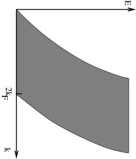
Figure 1: (a) the energy–momentum relation for the elementary particle ($k>{k_{\rm F}}$) and hole ($k<{k_{\rm F}}$) excitations; and (b) the particle–hole continuum.

These excitations change the total number of particles. Construction of states at constant particle number is of course straightforward: one takes one particle from some state ${{\mathbf{k}}}$, with $|k|<{k_{\rm F}}$, and puts it into a state ${{\mathbf{k}}}^{\prime}$, with $|{{\mathbf{k}}}^{\prime}|>{k_{\rm F}}$. These particle–hole excitations are parameterized by the two quantum numbers ${{\mathbf{k}}}$,${{\mathbf{k}}}^{\prime}$ and thus form a continuum, as shown in fig.1b. The restriction on the allowed values of ${{\mathbf{k}}},{{\mathbf{k}}}^{\prime}$ insures that all particle–hole states have positive energy. Higher excited states, i.e. states with many particles and many holes, are straightforwardly constructed, the only restriction being imposed by the Pauli principle.

Thermodynamic quantities are easily obtained and are all determined by the density of states at the Fermi energy. For example, the specific heat obeys the well known linear law $C(T)=\gamma T$, with

$$\gamma=\frac{2\pi^{2}}{3}N(E_{\rm F})k_{\rm B}^{2}$$ (2.6)

and similarly the (Pauli) spin susceptibility $\chi$ and the compressibility $\kappa$ are given by

$$\chi = 2N(E_{\rm F})\mu_{\rm B}^{2}$$ (2.7)

$$\kappa = 2N(E_{\rm F})/\rho^{2}\;\;.$$ (2.8)

Here for the quadratic dispersion relation (2.2) the density of states (per spin) at the Fermi energy is given by $N(E_{\rm F})=m{k_{\rm F}}/(2\pi^{2})$, but it should be emphasized that eqs. (2.6) to (2.8) are valid for an arbitrary density of states, in particular in solids where bandstructure effects can change the electronic dispersion relation quite drastically. Thus, for noninteracting electrons one expects the so–called “Wilson ratio”

$$R_{W}=\frac{\pi^{2}k_{\rm B}^{2}}{3\mu_{\rm B}^{2}}\frac{\chi}{\gamma}$$ (2.9)

to be unity, independently of details of the bandstructure. Any deviation from unity is necessarily an indication of some form of interaction effect.

2.2 Landau’s theory of Fermi Liquids

2.2.1 Basic hypothesis

Landau’s theory is to a large extent based on the idea of a continuous and one–to–one correspondence between the eigenstates (ground state and excited states) of the noninteracting and the interacting system. For this to be an acceptable hypothesis it is crucial that the interactions do not lead to any form of phase transition or symmetry–broken ground state.

In particular one can consider a state obtained by adding a particle (with momentum $|{\mathbf{p}}|>{k_{\rm F}}$) to the noninteracting ground state:

$$|{\mathbf{p}},N+1\rangle=a_{{\mathbf{p}}}^{+}|0,N\rangle\;\;.$$ (2.10)

Here $a_{{\mathbf{p}}}^{+}$ is a fermion creation operator for momentum state ${\mathbf{p}}$, and $|0,N\rangle$ is the $N$–particle ground state of the noninteracting system. Now we add some form of particle–particle interaction. In a translationally invariant system, interactions conserve total momentum, and thus even after switching on the interaction the state still has total momentum ${\mathbf{p}}$. However, the interaction of the added particle with the filled Fermi sea, as well as the interaction of the particles in the sea amongst themselves, will change the distribution of particles in ${{\mathbf{k}}}$–space, and of course also modify the energy of our state. The complex formed by the particle added at ${\mathbf{p}}$ and the perturbed distribution of the other particles is called a Landau quasiparticle. The Pauli principle implied $|{\mathbf{p}}|>{k_{\rm F}}$ in the absence of interactions, and by the continuity hypothesis the same restriction remains valid in the interacting case. In particular, the value of ${k_{\rm F}}$, which imposes a lower limit on the allowed momentum of the quasiparticle, is unchanged by the interactions.

Analogous considerations can be performed for a state obtained by destruction of a particle (e.g. creation of a hole):

$$|{\mathbf{p}},N-1\rangle=a_{{\mathbf{-}p}}|0,N\rangle\;\;.$$ (2.11)

Note that due to the momentum $-{\mathbf{p}}$ the total momentum of this state is indeed ${\mathbf{p}}$.

The quasi–particle concept has a certain number of limitations, mainly due to the fact that, as will be discussed below, the lifetime of a quasi–particle is finite. However, for excitations close to ${k_{\rm F}}$ one has $1/\tau\propto(\varepsilon-E_{\rm F})^{2}$, i.e. the lifetime becomes much longer than the inverse excitation energy, and the quasi–particles therefore are reasonably well defined. In practice, this means that Landau’s theory is useful for phenomena at energy scales much smaller than the Fermi energy, but inapplicable otherwise. In metals, where $E_{\rm F}\approx 3\ldots 5eV$, this restriction is not too serious when one is concerned with thermodynamic or transport properties. One should also note that the ground state energy itself has important contributions from states well below $E_{\rm F}$, and therefore is not accessible to Landau’s theory.

2.2.2 Equilibrium properties

In order to derive physical quantities from the picture of the low–energy excitations, we need some information about the energetics of the quasiparticles and of their interactions. To be specific, starting from the ground state quasiparticle distribution

$$n_{0}({{\mathbf{k}}}) = 1\;\mbox{if $|{{\mathbf{k}}}|<{k_{\rm F}}$}$$ (2.12)

$$= 0\;\mbox{if $|{{\mathbf{k}}}|>{k_{\rm F}}$}$$

one considers changes in quasiparticle occupation number of the the form $n_{0}(k)\rightarrow n_{0}(k)+\delta n(k)$, i.e. $\delta n(k)=1$ represents an excited quasi–particle, $\delta n(k)=-1$ an excited quasi–hole (with the notation $k=({{\mathbf{k}}},\sigma)$, and $\sigma=\uparrow,\downarrow$ the spin index). The corresponding change in energy is

$$\delta E=\sum_{k}\varepsilon_{{\mathbf{k}}}^{0}\delta n(k)+\frac{1}{2\Omega}\sum_{kk^{\prime}}f(k,k^{\prime})\delta n(k)\delta n(k^{\prime})\;\;,$$ (2.13)

where the first and second term represent the energy of a single quasi–particle and the interaction between quasiparticles, respectively. To be more precise, we assume that the chemical potential is included in the Hamiltonian, as in eq.(2.5). Consequently, $\varepsilon^{0}_{{\mathbf{k}}}$ vanishes on the Fermi surface, and, given that we are mainly interested in phenomena in the vicinity of ${k_{\rm F}}$, it is sufficient to retain the lowest order term in an expansion around $|{{\mathbf{k}}}|={k_{\rm F}}$. One thus writes

$$\varepsilon_{{\mathbf{k}}}^{0}=\frac{{k_{\rm F}}}{m^{*}}(|{{\mathbf{k}}}|-{k_{\rm F}})\;\;,$$ (2.14)

thus defining the effective mass $m^{*}$ which is different from the “bare” mass $m$ due to interaction effects that could in principle be calculated from a microscopic theory of the system.

The energy of a quasi–particle added to the system is easily obtained from eq.(2.13) by calculating the difference in $\delta E$ between a state with $\delta n(k)=1$ and a state with $\delta n(k)=0$. One finds

$$\varepsilon_{k}=\varepsilon^{0}_{{\mathbf{k}}}+\frac{1}{\Omega}\sum_{k^{\prime}}f(k,k^{\prime})\delta n(k^{\prime})\;\;,$$ (2.15)

i.e. the energy of an added quasi–particle is not just the “bare” quasiparticle energy $\varepsilon^{0}_{{\mathbf{k}}}$ but also depends, via the interaction term, on the presence of the other quasi–particles. Given that the non–interacting particles obey Fermi–Dirac statistics, the quasi–particles do so too, and consequently, the occupation probability of a quasi–particle state is given by

$$n(k)=\frac{1}{{e}^{\beta\varepsilon_{k}}+1}\;\;.$$ (2.16)

Note that the full and not the bare quasi–particle energy enters this expression. In principle, $n(k)$ thus has to be determined self-consistently from eqs.(2.15) and (2.16).

For the subsequent calculations, it is convenient to transform the quasiparticle interaction $f(k,k^{\prime})$. First, spin symmetric and antisymmetric $f$–functions are defined via

$$f({{\mathbf{k}}}\uparrow,{\mathbf{k}^{\prime}}\uparrow) = f^{s}({{\mathbf{k}}},{{\mathbf{k}}}^{\prime})+f^{a}({{\mathbf{k}}},{{\mathbf{k}}}^{\prime})$$

$$f({{\mathbf{k}}}\uparrow,{\mathbf{k}^{\prime}}\downarrow) = f^{s}({{\mathbf{k}}},{{\mathbf{k}}}^{\prime})-f^{a}({{\mathbf{k}}},{{\mathbf{k}}}^{\prime})$$ (2.17)

Moreover, given the implicit restrictions of the theory, one is only interested in processes where all involved particles are very close to the Fermi surface. Under the assumption that the interaction functions are slowly varying as a function of ${{\mathbf{k}}}$, one then can set $|{{\mathbf{k}}}|=|{{\mathbf{k}}}^{\prime}|={k_{\rm F}}$. Because of rotational symmetry, the $f$–functions then can only depend on the angle between ${{\mathbf{k}}}$ and ${{\mathbf{k}}}^{\prime}$, called $\theta$. One can then expand the $f$–function in a Legendre series as

$$f^{a,s}({{\mathbf{k}}},{{\mathbf{k}}}^{\prime})=\sum_{L=0}^{\infty}f_{L}^{a,s}P_{L}(\cos\theta)\;\;,\cos\theta=\frac{{{\mathbf{k}}}\cdot{{\mathbf{k}}}^{\prime}}{{k_{\rm F}}^{2}}\;\;,$$ (2.18)

where the $P_{L}$ are the Legendre polynomials. Finally, one usually puts these coefficients into dimensionless form by introducing

$$F_{L}^{a,s}=\frac{{k_{\rm F}}m^{*}}{\pi^{2}}f_{L}^{a,s}\;\;.$$ (2.19)

We are now in a position to calculate some equilibrium properties. The first one will be the specific heat at constant volume

$$C_{\Omega}=\frac{1}{\Omega}\frac{\partial U}{\partial T}$$ (2.20)

where $U$ is the internal energy. The temperature–dependent part of $U$ comes from thermally excited quasi–particles, as determined by the distribution (2.16). In principle, in this expression $\varepsilon_{k}$ is itself temperature–dependent, because of the temperature dependent second term in eq.(2.15). However, one can easily see that this term only gives contributions of order $T^{2}$, and therefore can be neglected in the low–temperature limit. Consequently, one can indeed replace $\varepsilon_{k}$ by $\varepsilon^{0}_{{\mathbf{k}}}$, and then one only has to replace the bare mass by $m^{*}$ in the result for a non–interacting system to obtain

$$C_{\Omega}=\frac{m^{*}{k_{\rm F}}}{3}k_{\rm B}^{2}T\;\;.$$ (2.21)

The spin susceptibility (at $T=0$) is related to the second derivative of the ground state energy with respect to the (spin) magnetization $M$:

$$\chi=\left[\Omega\frac{\partial^{2}E_{0}}{\partial M^{2}}\right]^{-1}\;\;.$$ (2.22)

Spin magnetization is created by increasing the number of $\uparrow$ spin particles and decreasing the number of $\downarrow$ spins ($M=\mu_{\rm B}(N_{\uparrow}-N_{\downarrow})$), i.e. by changing the Fermi wavevectors for up and down spins: ${k_{\rm F}}\rightarrow{k_{\rm F}}+\delta{k_{\rm F}}$ for $\sigma=\uparrow$ and ${k_{\rm F}}\rightarrow{k_{\rm F}}-\delta{k_{\rm F}}$ for $\sigma=\downarrow$.

By calculating with eq.(2.13) the corresponding change of the ground state energy, we obtain from eq.(2.22):

$$\chi=\frac{1}{1+F_{0}^{a}}\frac{\mu_{\rm B}^{2}{k_{\rm F}}m^{*}}{\pi^{2}}\;\;,$$ (2.23)

Note that here, and contrary to the specific heat, interactions enter not only via $m^{*}$ but also explicitly via the coefficient $F_{0}^{a}$, which is the only coefficient that appears here because the distortion of the Fermi distribution function is antisymmetric in the spin index and has spherical symmetry ($L=0$). The Wilson ratio is then

$$R_{W}=\frac{1}{1+F_{0}^{a}}\;\;.$$ (2.24)

Following a similar reasoning, one can calculate the compressibility $\kappa$ of a Fermi liquid:

$$\kappa=-\frac{1}{\Omega}\frac{\partial\Omega}{\partial P}=\left[\Omega\frac{\partial^{2}E_{0}}{\partial\Omega^{2}}\right]^{-1}=\frac{m^{*}{k_{\rm F}}}{\pi^{2}\rho^{2}(1+F^{s}_{0})}\;\;.$$ (2.25)

It is also interesting that in a translationally invariant system as we have considered here, the effective mass is not independent of the interaction coefficients. One can show indeed, by exploiting the Galilean invariance of the system, that

$$\frac{m^{*}}{m}=1+F_{1}^{s}/3\;\;.$$ (2.26)

2.2.3 Nonequilibrium properties

As far as equilibrium properties are concerned, Landau’s theory is phenomenological and makes some important qualitative predictions, the most prominent being that even in the presence of interactions the low–temperature specific heat remains linear in temperature and that the spin susceptibility tends to a constant as $T\rightarrow 0$. However, Landau’s theory has little quantitative predictive power because the crucial Landau parameters have actually to be determined from experiment. The situation is different for non–equilibrium situations, where the existence of new phenomena, in particular collective modes, is predicted. These modes are another kind of elementary excitations which, contrary to quasiparticles, involve a coherent motion of the whole system. We shall not enter into the details of the treatment of non–equilibrium properties of Fermi liquids (see refs.[5, 8, 9]) and just briefly sketch the general conceptual framework and some of the more important results. To describe non–equilibrium situations, one makes two basic assumptions:

• Deviations from equilibrium are described by a Boltzmann equation for a space– and time– dependent quasiparticle distribution function $n({{\mathbf{k}}},{{\mathbf{r}}},t)$, which describes the density of quasi–particles of momentum and spin $({{\mathbf{k}}},\sigma)$ at point ${{\mathbf{r}}}$ and time $t$. At equilibrium, $n$ is of course given by eq.(2.12). The fact that in the distribution function one specifies simultaneously momentum and position of course imposes certain restrictions, due to the quantum–mechanical nature of the underlying problem. More precisely, spatial and temporal variations of the distribution function have to be slow compared to the typical wavelength and frequency of the quasiparticles. We have then the conditions $v_{\rm F}|{{\mathbf{q}}}|,|\omega|<E_{\rm F}$, where ${{\mathbf{q}}}$ and $|\omega|$ set the scale of the spatial and temporal variations of $n({{\mathbf{r}}},t)$.

• Because of the ${{\mathbf{r}}}$–dependent $n$, the quasiparticle energy is itself, via eq.(2.15), ${{\mathbf{r}}}$–dependent. One then assumes the following quasi–classical equations of motion

  $$\dot{{{\mathbf{r}}}} = {\mathbf{\nabla}}_{{\mathbf{k}}}\varepsilon_{{\mathbf{k}}}({{\mathbf{r}}})$$

  $$\dot{{{\mathbf{k}}}} = -{\mathbf{\nabla}}_{{\mathbf{r}}}\varepsilon_{{\mathbf{k}}}({{\mathbf{r}}})\;\;.$$ (2.27)

  Note in particular that a space–dependent distribution function gives rise, via the $f(k,k^{\prime})$ function, to a force acting on a quasiparticle.

By linearizing the Boltzmann equation and studying the collisionless regime, where the collision term in the Boltzmann equation can be neglected, one finds collective mode solutions which correspond to oscillations of the Fermi surface. The most important one is the longitudinal symmetric mode which, like ordinary sound, involves fluctuations of the particle density. This kind of sound appears, however, in a regime where ordinary sound cannot exist (the existence of collisions is indeed crucial for the propagation of ordinary sound waves) and is a purely quantum effect. Since collisions can always be neglected at very low temperatures, this new kind of sound has been called by Landau zero sound. The collision term of the Boltzmann equation is on the contrary essential to calculate the quasiparticle lifetime $\tau$. One can find indeed, for a quasiparticle of energy $\varepsilon_{{\mathbf{p}}}$

$$\tau^{-1}\propto m^{*3}\frac{(\pi T)^{2}+\varepsilon_{{\mathbf{p}}}^{2}}{1+\\ e^{-\beta\varepsilon_{{\mathbf{p}}}}}\;\;.$$ (2.28)

The most important result here is the divergence of the lifetime for low energies and temperatures as $\tau\propto\max(\varepsilon_{{\mathbf{p}}},T)^{-2}$, so that the product $\varepsilon_{{\mathbf{p}}}\tau$ in fact diverges as the Fermi surface is approached. This shows that the quasiparticle becomes a well–defined (nearly–) eigenstate at low excitation energies, i.e. in the region where Landau’s theory is applicable. On the other hand, at higher energies the quasiparticle becomes less and less well–defined. One may note that initially we had assumed that a quasiparticle is an exact eigenstate of the interacting system, which was obtained from a noninteracting eigenstate by switching on the interaction, and therefore should have infinite lifetime. We now arrive at the conclusion that the lifetime is not strictly infinite, but only very long at low energies. In the following section we will try to clarify this from a microscopical point of view.

2.3 Microscopic basis of Landau’s theory

At our current knowledge, it does not seem generally possible to derive Landau’s theory starting from some microscopic Hamiltonian, apart possibly in perturbation theory for small interactions. It is however possible to formulate the basic hypotheses in terms of microscopic quantities, in particular one– and two–particle Green functions. This will be outlined below.

2.3.1 Quasiparticles

As far as single particle properties are concerned it is sufficient to consider the one–particle Green function

$${\cal G}(k,\tau)=-\langle T_{\tau}a_{k}(\tau)a^{+}_{k}(0)\rangle\;\;,$$ (2.29)

where $\tau$ is the usual (Matsubara) imaginary time. In this quantity, interaction effects appear via self–energy corrections $\Sigma$ in the Fourier transformed function

$${\cal G}(k,\omega)=\frac{1}{{\rm i}\omega-\varepsilon_{k}^{00}-\Sigma(k,\omega)}\;\;.$$ (2.30)

Here $\varepsilon_{k}^{00}$ is the bare particle energy, without any effective mass effects. Excitation energies of the system then are given by the poles of ${\cal G}(k,\omega)$. In these terms, Landau’s assumption about the existence of quasiparticles is equivalent to assuming that $\Sigma(k,\omega)$ is sufficiently regular close to the Fermi surface as to allow an expansion for small parameters. Regularity in $({{\mathbf{k}}},\omega)$ space implies that in real space the self–energy has no contributions that decay slowly in time and/or space. Given that the self–energy can be calculated in terms of the effective interaction between particles this is certainly a reasonable assumption when the particle–particle interaction is short–range (though there is no formal prove of this). For Coulomb interactions, screening has to be invoked to make the effective interaction short ranged.

Figure 2: The momentum distribution function $n_{{\mathbf{k}}}=\langle a^{+}_{{\mathbf{k}}}a_{{\mathbf{k}}}\rangle$ in the interacting (full line) and noninteracting (dashed line) cases.

One can further notice that $\Sigma({k_{\rm F}},0)$ just renormalizes the chemical potential. Given that we want to work at fixed particle number we can absorb this term in the effective $\mu$. Expanding then to first order around the Fermi surface, the Green function takes the form

$${\cal G}(k,\omega)=\frac{z}{{\rm i}\omega-\varepsilon_{{\mathbf{k}}}^{0}}\;\;.$$ (2.31)

where $\varepsilon_{{\mathbf{k}}}^{0}$ has the form (2.14) of the phenomenological approach, with

$$m^{*}=m\left(1-\frac{\partial\Sigma}{\partial\omega}\right)\left(1+\frac{m}{{k_{\rm F}}}\frac{\partial\Sigma}{\partial k}\right)^{-1}\;\;,$$ (2.32)

and the quasiparticle renormalization factor is

$$z=\left(1-\frac{\partial\Sigma}{\partial\omega}\right)^{-1}\;\;.$$ (2.33)

All derivatives are to be taken at the Fermi surface and at $\omega=0$. One should notice that a sum rule imposes that the frequency–integrated spectral density

$$A(k,\omega)=-\frac{1}{\pi}{\rm Im}\,{\cal G}(k,i\omega\rightarrow\omega+i\delta)$$ (2.34)

equals unity. Consequently, in order to fulfill the sum rule, if $z<1$ there has to be a contribution in addition to the quasiparticle pole in eq.(2.31). This is the so–called “incoherent background” from single and multiple particle–hole pair excitations which can extend to rather high energies but becomes small close to the Fermi surface.

The form (2.31) gives rise to a jump in the momentum distribution function at ${k_{\rm F}}$ of height $z$, instead of unity in the noninteracting case (fig.2). In addition to the jump, the incoherent background gives rise to a contribution which is continuous through ${k_{\rm F}}$.

A finite quasiparticle lifetime arises if the expansion of $\Sigma(k,\omega)$ is carried to second order. Then eq.(2.31) generalizes to

$${\cal G}(k,\omega)=\frac{z}{{\rm i}\omega-\varepsilon_{{\mathbf{k}}}^{0}+{\rm i}{\rm sign}(\omega)\tau(\omega)^{-1}}\;\;,$$ (2.35)

where $\tau(\omega)$ is typically given by an expression like eq.(2.28).

2.3.2 Quasiparticle interaction

The quasiparticle interaction parameters $f(k,k^{\prime})$ are expected to be connected to the the two–particle vertex function. This function, which we will denote $\Gamma^{(2)}(P_{1},P_{2};K)$ describes the scattering of two particles from initial state $P_{1},P_{2}$ to the final state $P_{1}-K,P_{2}+K$, and the notation is $P_{i}=({{\mathbf{p}}}_{i},\omega_{i},\sigma_{i})$. The contribution of first and second order in the interaction potential $V({{\mathbf{k}}})$ are shown in fig.3.

         

Figure 3: The lowest (a) and second order (b) contributions to the two–particle vertex $\Gamma^{(2)}$. Note that the external lines do not represent actual Green functions but only indicate the external “connections”

Let us now study the case of small transfer $K$, but arbitrary $P_{1,2}$, only restricted to be close to the Fermi surface. One then notices that diagram 3b (part c) gives rise to singularities, because the poles of the two intervening Green functions coalesce. On the other hand diagrams 3b (part a) and 3b (part b) remain nonsingular for small $K$. This motivates one to introduce a two–particle irreducible function $\tilde{\Gamma}^{(2)}$ which is the sum of all contributions which do not contain a single product ${\cal G}(Q){\cal G}(K+Q)$. This function then is nonsingular for small $K$, and consequently the total vertex function is determined by the integral equation

$$\Gamma(P_{1},P_{2};K)=\tilde{\Gamma}(P_{1},P_{2})+\frac{1}{(2\pi)^{4}}\int{d}\omega{d}^{3}q\tilde{\Gamma}(P_{1},Q){\cal G}(Q){\cal G}(K+Q)\Gamma(Q,P_{2},K)\;\;.$$ (2.36)

For simplicity, the spin summation is omitted here. The singular contribution now comes from small $K$ and $Q$ in the vicinity of the Fermi surface. In this area the $Q$–dependence of the $\Gamma$’s in eq.(2.36) is non–singular and can be neglected. The energy and radial momentum integral over $Q$ can then be done, leading to

$$\Gamma(P_{1},P_{2};K)=\tilde{\Gamma}(P_{1},P_{2})+\frac{z^{2}{k_{\rm F}}^{2}}{(2\pi)^{3}}\int{d}^{2}\Omega_{{\mathbf{q}}}\tilde{\Gamma}(P_{1},Q)\frac{\hat{{{\mathbf{q}}}}\cdot{{\mathbf{k}}}}{\omega-v_{\rm F}\hat{{{\mathbf{q}}}}\cdot{{\mathbf{k}}}}\Gamma(Q,P_{2},K)\;\;,$$ (2.37)

where $\hat{{{\mathbf{q}}}}$ is a vector on the Fermi surface, and ${d}^{2}\Omega_{{\mathbf{q}}}$ is the corresponding angular integration. Here only the quasiparticle pole in ${\cal G}$ has been taken into account. The contribution from the incoherent parts can in principle be absorbed into the definition of $\tilde{\Gamma}$.

The expression (2.37) is clearly singular because it has radically different behavior according to whether one first sends ${{\mathbf{k}}}$ or $\omega$ to zero. In the first case, the limit of $\Gamma$ can be related to the Landau $f$–function, while the second one is relevant for the calculation of the transition probabilities determining the lifetime of quasiparticles. Here we will consider only the former case. Sending ${{\mathbf{k}}}$ to zero first one finds straightforwardly

$$\lim_{\omega\rightarrow 0}(\lim_{{{\mathbf{k}}}\rightarrow 0}\Gamma)\equiv\Gamma^{\omega}(P_{1},P_{2})=\tilde{\Gamma}(P_{1},P_{2})\;\;.$$ (2.38)

Closer inspection then shows that in this case the poles of the two Green functions in eq.(2.36) are always on the same side of the real axis and consequently the singular term in eq.(2.36) vanishes. To make the identification between $\Gamma^{\omega}(P_{1},P_{2})$ and the Landau $f$–function we notice that the density response function at energy–momentum $K$, whose poles give the collective (zero–sound) modes, contains the interactions via $\Gamma(P_{1},P_{2},K)$. In particular, the existence of a pole in the response function implies a pole in $\Gamma$. The comparison between the equations for this pole and those which can be obtained through the Boltzmann equation within Landau’s theory allows then the identification

$$f(k,k^{\prime})=z^{2}\Gamma^{\omega}(k,k^{\prime})\;\;.$$ (2.39)

2.4 Summary

The basic assumption of Landau’s theory is the existence of low–energy quasiparticles with a very long lifetime, and their description in terms of a rather simple energy functional, eq.(2.13). From this a number of results for thermodynamic properties is obtained. At this level, the theory is of little quantitative power because the Landau parameters are not determined. Qualitatively, however, the predictions are important: the low–temperature thermodynamic properties of an interacting fermion system are very similar to those of a noninteracting system, the interactions only lead to quantitative renormalizations. Actual quantitative predictions are obtained when one extends the theory to nonequilibrium properties, using the Boltzmann equation.[5] A new phenomenon predicted (and actually observed in $\rm{}^{3}He$ [10]) is the existence of collective excitations, called “zero sound”. This approach also allows the calculation of the quasiparticle lifetime and its divergence as the Fermi energy is approached, as well as the treatment of a number of transport phenomena.

As already mentioned, the ideal system for the application of Landau’s theory is $\rm{}^{3}He$, which has both short–range interaction and is isotropic. The application to electrons in metals is more problematic. First, the interactions are long–ranged (Coulombic). This can however be accommodated by properly including screening effects. More difficulties, at least at the quantitative level, arise because metals are naturally anisotropic. This problem is not of fundamental nature: even when the Fermi surface is highly anisotropic, an expansion like eq.(2.13) can still be written down and thus interaction parameters can be defined. However, a simple Legendre expansion like eq.(2.18) is not in general possible and the description of the quasiparticle interaction in terms of a few parameters becomes impossible. An exception case, with a very nearly spherical Fermi surface, are the alkali metals, where a determination of Landau parameters can indeed be attempted.[5] It should be noticed that the difficulties with the Landau description of metals are not of conceptual nature and in particular do not invalidate the quasiparticle concept but are rather limitations on the usefulness of the theory for quantitative purposes.

Landau’s theory can be interpreted in terms of microscopic quantities like Green functions (the quasiparticle pole) and interaction vertices, as discussed above. It should however be emphasized that these arguments do provide a microscopic interpretation of Landau’s picture, rather than proving its correctness. Similar remarks apply to the calculated diverging quasiparticle lifetime: this at best show that Landau’s picture is internally consistent. Considerable progress towards a deeper formal understanding of Fermi liquid theory has been made in recent years.[11, 12]

3 Renormalization group for interacting fermions

In this chapter, we will consider properties of interacting fermions in the framework of renormalization group theory. This will serve two purposes: first, the treatment of one–dimensional interacting fermions, which will be considered in considerable detail in the following chapters, gives rise to divergences which can only be handled by this approach. Results obtained in this way will be an essential ingredient in the subsequent discussion of “Luttinger liquids”. More generally, the renormalization group method will clarify the status of both Landau’s Fermi liquid theory and the Luttinger liquid picture as renormalization group fixed points, thus establishing a link with a number of other phenomena in condensed matter physics. We will formulate the problem in terms of fermion functional integrals, as done by Bourbonnais in the one–dimensional case [13] and more recently for two and three dimensions by Shankar [14]. For the most part, I will closely follow Shankar’s notation.

Before considering the interacting fermion problem in detail, let us briefly recall the general idea behind the renormalization group, as formulated by Kadanoff and Wilson: one is interested in the statistical mechanics of a system described by some Hamiltonian $H$. Equilibrium properties then are determined by the partition function

$$Z=\sum_{\mbox{configurations}}{e}^{-\beta H}=\sum_{\mbox{configurations}}{e}^{-S}\;\;,$$ (3.1)

where the second equality defines the action $S=\beta H$. Typically, the action contains degrees of freedom at wavevectors up to some cutoff $\Lambda$, which is of the order of the dimensions of the Brillouin zone. One wishes to obtain an “effective action” containing only the physically most interesting degrees of freedom. In standard phase transition problems this is the vicinity of the point ${{\mathbf{k}}}=0$, however, for the fermion problem at hand the surface $|{{\mathbf{k}}}|={k_{\rm F}}$ is relevant, and the cutoff has to be defined with respect to this surface. In order to achieve this one proceeds as follows:

1. Starting from a cutoff–dependent action $S(\Lambda)$ one eliminates all degrees of freedom between $\Lambda$ and $\Lambda/s$, where $s$ is a factor larger than unity. This gives rise to a new action $S^{\prime}(\Lambda^{\prime}=\Lambda/s)$.

2. One performs a “scale change” ${{\mathbf{k}}}\rightarrow s{{\mathbf{k}}}$. This brings the cutoff back to its original value and a new action $S^{\prime}(\Lambda)$ is obtained. Because of the degrees of freedom integrated out, coupling constants (or functions) are changed.

3. One chooses a value of $s$ infinitesimally close to unity: $s=1+\varepsilon$, and performs the first two steps iteratively. This then gives rise to differential equations for the couplings, which (in favorable circumstances) can be integrated until all non–interesting degrees of freedom have been eliminated.

3.1 One dimension

The one–dimensional case, which has interesting physical applications, will here be mainly used to clarify the procedure. Let us first consider a noninteracting problem, e.g. a one–dimensional tight–binding model defined by

$$H=\sum_{k}\xi_{k}a^{\dagger}_{k}a^{\phantom{\dagger}}_{k}\;\;,\quad\xi_{k}=-2t\cos k-\mu\;\;,$$ (3.2)

where $t$ is the nearest–neighbor hopping integral. We will consider the metallic case, i.e. the chemical potential is somewhere in the middle of the band. Concentrating on low–energy properties, only states close to the “Fermi points” $\pm{k_{\rm F}}$ are important, and one can then linearize the dispersion relation to obtain

$$H=\sum_{k,r=\pm}v_{F}(rk-{k_{\rm F}})a^{\dagger}_{kr}a^{\phantom{\dagger}}_{kr}\;\;,$$ (3.3)

where $v_{F}=2t\sin{k_{\rm F}}$ is the Fermi velocity, and the index $r$ differentiates between right– and left–going particles, i.e. particles close to ${k_{\rm F}}$ and $-{k_{\rm F}}$. To simplify subsequent notation, we (i) choose energy units so that $v_{F}=1$, (ii) translate $k$-space so that zero energy is at $k=0$, and (iii) replace the $k$–sum by an integral. Then

$$H=\sum_{r=\pm}\int_{-\Lambda}^{\Lambda}\frac{{d}k}{2\pi}rka^{\dagger}_{r}(k)a^{\phantom{\dagger}}_{r}(k)\;\;.$$ (3.4)

For the subsequent renormalization group treatment we have to use a functional integral formulation of the problem in terms of Grassmann variables (a detailed explanation of this formalism is given by Negele and Orland [15]). The partition function becomes

$$Z(\Lambda)=\int{\cal D}\phi{e}^{-S(\Lambda)}\;\;,$$ (3.5)

where ${\cal D}\phi$ indicates functional integration over a set of Grassmann variables. The action is

$$S(\Lambda)=\int_{0}^{\beta}{d}\tau\left\{\sum_{r=\pm}\int_{-\Lambda}^{\Lambda}\frac{{d}k}{2\pi}\phi_{r}^{*}(k,\tau)\partial_{\tau}\phi^{\phantom{*}}_{r}(k,\tau)+H(\phi^{*},\phi)\right\}\;\;,$$ (3.6)

where the zero–temperature limit $\beta\rightarrow\infty$ has to be taken, and $H(\phi^{*},\phi)$ indicates the Hamiltonian, with each $a^{\dagger}$ replaced by a $\phi^{*}$, and each $a$ replaced by a $\phi$. Fourier transforming with respect to the imaginary time variable

$$\phi_{r}(k,\tau)=T\sum_{\omega_{n}}\phi_{r}(k,\omega_{n}){e}^{-{\rm i}\omega_{n}\tau}\quad(\omega_{n}=2\pi(n+1/2)T)$$ (3.7)

and passing to the limit $T\rightarrow 0$ one obtains the noninteracting action

$$S_{0}(\Lambda)=\sum_{r=\pm}\int_{-\infty}^{\infty}\frac{{d}\omega}{2\pi}\int_{-\Lambda}^{\Lambda}\frac{{d}k}{2\pi}\phi_{r}^{*}(k,\omega)[-{\rm i}\omega+rk]\phi^{\phantom{*}}_{r}(k,\omega)\;\;.$$ (3.8)

We notice that this is diagonal in $k$ and $\omega$ which will greatly simplify the subsequent treatment. Because of the units chosen, $\omega$ has units of (length)^-1 (which we will abbreviate as $L^{-1}$), and then $\phi_{r}(k,\omega)$ has units $L^{3/2}$.

We now integrate out degrees of freedom. More precisely, we will integrate over the strip $\Lambda/s<|k|<\Lambda$, $-\infty<\omega<\infty$. The integration over all $\omega$ keeps the action local in time. One then has

$$Z(\Lambda)=Z(\Lambda,\Lambda/s)Z(\Lambda/s)\;\;,$$ (3.9)

where $Z(\Lambda,\Lambda/s)$ contains the contributions from the integrated degrees of freedom, and $Z(\Lambda/s)$ has the same form of eq.(3.5). The new action is then $S^{\prime}_{0}(\Lambda/s)=S_{0}(\Lambda/s)$. Introducing the scale change

$$k^{\prime}=ks\;\;,\quad\omega^{\prime}=\omega s\;\;,\quad\phi^{\prime}=\phi s^{-3/2}$$ (3.10)

one easily finds that $S^{\prime}_{0}(\Lambda)=S_{0}(\Lambda)$. The action does not change therefore under scale change (or renormalization): we are at a fixed point. One should notice that the scale change of $k$ implies that $k^{\prime}$ is quantized in in units of $\Delta k^{\prime}=2\pi s/L$, i.e. eliminating degrees of freedom actually implies that we are considering a shorter system, with correspondingly less degrees of freedom. This means that even though the action is unchanged the new $Z(\Lambda)$ is the partition function of a shorter system. To derive this in detail, one has to take into account the change in the functional integration measure due to the scale change on $\phi$.

Before turning to the problem of interactions, it is instructive to consider a quadratic but diagonal perturbation of the form

$$\delta S_{2}=\sum_{r=\pm}\int_{-\infty}^{\infty}\frac{{d}\omega}{2\pi}\int_{-\Lambda}^{\Lambda}\frac{{d}k}{2\pi}\mu(k,\omega)\phi_{r}^{*}(k,\omega)\phi^{\phantom{*}}_{r}(k,\omega)\;\;.$$ (3.11)

We assume that $\mu(k,\omega)$ can be expanded in a power series

$$\mu(k,\omega)=\mu_{00}+\mu_{10}k+\mu_{01}{\rm i}\omega+\ldots$$ (3.12)

Under the scale change (3.10) one then has

$$\mu_{nm}\rightarrow s^{1-n-m}\mu_{nm}\;\;.$$ (3.13)

There now are three cases:

1. a parameter $\mu_{nm}$ grows with increasing $s$. Such a parameter is called relevant. This is the case for $\mu_{00}$.

2. a parameter remains unchanged ($\mu_{10}$,$\mu_{01}$). Such a parameter is marginal.

3. Finally, all other parameter decrease with increasing $s$. These are called irrelevant.

Generally, one expects relevant parameters, which grow after elimination of high–energy degrees of freedom, to strongly modify the physics of the model. In the present case, the relevant parameter is simply a change in chemical potential, which doesn’t change the physics much (the same is true for the marginal parameters). One can easily see that another relevant perturbation is a term coupling right– and left–going particles of the form $m(\phi^{*}_{1}\phi^{\phantom{*}}_{2}+\phi^{*}_{2}\phi^{\phantom{*}}_{1})$. This term in fact does lead to a basic change: it leads to the appearance of a gap in the spectrum.

Let us now introduce fermion–fermion interactions. The general form of the interaction term in the action is

$$S_{I}=\int_{k\omega}u(1234)\phi^{*}(1)\phi^{*}(2)\phi(3)\phi(4)\;\;.$$ (3.14)

Here $\phi(3)$ is an abbreviation for $\phi_{r_{3}}(k_{3},\omega_{3})$, and similarly for the other factors, while $u$ is an interaction function to be specified. The integration measure is

$$\int_{k\omega}=\left(\prod_{i=1}^{4}\int_{-\infty}^{\infty}\frac{{d}\omega_{i}}{2\pi}\int_{-\Lambda}^{\Lambda}\frac{{d}k_{i}}{2\pi}\right)\delta(k_{1}+k_{2}-k_{3}-k_{4})\delta(\omega_{1}+\omega_{2}-\omega_{3}-\omega_{4})\;\;.$$ (3.15)

We now note that the dimension of the integration measure is $L^{-6}$, and the dimension of the product of fields is $L^{6}$. This in particular means that if we perform a series expansion of $u$ in analogy to eq.(3.12) the constant term will be $s$–independent, i.e. marginal, and all other terms are irrelevant. In the following we will thus only consider the case of a constant ($k$– and $\omega$–independent) $u$.

These considerations are actually only the first step in the analysis: in fact it is quite clear that (unlike in the noninteracting case above) integrating out degrees of freedom will not in general leave the remaining action invariant. To investigate this effect, we use a more precise form of the interaction term:

$$S_{I}=\int_{k\omega}\sum_{ss^{\prime}}\left\{g_{1}\phi^{*}_{s+}(1)\phi^{*}_{s^{\prime}-}(2)\phi^{\phantom{*}}_{s^{\prime}+}(3)\phi^{\phantom{*}}_{s-}(4)+g_{2}\phi^{*}_{s+}(1)\phi^{*}_{s^{\prime}-}(2)\phi^{\phantom{*}}_{s^{\prime}-}(3)\phi^{\phantom{*}}_{s+}(4)\right\}\;\;.$$ (3.16)

Here we have reintroduced spin, and the two coupling constants $g_{1}$ and $g_{2}$ denote, in the original language of eq.(3.3), backward ($({k_{\rm F}},-{k_{\rm F}})\rightarrow(-{k_{\rm F}},{k_{\rm F}})$) and forward ($({k_{\rm F}},-{k_{\rm F}})\rightarrow({k_{\rm F}},-{k_{\rm F}})$) scattering. Note that in the absence of spin the two processes are actually identical.

Now, the Kadanoff–Wilson type mode elimination can be performed via

$${e}^{-S^{\prime}}=\int{\cal D}\bar{\phi}{e}^{-S}\;\;,$$ (3.17)

where ${\cal D}\bar{\phi}$ denotes integration only over degrees of freedom in the strip $\Lambda/s<|k|<\Lambda$. Dividing the field $\phi$ into $\bar{\phi}$ (to be eliminated) and $\phi^{\prime}$ (to be kept), one easily sees that the noninteracting action can be written as $S_{0}=S_{0}(\phi^{\prime})+S_{0}(\bar{\phi})$. For the interaction part, things are a bit more involved:

$$S_{I}=\sum_{i=0}^{4}S_{I,i}=S_{I,0}+\bar{S}_{I}\;\;.$$ (3.18)

Here $S_{I,i}$ contains $i$ factors $\bar{\phi}$. We then obtain

$${e}^{-S^{\prime}}={e}^{-S_{0}(\phi^{\prime})-S_{I,0}}\int{\cal D}\bar{\phi}{e}^{-S_{0}(\bar{\phi})-\bar{S}_{I}}\;\;.$$ (3.19)

Because $\bar{S}_{I}$ contains up to four factors $\bar{\phi}$, the integration is not straightforward, and has to be done via a perturbative expansion, giving

$$\int{\cal D}\bar{\phi}{e}^{-S_{0}(\bar{\phi})-\bar{S}_{I}}=Z_{0}(\Lambda,\Lambda/s)\exp\left[-\sum_{i=1}^{\infty}\frac{1}{n!}\langle\bar{S}_{I}^{n}\rangle_{\bar{0},con}\right]\;\;,$$ (3.20)

where the notation $\langle\ldots\rangle_{\bar{0},con}$ indicates averaging over $\bar{\phi}$ and only the connected diagrams are to be counted. It can be easily seen, moreover, that because of the $U(1)$ invariance of the original action associated to the particle number conservation, terms which involve an odd number of $\phi^{\prime}$ or $\bar{\phi}$ fields are identically zero. The first order cumulants give corrections to the energy and the chemical potential and are thus of minor importance. The important contributions come from the second order term $\langle S_{I,2}^{2}\rangle_{\bar{0},con}$ which after averaging leads to terms of the form $\phi^{\prime*}\phi^{\prime*}\phi^{\prime}\phi^{\prime}$, i.e. to corrections of the interaction constants $g_{1,2}$. The calculation is best done diagrammatically, and the four intervening diagram are shown in fig.4.

One can easily see that not all of these diagrams contribute corrections to $g_{1}$ or $g_{2}$. Specifically, one has

$$\delta g_{1} \propto g_{1}g_{2}[(a)+(c)]+2g_{1}^{2}(d)$$

$$\delta g_{2} \propto (g_{1}^{2}+g_{2}^{2})(a)+g_{2}^{2}(b)$$ (3.21)

where the factor 2 for diagram $(d)$ comes from the spin summation over the closed loop. Because the only marginal term is the constant in $u(1234)$, one can set all external energies and momenta to zero. The integration over the internal lines in diagram $(a)$ then gives

$$(a) = \int_{s}\frac{{d}k}{2\pi}\int\frac{{d}\omega}{2\pi}\frac{1}{{\rm i}\omega-k}\frac{1}{-{\rm i}\omega-k}$$ (3.22)

$$= \int_{\Lambda/s}^{\Lambda}\frac{{d}k}{2\pi}\frac{1}{k}=\frac{1}{2\pi}{d}\ell\;\;,$$

where $s=1+{d}\ell$, and similarly the particle–hole diagrams $(b)$ to $(d)$ give a contribution $-d\ell/(2\pi)$. Performing this procedure recursively, using at each step the renormalized couplings of the previous step, one obtains the renormalization group equations

$$\frac{dg_{1}}{d\ell}=-\frac{1}{\pi}g_{1}^{2}(\ell)\;\;,\quad\frac{dg_{2}}{d\ell}=-\frac{1}{2\pi}g_{1}^{2}(\ell)\;\;,$$ (3.23)

where $s={e}^{\ell}$. These equations describe the effective coupling constants to be used after degrees of freedom between $\Lambda$ and $\Lambda{e}^{\ell}$ have been integrated out. As initial conditions one of course uses the bare coupling constants appearing in eq.(3.16).

Figure 4: The diagrams intervening in the renormalization of the coupling constants $g_{1}$ and $g_{2}$. Note that in (b) the direction of one arrow is reversed with respect to (a), i.e. this is a particle–hole diagram.

Equations (3.23) are easily solved. The combination $g_{1}-2g_{2}$ is $\ell$–independent, and one has further

$$g_{1}(\ell)=\frac{g_{1}}{1+g_{1}\ell}\;\;.$$ (3.24)

There then are two cases:

1. Initially, $g_{1}\geq 0$. One then renormalizes to the fixed line $g_{1}^{*}=g_{1}(\ell\rightarrow\infty)=0$, $g_{2}^{*}=g_{2}-g_{1}/2$, i.e. one of the couplings has actually vanished from the problem, but there is still the free parameter $g_{2}^{*}$. A case like this, where perturbative corrections lead to irrelevancy, is called “marginally irrelevant”.

2. Initially, $g_{1}<0$. Then $g_{1}$ diverges at some finite value of $\ell$. We should however notice that, well before the divergence, we have left the weak–coupling regime where the perturbative calculation leading to the eq.(3.23) is valid. We should thus not overinterpret the divergence and just remember the renormalization towards strong coupling. This type of behavior is called “marginally relevant”.

We will discuss the physics of both cases in the next section.

Two remarks are in order here: first, had we done a straightforward order–by–order perturbative calculation, integrals like eq.(3.22) would have been logarithmically divergent, both for particle–particle and particle–hole diagrams. This would have lead to inextricably complicated problem already at the next order. Secondly, for a spinless problem, the factor $2$ in the equation for $g_{1}(\ell)$ is replaced by unity. Moreover, in this case only the combination $g_{1}-g_{2}$ is physically meaningful. This combination then remains unrenormalized.

3.2 Two and three dimensions

We will now follow a similar logic as above to consider two and more dimensions. Most arguments will be made for the two–dimensional case, but the generalization to three dimensions is straightforward. The argument is again perturbative, and we thus start with free fermions with energy

$$\xi_{{\mathbf{K}}}=\frac{{{\mathbf{K}}}^{2}}{2m}-\mu=v_{F}k+O(k^{2})\quad(v_{F}={k_{\rm F}}/m)\;\;.$$ (3.25)

We use upper case momenta ${{\mathbf{K}}}$ to denote momenta measured from zero, and lower case to denote momenta measured from the Fermi surface: $k=|{{\mathbf{K}}}|-{k_{\rm F}}$. The Fermi surface geometry now is that of a circle as shown in fig.5.

Figure 5: Fermi surface geometry in two dimensions.

One notices in particular that states are now labeled by two quantum numbers which one can take as radial ($k$) and angular ($\theta$). Note that the cutoff is applied around the low–energy excitations at $|{{\mathbf{K}}}|-{k_{\rm F}}$, not around ${{\mathbf{K}}}=0$. The noninteracting action then takes the form

$$S_{0}={k_{\rm F}}\int_{-\infty}^{\infty}\frac{{d}\omega}{2\pi}\int_{0}^{2\pi}\frac{{d}\theta}{2\pi}\int_{-\Lambda}^{\Lambda}\frac{{d}k}{2\pi}[\phi^{*}(k\theta\omega)(-i\omega-k)\phi(k\theta\omega)]\;\;.$$ (3.26)

One notices that this is just a (continuous) collection of one–dimensional action functional, parameterized by the variable $\theta$. The prefactor ${k_{\rm F}}$ comes from the two–dimensional integration measure ${d}^{2}K=({k_{\rm F}}+k){d}k{d}\theta$, where the extra factor $k$ has been neglected because it is irrelevant, as discussed in the previous section.

The general form of the interaction term is the same as in the one–dimensional case

$$S_{I}=\int_{{{\mathbf{K}}}\omega}u(1234)\phi^{*}(1)\phi^{*}(2)\phi(3)\phi(4)\;\;,$$ (3.27)

however, the integration measure is quite different because of two–dimensional ${{\mathbf{K}}}$–space. Performing the integration over ${{\mathbf{K}}}_{4}$ and $\omega_{4}$ in the two–dimensional analogue of eq.(3.15), the measure becomes

$$\int_{{{\mathbf{K}}}\omega}=\left(\frac{{k_{\rm F}}}{2\pi}\right)^{3}\left(\prod_{i=1}^{3}\int_{-\infty}^{\infty}\frac{{d}\omega_{i}}{2\pi}\int_{0}^{2\pi}\frac{{d}\theta_{i}}{2\pi}\int_{-\Lambda}^{\Lambda}\frac{{d}k_{i}}{2\pi}\right)\Theta(\Lambda-|k_{4}|)$$ (3.28)

Here ${{\mathbf{K}}}_{4}={{\mathbf{K}}}_{1}+{{\mathbf{K}}}_{2}-{{\mathbf{K}}}_{3}$. Now the step function poses a problem because one easily convinces oneself that even when ${{\mathbf{K}}}_{1,2,3}$ are on the Fermi surface, in general ${{\mathbf{K}}}_{4}$ can be far away from it. This is quite different from the one–dimensional case, where everything could be (after a trivial transformation) brought back into the vicinity of $k=0$.

To see the implications of this point, it is convenient to replace the sharp cutoff in eq.(3.28) by a soft cutoff, imposed by an exponential:

$$\Theta(\Lambda-|k_{4}|)\rightarrow\exp(-|k_{4}|/\Lambda)\;\;.$$ (3.29)

Introducing now unit vectors ${\mathbf{\Omega}}_{i}$ in the direction of ${{\mathbf{K}}}_{i}$ via ${{\mathbf{K}}}_{i}=({k_{\rm F}}+k_{i}){\mathbf{\Omega}}_{i}$ one obtains

$$k_{4}=|{k_{\rm F}}({\mathbf{\Omega}}_{1}+{\mathbf{\Omega}}_{2}-{\mathbf{\Omega}}_{3})+k_{1}{\mathbf{\Omega}}_{1}+\ldots|-{k_{\rm F}}\approx{k_{\rm F}}(|{\mathbf{\Delta}}|-1)\quad{\mathbf{\Delta}}={\mathbf{\Omega}}_{1}+{\mathbf{\Omega}}_{2}-{\mathbf{\Omega}}_{3}\;\;.$$ (3.30)

Now, integrating out variables leaves us with $\Lambda\rightarrow\Lambda/s$ in eq.(3.28) everywhere, including the exponential cutoff factor for $k_{4}$. After the scale change (3.10) the same form of the action as before is recovered, with

$$u^{\prime}(k_{i}^{\prime},\omega_{i}^{\prime},\theta_{i}^{\prime})={e}^{-(s-1)({k_{\rm F}}/\Lambda)||{\mathbf{\Delta}}|-1|}u(k_{i}/s,\omega_{i}/s,\theta_{i})\;\;.$$ (3.31)

We notice first that nothing has happened to the angular variable, as expected as it parameterizes the Fermi surface which is not affected. Secondly, as in the one–dimensional case, the $k$ and $\omega$ dependence of $u$ is scaled out, i.e. only the values $u(0,0,\theta_{i})$ on the Fermi surface are of potential interest (i.e. marginal). Thirdly, the exponential prefactor in eq.(3.31) suppresses couplings for which $|{\mathbf{\Delta}}|\neq 1$. This is the most important difference with the one–dimensional case.

A first type of solution to $|{\mathbf{\Delta}}|=1$ is

$${\mathbf{\Omega}}_{1}={\mathbf{\Omega}}_{3} \Rightarrow {\mathbf{\Omega}}_{2}={\mathbf{\Omega}}_{4}\;\;,\mbox{or}$$

$${\mathbf{\Omega}}_{1}={\mathbf{\Omega}}_{4} \Rightarrow {\mathbf{\Omega}}_{2}={\mathbf{\Omega}}_{3}\;\;.$$ (3.32)

These two cases only differ by an exchange of the two outgoing particles, and consequently there is a minus sign in the respective matrix element. Both processes depend only on the angle $\theta_{12}$ between ${\mathbf{\Omega}}_{1}$ and ${\mathbf{\Omega}}_{2}$, and we will write

$$u(0,0,\theta_{1},\theta_{2},\theta_{1},\theta_{2})=-u(0,0,\theta_{1},\theta_{2},\theta_{2},\theta_{1})=F(\theta_{1}-\theta_{2})\;\;.$$ (3.33)

We can now consider the perturbative contributions to the renormalization of $F$. To lowest nontrivial (second) order the relevant diagrams are those of Fermi liquid theory and are reproduced in fig.6a.

     

Figure 6: (a) second order diagrams renormalizing the coupling function. Here ${\mathbf{P}}={{\mathbf{K}}}_{1}+{{\mathbf{K}}}_{2}$,${{\mathbf{K}}}_{3}={{\mathbf{K}}}_{1}-{{\mathbf{K}}}$, and ${{\mathbf{K}}}_{4}={{\mathbf{K}}}_{1}-{{\mathbf{K}}}^{\prime}$. ${\mathbf{Q}}$ is the loop integration variable. Note that these diagrams are actually identical to those occurring in Landau’s theory (fig.3b). (b) phase space for diagram (a). The rings are the degrees of freedom to be integrated out between $\Lambda$ and $\Lambda/s$. Note that only if ${\mathbf{P}}=0$ are ${\mathbf{Q}}$ and ${\mathbf{P}}-{\mathbf{Q}}$ simultaneously in the area to be integrated, giving a contribution of order ${d}\ell$.

Consider diagram (a). To obtain a contribution to the renormalization of $F$, both ${\mathbf{Q}}$ and ${\mathbf{P}}-{\mathbf{Q}}$ have to lie in the annuli to be integrated out. As can be seen from fig.6b, this will give a contribution of order ${d}\ell^{2}$ and therefore does not contribute to a renormalization of $F$. The same is true (if we consider the first case in eq.(3.32)) for diagram (b). Finally, for diagram (c), because ${{\mathbf{K}}}$ is small, the poles of both intervening Green functions are on the same side of the real axis, and here then the frequency integration gives a zero result. For the second process in eq.(3.32) the same considerations apply, with the roles of diagrams (b) and (c) interchanged. The conclusion then is that $F$ is not renormalized and remains marginal:

$$\frac{{d}F}{{d}\ell}=0\;\;.$$ (3.34)

The third possibility is to have ${\mathbf{\Omega}}_{1}=-{\mathbf{\Omega}}_{2}$, ${\mathbf{\Omega}}_{3}=-{\mathbf{\Omega}}_{4}$. Then the angle between ${\mathbf{\Omega}}_{1}$ and ${\mathbf{\Omega}}_{3}$ can be used to parameterize $u$:

$$u(0,0,\theta_{1},-\theta_{1},\theta_{3},-\theta_{3})=V(\theta_{1}-\theta_{3})\;\;.$$ (3.35)

In this case ${\mathbf{P}}=0$, and therefore in diagram (a) if ${\mathbf{Q}}$ is to be eliminated, so is $-{\mathbf{Q}}$. Consequently, one has a contribution of order ${d}\ell$. For the other two diagrams, one finds again negligible contributions of order ${d}\ell^{2}$. Thus, one obtains

$$\frac{{d}V(\theta_{1}-\theta_{3})}{{d}\ell}=-\frac{1}{8\pi^{2}}\int_{0}^{2\pi}\frac{{d}\theta}{2\pi}V(\theta_{1}-\theta)V(\theta-\theta_{3})\;\;.$$ (3.36)

This is a renormalization equation for a function, rather than for a constant, i.e. one here has an example of a “functional renormalization group”. Nevertheless, a Fourier transform

$$V_{\lambda}=\int_{0}^{2\pi}\frac{{d}\theta}{2\pi}{e}^{i\lambda\theta}V(\theta)$$ (3.37)

brings this into a more standard form:

$$\frac{{d}V_{\lambda}}{{d}\ell}=-\frac{V_{\lambda}^{2}}{4\pi}\;\;.$$ (3.38)

This has the straightforward solution

$$V_{\lambda}=\frac{V_{\lambda}}{1+V_{\lambda}\ell/(4\pi)}\;\;.$$ (3.39)

From eqs.(3.34) and eq.(3.39) there are now two possibilities:

1. At least one of the $V_{\lambda}$ is negative. Then one has a divergence of $V_{\lambda}(\ell)$ at some finite energy scale. Given that this equation only receives contributions from BCS–like particle–particle diagrams, the interpretation of this as a superconducting pairing instability is straightforward. The index $\lambda$ determines the relative angular momentum of the particles involved.

2. All $V_{\lambda}>0$. Then one has the fixed point $V_{\lambda}=0$, $F(\theta_{1}-\theta_{2})$ arbitrary. What is the underlying physics of this fixed point? One notices that here $\theta_{3}=\theta_{1}$, $\theta_{4}=\theta_{2}$, i.e. the marginal term in the action is $\phi^{*}_{\theta_{1}}\phi^{*}_{\theta_{2}}\phi^{\phantom{*}}_{\theta_{1}}\phi^{\phantom{*}}_{\theta_{2}}$. In the operator language, this translates into

   $$H_{int}\approx\int{d}\theta_{1}{d}\theta_{2}n_{\theta_{1}}n_{\theta_{2}}\;\;.$$ (3.40)

   We now can recognize this as an operator version of Landau’s energy functional, eq.(2.13). The fixed point theory is thus identified as Landau’s Fermi liquid theory.

The generalization of the above to three dimensions is rather straightforward. In addition to the forward scattering amplitudes $F$, scattering where there is an angle $\phi_{12;34}$ spanned by the planes $({\mathbf{\Omega}}_{1},{\mathbf{\Omega}}_{2})$ and $({\mathbf{\Omega}}_{3},{\mathbf{\Omega}}_{4})$ is also marginal. For $\phi_{12;34}\neq 0$ these processes are the ones contributing to the quasiparticle lifetime, as discussed in sec.2.2.3, however they do not affect equilibrium properties. The (zero temperature) fixed point properties thus still only depend on amplitudes for $\phi_{12;34}=0$, i.e. the Landau $f$–function.

4 Bosonization and the Luttinger Liquid

The Fermi liquid picture described in the preceding two sections is believed to be relevant for most three–dimensional itinerant electron systems, ranging from simple metals like sodium to heavy–electron materials. The best understood example of non–Fermi liquid properties is that of interacting fermions in one dimension. This subject will be discussed in the remainder of these lecture notes. We have already started this discussion in section 3.1, where we used a perturbative renormalization group to find the existence of one marginal coupling, the combination $g_{1}-2g_{2}$. This approach, pioneered by Sólyom and collaborators in the early 70’s [16], can be extended to stronger coupling by going to second or even third order [17] in perturbation theory. A principal limitation remains however the reliance on perturbation theory, which excludes the treatment of strong–coupling problems. An alternative method, which allows one to handle, to a certain extent, strong–interaction problems as well, is provided by the bosonization approach, which will be discussed now and which forms the basis of the so–called Luttinger liquid description. It should be pointed out, however, that entirely equivalent results can be obtained by many–body techniques, at least for the already highly nontrivial case of pure forward scattering [18, 19].

4.1 Spinless model: representation of excitations

The bosonization procedure can be formulated precisely, in the form of operator identities, for fermions with a linear energy–momentum relation, as discussed in section 3.1. To clarify notation, we will use $a_{+}$–($a_{-}$–)operators for right–(left–)moving fermions. The linearized noninteracting Hamiltonian, eq.(3.3) then becomes

$$H_{0}=v_{{\mathrm{F}}}\sum_{k}\left((k-k_{{\mathrm{F}}})a_{+,k}^{\dagger}a_{+,k}+(-k-k_{{\mathrm{F}}})a_{-,k}^{\dagger}a^{\phantom{\dagger}}_{-,k}\right)\;\;,$$ (4.1)

and the density of states is $N(E_{{\mathrm{F}}})=1/(\pi v_{{\mathrm{F}}})$. In the Luttinger model [20, 21, 22], one generalizes this kinetic energy by letting the momentum cutoff $\Lambda$ tend to infinity. There then are two branches of particles, “right movers” and “left movers”, both with unconstrained momentum and energy, as shown in figure 7.

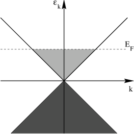
Figure 7: Single–particle energy spectrum of the Luttinger model. Occupied states are shown in grey, the dark grey area represents the states added to make the model solvable.

At least for weak interaction, this addition of extra states far from the Fermi energy is not expected to change the physics much. However, this modification makes the model exactly solvable even in the presence of nontrivial and possibly strong interactions. Moreover, and most importantly, many of the features of this model carry over even to strongly interacting fermions on a lattice.

We now introduce the Fourier components of the particle density operator for right and left movers:

$$\rho_{\pm}(q)=\sum_{k}a^{\dagger}_{\pm,k+q}a_{\pm,k},$$ (4.2)

The noninteracting Hamiltonian (and a more general model including interactions, see below) can be written in terms of these operators in a rather simple form and then be solved exactly. This is based on the following facts:

1. the density fluctuation operators $\rho_{\alpha}$, with $\alpha=\pm$, obey Bose type commutation relations:

   $$\left[\rho_{\alpha}(-q),\rho_{\alpha^{\prime}}(q^{\prime})\right]=\delta_{\alpha\alpha^{\prime}}\delta_{qq^{\prime}}\frac{\alpha qL}{2\pi}.$$ (4.3)

   The relation (4.3) for $q\neq q^{\prime}$ or $\alpha\neq\alpha^{\prime}$ can be derived by straightforward operator algebra. The slightly delicate part is eq.(4.3) for $q=q^{\prime}$. One easily finds

   $$[\rho_{+}(-q),\rho_{+}(q)]=\sum_{k}(\hat{n}_{k-q}-\hat{n}_{k})\;\;,$$ (4.4)

   where $\hat{n}_{k}$ is an occupation number operator. In a usual system with a finite interval of states between $-{k_{\rm F}}$ and ${k_{\rm F}}$ occupied, the summation index of one of the $\hat{n}$ operators could be shifted, giving a zero answer in eq.(4.4). In the present situation, with an infinity of states occupied below ${k_{\rm F}}$, this is not so. Consider for example the ground state and $q>0$. Then each term in eq.(4.4) with ${k_{\rm F}}<k<{k_{\rm F}}+q$ contributes unity to the sum, all other terms vanish, thus establishing the result (4.3). More generally, consider a state with all levels below a certain value $k_{0}$ ($<{k_{\rm F}}$) occupied, but an arbitrary number of particle hole pairs excited otherwise. One then has, assuming again $q>0$,

   $$\sum_{k}(\hat{n}_{k-q}-\hat{n}_{k}) = \left(\sum_{k\geq k_{0}}+\sum_{k<k_{0}}\right)(\hat{n}_{k-q}-\hat{n}_{k})$$ (4.5)

   $$= \sum_{k\geq k_{0}}(\hat{n}_{k-q}-\hat{n}_{k})$$

   $$= \sum_{k\geq k_{0}-q}\hat{n}_{k}-\sum_{k\geq k_{0}}\hat{n}_{k}$$

   $$= \sum_{k_{0}-q\leq k<k_{0}}\hat{n}_{k}=\frac{Lq}{2\pi}\;\;.$$

   The result is independent of $k_{0}$, and one thus can take the limit $k_{0}\rightarrow-\infty$. Together with an entirely parallel argument for $\rho_{-}$, this then proves eq.(4.3). Moreover, for $q>0$ both $\rho_{+}(-q)$ and $\rho_{-}(q)$ annihilate the noninteracting groundstate. One can easily recover canonical Bose commutation relations by introducing normalized operators, e.g. $\tilde{\rho}_{+}(q)=\sqrt{2\pi/(qL)}\rho_{+}(q)$ would be a canonical creation operator, but we won’t use this type of operators in the following.

2. The noninteracting Hamiltonian obeys a simple commutation relation with the density operators. For example

   $$\left[H_{0},\rho_{\alpha}(q)\right]=v_{{\mathrm{F}}}\alpha q\rho_{\alpha}(q)\;\;,$$ (4.6)

   i.e. states created by $\rho_{+}(q)$ are eigenstates of $H_{0}$, with energy $v_{{\mathrm{F}}}q$. Consequently, the kinetic part of the Hamiltonian can be re–written as a term bilinear in boson operators, i.e. quartic in fermion operators:

   $$H_{0}=\frac{2\pi v_{{\mathrm{F}}}}{L}\sum_{q>0,\alpha=\pm}\rho_{\alpha}(q)\rho_{\alpha}(-q)\;\;.$$ (4.7)

   This equivalence may be made more apparent noting that $\rho_{+}(q)$ creates particle–hole pairs that all have total momentum $q$. Their energy is $\varepsilon_{k+q}-\varepsilon_{k}$, which, because of the linearity of the spectrum, equals $v_{{\mathrm{F}}}q$, independently of $k$. Thus, states created by $\rho_{+}(q)$ are linear combinations of individual electron–hole excitations all with the same energy, and therefore are also eigenstates of (4.1).

3. The above point shows that the spectra of the bosonic and fermionic representations of $H_{0}$ are the same. To show complete equivalence, one also has to show that the degeneracies of all the levels are identical. This can be achieved calculating the partition function in the two representations and demonstrating that they are equal. This then shows that the states created by repeated application of $\rho_{\pm}$ on the ground state form a complete set of basis states [23, 24].

We now introduce interactions between the fermions. As long as only forward scattering of the type $(k_{{\mathrm{F}}};-k_{{\mathrm{F}}})\rightarrow(k_{{\mathrm{F}}};-k_{{\mathrm{F}}})$ or $(k_{{\mathrm{F}}};k_{{\mathrm{F}}})\rightarrow(k_{{\mathrm{F}}};k_{{\mathrm{F}}})$ is introduced, the model remains exactly solvable. The interaction Hamiltonian describing these processes takes the form

$$H_{\mathrm{int}}=\frac{1}{2L}\sum_{q,\alpha=\pm}\left(g_{2}(q)\rho_{\alpha}(q)\rho_{-\alpha}(-q)+g_{4}(q)\rho_{\alpha}(q)\rho_{\alpha}(-q)\right)\;\;.$$ (4.8)

Here, $g_{2}(q)$ and $g_{4}(q)$ are the Fourier transforms of a real space interaction potential, and in a realistic case one would of course have $g_{2}(q)=g_{4}(q)=g(q)$, but it is useful to allow for differences between $g_{2}$ and $g_{4}$. For Coulomb interactions one expects $g_{2},g_{4}>0$. In principle, the long–range part of the Coulomb repulsion leads to a singular $q$–dependence. Such singularities in the $g_{i}$ can be handled rather straightforwardly and can lead to interesting physical effects as will be discussed below. Here I shall limit myself to nonsingular $g_{2},g_{4}$. Electron–phonon interactions can lead to effectively attractive interactions between electrons, and therefore in the following I will not make any restrictive assumptions about the sign of the constants. One should however notice that a proper treatment of the phonon dynamics and of the resulting retardation effects requires more care [25].

Putting together (4.7) and (4.8), the complete interacting Hamiltonian, the Tomonaga–Luttinger model, then becomes a bilinear form in boson operators that is easily diagonalized by a Bogolyubov transformation. A first consequence is the expression for the excitation spectrum

$$\omega(q)=|q|\sqrt{\left(v_{{\mathrm{F}}}+\frac{g_{4}(q)}{2\pi}\right)^{2}-\left(\frac{g_{2}(q)}{2\pi}\right)^{2}}\;\;.$$ (4.9)

The diagonal boson operators are linear combinations of the original $\rho$ operators, and consequently, these elementary excitations are collective density oscillations, their energy being determined both by the kinetic energy term and the interactions.

We note here that in order for the Bogolyubov transformation to be a well–defined unitary transformation, $g_{2}(q)$ has to decrease at large $q$ at least as $|q|^{-1/2}$.[23] On the other hand, the large–$q$ behavior of $g_{2}$ is unimportant for the low–energy properties of the model. We therefore in the following will almost always use a $q$–independent $g_{2}$ and $g_{4}$. An approximate and frequently used way to cure the divergences arising due to this procedure is to keep a parameter $\alpha$ in subsequent formulae as a finite short–distance cutoff, of the order of a lattice spacing. One can then also include the “backward scattering” $(k_{{\mathrm{F}}};-k_{{\mathrm{F}}})\rightarrow(-k_{{\mathrm{F}}};k_{{\mathrm{F}}})$, because for spinless electron this is just the exchange analogue of forward scattering and does not constitute a new type of interaction. It is worthwhile emphasizing here that the solution is valid for arbitrarily strong interactions, no perturbative expansion is needed!

Up to this point, the construction does not allow for a direct calculation of correlation functions like the one–particle Green function or more generally any function involving individual creation or destruction operators. This type of correlation function becomes tractable by representing single particle operators in terms of the boson operators. To this end, we introduce the field operators

$$\phi(x) = -\frac{{\mathrm{i}}\pi}{L}\sum_{q\neq 0}\frac{1}{q}{\mathrm{e}}^{-\alpha|q|/2-{\mathrm{i}}qx}\left(\rho_{+}(q)+\rho_{-}(q)\right)-N\frac{\pi x}{L}\;\;,$$ (4.10)

$$\Pi(x) = \frac{1}{L}\sum_{q\neq 0}{\mathrm{e}}^{-\alpha|q|/2-{\mathrm{i}}qx}\left(\rho_{+}(q)-\rho_{-}(q)\right)+\frac{J}{L}$$ (4.12)

$$N=N_{+}+N_{-}\;\;,\quad J=N_{+}-N_{-}\;\;.$$

Here $N_{\pm}$ are the numbers of particles added to the ground state on the right– and left–moving branch i.e.

$$N_{\pm}=\rho_{\pm}(q=0)=\sum_{k}\left(\hat{n}_{\pm,k}-\langle\hat{n}_{\pm,k}\rangle_{0}\right).$$ (4.13)

Because addition of a particle changes both $N$ and $J$, one has the “selection rule” $(-1)^{N}=(-1)^{J}$; $\alpha$ is a cutoff parameter which (at least in principle, see the discussion above) has to be set to zero in the end of any calculation. The fields $\phi$ and $\Pi$ then obey canonical boson commutation relations:

$$[\phi(x),\Pi(y)]={\mathrm{i}}\delta(x-y)\;\;,$$ (4.14)

and $\phi$ is related to the local particle density via

$$\partial_{x}\phi=-\pi(\rho(x)-\rho_{0})\;\;,$$ (4.15)

where $\rho_{0}$ is the average particle density in the ground state. More precisely, in a lattice model this would represent the slowly varying components ($q\approx 0$) of the density, whereas components with $q\approx 2{k_{\rm F}}$ would correspond to crossproducts between $\psi_{\pm}$.

The expression for the single fermion operators then is

$$\psi_{\pm}(x)=\lim_{\alpha\rightarrow 0}\frac{1}{\sqrt{2\pi\alpha}}U_{\pm}\exp\left[\pm{\mathrm{i}}k_{{\mathrm{F}}}x\mp{\mathrm{i}}\phi(x)+{\mathrm{i}}\theta(x)\right]\;\;,$$ (4.16)

where the upper and lower sign refer to right– and left–moving electrons respectively, and

$$\theta(x) = \pi\int^{x}\Pi(x^{\prime})\,dx^{\prime}$$ (4.17)

$$= \frac{{\mathrm{i}}\pi}{L}\sum_{q\neq 0}\frac{1}{q}{\mathrm{e}}^{-\alpha|q|/2-{\mathrm{i}}qx}[\rho_{+}(q)-\rho_{-}(q)]+J\frac{\pi x}{L}\;\;.$$

The $U$–operators (sometimes referred to as “Klein factors”; they are non–Hermitian: $U_{\alpha}^{\dagger}\neq U_{\alpha}$) decrease the total particle number on one of the branches by unity and are necessary because the boson fields all conserve the total particle number. These operators also insure proper anticommutation between right- and left–going operators: one easily checks that the “chiral components” $\phi_{+}=\theta-\phi$ and $\phi_{-}=\theta+\phi$ commute with each other, one therefore needs the anticommutation relations $[U_{\alpha},U_{\beta}]_{+}=0$, etc. In the thermodynamic limit $L\rightarrow\infty$, the fact that the $U$’s change the particle number is of minor importance because this represents a shift of $k_{F}$ by a quantity of order $1/L$, and one then can replace the $U_{\alpha}$’s by Majorana (Hermitian) fermion operators obeying $[\eta_{\alpha},\eta_{\beta}]_{+}=0$,[26] as discussed in more detail in the appendix. In single–chain problems these effects play a minor role, however in the many chain systems to be discussed at the end of these notes, proper account of anticommutation is crucial.

A detailed derivation of the important eq.(4.16) as an operator identity is given in the literature [23, 24]. However, a simple plausibility argument can be given: creating a particle at site $x$ requires introducing a kink of height $\pi$ in $\phi$, i.e. $\phi$ has to be shifted by $\pi$ at points on the left of $x$. Displacement operators are exponentials of momentum operators, and therefore a first guess would be $\psi(x)\approx\exp({\mathrm{i}}\pi\int_{-\infty}^{x}\Pi(x^{\prime})dx^{\prime})$. However, this operator commutes with itself, instead of satisfying canonical anticommutation relations. Anticommutation is achieved by multiplying with an operator, acting at site $x$, that changes sign each time a particle passes through $x$. Such an operator is $\exp(\pm{\mathrm{i}}\phi(x))$. The product of these two factors then produces (4.16).

The full Hamiltonian can also be simply expressed in terms of $\phi$ and $\Pi$. In the long–wavelength limit, neglecting the momentum dependence of the $g_{i}$, one can express the total Hamiltonian in the field phase formalism

$$H=H_{0}+H_{\mathrm{int}}=\int dx\left(\frac{\pi uK}{2}\Pi(x)^{2}+\frac{u}{2\pi K}(\partial_{x}\phi)^{2}\right)\;\;.$$ (4.18)

This is obviously just the Hamiltonian of an elastic string, with the eigenmodes corresponding to the collective density fluctuations of the fermion liquid. It is important to notice that these collective modes are the only (low–energy) excited states, and that in particular there are no well–defined single particle excitations, nor are there the incoherent particle–hole pair excitations typical of a Fermi gas. The parameters in (4.18) are given by

$$u=\sqrt{\left(v_{{\mathrm{F}}}+\frac{g_{4}}{2\pi}\right)^{2}-\left(\frac{g_{2}}{2\pi}\right)^{2}}\;\;,\;K=\sqrt{\frac{2\pi v_{{\mathrm{F}}}+g_{4}-g_{2}}{2\pi v_{{\mathrm{F}}}+g_{4}+g_{2}}}\;\;.$$ (4.19)

The energies of the eigenstates are $\omega(q)=u|q|$, in agreement with eq. (4.9). From the continuity equation, the expression (4.15) for the local particle density and the equation of motion of $\phi$ the (number) current density is

$$j(x)=uK\Pi(x)\;\;.$$ (4.20)

Note in particular that for $g_{2}=g_{4}$ one has $uK=v_{{\mathrm{F}}}$, i.e. the expression for the current density is interaction–independent. The relation $uK=v_{{\mathrm{F}}}$ holds in particular for systems with full (Galilean) translational invariance. On the other hand, in the continuum limit of lattice systems this relation is in general not true.

The most remarkable result here is the “collectivization” of the dynamics: there are no quasiparticle–like excitations. In fact there is a rather simple physical picture explaining this: imagine accelerating one particle a little bit in one direction. Very soon it will hit its neighbor and transmit its momentum to it, and the neighbor will in turn transmit its momentum to a further neighbor, and so on. Quite quickly, the initial localized motion will have spread coherently through the whole system. This picture can be formalized noting that in one dimension the difference between a solid and a fluid is not well–defined: whereas is higher dimensions solids and fluids are differentiated by the presence or absence of long–wavelength transverse modes, no transverse modes can exist in a system with movement along only one direction. The long–wavelength modes thus can equally well be considered as the phonons of a one–dimensional crystal [27, 28]. Note that on the contrary in dimensions larger than one the neighbors of any given particle can be pushed aside, giving rise to a backflow that allows the particle to move trough the system more or less freely.

The exclusive existence of collective excitations, at least at low energies, is one of the typical properties of the Luttinger liquid. Rather than discussing the physics of the spinless case in detail, we will turn now to the more interesting case of fermions with spin.

4.2 Model with spin; the concept of the Luttinger Liquid

In the case of spin–1/2 fermions, all the fermion operators acquire an additional spin index $s$. Following the same logic as above, the kinetic energy then takes the form

$$H_{0} = v_{{\mathrm{F}}}\sum_{k,s}\left((k-k_{{\mathrm{F}}})a_{+,k,s}^{\dagger}a_{+,k,s}+(-k-k_{{\mathrm{F}}})a_{-,k,s}^{\dagger}a^{\phantom{\dagger}}_{-,k,s}\right)$$ (4.21)

$$= \frac{2\pi v_{{\mathrm{F}}}}{L}\sum_{q>0,\alpha=\pm,s}\rho_{\alpha,s}(q)\rho_{\alpha,s}(-q)\;\;,$$

where density operators for spin projections $s=\uparrow,\downarrow$ have been introduced:

$$\rho_{\pm,s}(q)=\sum_{k}a^{\dagger}_{\pm,k+q,s}a_{\pm,k,s}.$$ (4.22)

There are now two types of interaction. First, the “backward scattering” $(k_{{\mathrm{F}}},s;-k_{{\mathrm{F}}},t)$ $\rightarrow$ $(-k_{{\mathrm{F}}},s;k_{{\mathrm{F}}},t)$ which for $s\neq t$ cannot be re–written as an effective forward scattering (contrary to the spinless case). The corresponding Hamiltonian is

$$H_{\mathrm{int},1}=\frac{1}{L}\sum_{k,p,q,s,t}g_{1}a_{+,k,s}^{\dagger}a_{-,p,t}^{\dagger}a^{\phantom{\dagger}}_{+,p+2k_{{\mathrm{F}}}+q,t}a^{\phantom{\dagger}}_{-,k-2k_{{\mathrm{F}}}-q,s}\;\;.$$ (4.23)

And, of course, there is also the forward scattering, of a form similar to the spinless case

$$H_{\mathrm{int},2} = \frac{1}{2L}\sum_{q,\alpha,s,t}\left(g_{2}(q)\rho_{\alpha,s}(q)\rho_{-\alpha,t}(-q)+g_{4}(q)\rho_{\alpha,s}(q)\rho_{\alpha,t}(-q)\right)\;\;.$$ (4.24)

To go to the bosonic description, one introduces $\phi$ and $\Pi$ fields for the two spin projections separately, and then transforms to charge and spin bosons via $\phi_{\rho,\sigma}=(\phi_{\uparrow}\pm\phi_{\downarrow})/\sqrt{2}$, $\Pi_{\rho,\sigma}=(\Pi_{\uparrow}\pm\Pi_{\downarrow})/\sqrt{2}$. The operators $\phi_{\nu}$ and $\Pi_{\nu}$ obey Bose–like commutation relations:

$$[\phi_{\nu}(x),\Pi_{\mu}(y)]={\mathrm{i}}\delta_{\nu\mu}\delta(x-y)\;\;,$$ (4.25)

and single fermion operators can be written in a form analogous to (4.16):

$$\psi_{\pm,s}(x)=\lim_{\alpha\rightarrow 0}\frac{\eta_{\pm,s}}{\sqrt{2\pi\alpha}}\exp\left({\pm{\mathrm{i}}k_{{\mathrm{F}}}x}-{\mathrm{i}}(\pm(\phi_{\rho}+s\phi_{\sigma})+(\theta_{\rho}+s\theta_{\sigma}))/\sqrt{2}\right)\;\;,$$ (4.26)

where $\theta_{\nu}(x)=\pi\int^{x}\Pi_{\nu}(x^{\prime})dx^{\prime}$.

The full Hamiltonian $H=H_{0}+H_{int,1}+H_{int,2}$ then takes the form

$$H=H_{\rho}+H_{\sigma}+\frac{2g_{1}}{(2\pi\alpha)^{2}}\int dx\cos(\sqrt{8}\phi_{\sigma})\;\;.$$ (4.27)

Here $\alpha$ is a short–distance cutoff, and for $\nu=\rho,\sigma$

$$H_{\nu}=\int dx\left(\frac{\pi u_{\nu}K_{\nu}}{2}\Pi_{\nu}^{2}+\frac{u_{\nu}}{2\pi K_{\nu}}(\partial_{x}\phi_{\nu})^{2}\right)\;\;,$$ (4.28)

with

$$u_{\nu}=\sqrt{\left(v_{{\mathrm{F}}}+\frac{g_{4,\nu}}{\pi}\right)^{2}-\left(\frac{g_{\nu}}{2\pi}\right)^{2}}\;\;,\;K_{\nu}=\sqrt{\frac{2\pi v_{{\mathrm{F}}}+2g_{4,\nu}+g_{\nu}}{2\pi v_{{\mathrm{F}}}+2g_{4,\nu}-g_{\nu}}}\;\;,$$ (4.29)

and $g_{\rho}=g_{1}-2g_{2}$, $g_{\sigma}=g_{1}$, $g_{4,\rho}=g_{4}$, $g_{4,\sigma}=0$. The choice of sign (which is the conventional one) for the cosine–term in eq.(4.27) corresponds to a particular “gauge choice”, as discussed in the appendix.

For a noninteracting system one thus has $u_{\nu}=v_{{\mathrm{F}}}$ (charge and spin velocities equal!) and $K_{\nu}=1$. For $g_{1}=0$, (4.27) describes independent long-wavelength oscillations of the charge and spin density, with linear dispersion relation $\omega_{\nu}(k)=u_{\nu}|k|$, and the system is conducting. As in the spinless case, there are no single–particle or single particle–hole pair excited states. This model (no backscattering), usually called the Tomonaga–Luttinger model, is the one to which the bosonization method was originally applied [20, 21, 29].

For $g_{1}\neq 0$ the cosine term has to be treated perturbatively. We have already obtained the corresponding renormalization group equations in the previous section (eq.(3.23)). In particular, for repulsive interactions ($g_{1}>0$), $g_{1}$ is renormalized to zero in the long-wavelength limit, and at the fixed point one has $K_{\sigma}^{*}=1$. The three remaining parameters in (4.27) then completely determine the long-distance and low–energy properties of the system.

It should be emphasized that (4.27) has been derived here for fermions with linear energy–momentum relation. For more general (e.g. lattice) models, there are additional operators arising from band curvature and the absence of high–energy single–particle states [23]. One can however show that all these effects are, at least for not very strong interaction, irrelevant in the renormalization group sense, i.e. they do not affect the low–energy physics. Thus, (4.27) is still the correct effective Hamiltonian for low–energy excitations. The lattice effects however intervene to give rise to “higher harmonics” in the expression for the single–fermion operators, i.e. there are low energy contributions at wavenumbers $q\approx(2m+1)k_{{\mathrm{F}}}$ for arbitrary integer $m$ [27].

The Hamiltonian (4.27) also provides an explanation for the physics of the case of negative $g_{1}$, where the renormalization group scales to strong coupling (eq.(3.23)). In fact, if $|g_{1}|$ is large in (4.27), it is quite clear that the elementary excitations of $\phi_{\sigma}$ will be small oscillations around one of the minima of the cosine term, or possibly soliton–like objects where $\phi_{\sigma}$ goes from one of the minima to the other. Both types of excitations have a gap, i.e. for $g_{1}<0$ one has a gap in the spin excitation spectrum, whereas the charge excitations remain massless. This can actually investigated in more detail in an exactly solvable case [30]. We will subsequently concentrate on the case $g_{1}>0$, so that there is no spin gap, however investigations of spectral functions as described below have also been recently performed for the case with a spin gap.[31]

4.2.1 Spin–charge separation

One of the more spectacular consequences of the Hamiltonian (4.27) is the complete separation of the dynamics of the spin and charge degrees of freedom. For example, in general one has $u_{\sigma}\neq u_{\rho}$, i.e. the charge and spin oscillations propagate with different velocities. Only in a noninteracting system or if some accidental degeneracy occurs one does have $u_{\sigma}=u_{\rho}=v_{{\mathrm{F}}}$. To make the meaning of this fact more transparent, let us create an extra particle in the ground state, at $t=0$ and spatial coordinate $x_{0}$. The charge and spin densities then are easily found, using $\rho(x)=-(\sqrt{2}/\pi)\partial_{x}\phi_{\rho}$ (note that $\rho(x)$ is the deviation of the density from its average value) and $\sigma_{z}(x)=-(\sqrt{2}/\pi)\partial_{x}\phi_{\sigma}$ :

$$\langle 0|\psi_{+}(x_{0})\rho(x)\psi^{\dagger}_{+}(x_{0})|0\rangle = \delta(x-x_{0})\;\;,$$

$$\langle 0|\psi_{+}(x_{0})\sigma_{z}(x)\psi^{\dagger}_{+}(x_{0})|0\rangle = \delta(x-x_{0})\;\;.$$ (4.30)

Now, consider the time development of the charge and spin distributions. The time–dependence of the charge and spin density operators is easily obtained from (4.27) (using the fixed point value $g_{1}=0$), and one obtains

$$\langle 0|\psi_{+}(x_{0})\rho(x,t)\psi^{\dagger}_{+}(x_{0})|0\rangle = \delta(x-x_{0}-u_{\rho}t)\;\;,$$

$$\langle 0|\psi_{+}(x_{0})\sigma_{z}(x,t)\psi^{\dagger}_{+}(x_{0})|0\rangle = \delta(x-x_{0}-u_{\sigma}t)\;\;.$$ (4.31)

Because in general $u_{\sigma}\neq u_{\rho}$, after some time charge and spin will be localized at completely different points in space, i.e. charge and spin have separated completely.

Here a linear energy–momentum relation has been assumed for the electrons, and consequently the shape of the charge and spin distributions is time–independent. If the energy–momentum relation has some curvature (as is necessarily the case in lattice systems) the distributions will widen with time. However this widening is proportional to $\sqrt{t}$, and therefore much smaller than the distance between charge and spin. Thus, the qualitative picture of spin-charge separation is unchanged.

4.2.2 Physical properties

The simple form of the Hamiltonian (4.27) at the fixed point $g_{1}^{*}=0$ makes the calculation of physical properties rather straightforward. The specific heat now is determined both by the charge and spin modes, and consequently the specific heat coefficient $\gamma$ is given by

$$\gamma/\gamma_{0}=\frac{1}{2}(v_{{\mathrm{F}}}/u_{\rho}+v_{{\mathrm{F}}}/u_{\sigma})\;\;.$$ (4.32)

Here $\gamma_{0}$ is the specific heat coefficient of noninteracting electrons of Fermi velocity $v_{{\mathrm{F}}}$.

The spin susceptibility and the compressibility are equally easy to obtain. Note that in (4.27) the coefficient $u_{\sigma}/K_{\sigma}$ determines the energy necessary to create a nonzero spin polarization, and, as in the spinless case, $u_{\rho}/K_{\rho}$ fixes the energy needed to change the particle density. Given the fixed point value $K_{\sigma}^{*}=1$, one finds

$$\chi/\chi_{0}=v_{{\mathrm{F}}}/u_{\sigma}\;\;,\quad\kappa/\kappa_{0}=v_{{\mathrm{F}}}K_{\rho}/u_{\rho}\;\;,$$ (4.33)

where $\chi_{0}$ and $\kappa_{0}$ are the susceptibility and compressibility of the noninteracting case. From eqs.(4.32) and (4.33) the Wilson ratio is

$$R_{\mathrm{W}}=\frac{\chi}{\gamma}\frac{\gamma_{0}}{\chi_{0}}=\frac{2u_{\rho}}{u_{\rho}+u_{\sigma}}\;\;.$$ (4.34)

The quantity $\Pi_{\rho}(x)$ is proportional to the current density. As before, the Hamiltonian commutes with the total current, one thus has

$$\sigma(\omega)=2K_{\rho}u_{\rho}\delta(\omega)+\sigma_{\mathrm{reg}}(\omega)\;\;,$$ (4.35)

i.e. the product $K_{\rho}u_{\rho}$ determines the weight of the dc peak in the conductivity. If the total current commutes with the Hamiltonian $\sigma_{\mathrm{reg}}$ vanishes, however more generally this part of the conductivity varies as $\omega^{3}$ at low frequencies [32].

The above properties, linear specific heat, finite spin susceptibility, and dc conductivity are those of an ordinary Fermi liquid, the coefficients $u_{\rho},u_{\sigma}$, and $K_{\rho}$ determining renormalizations with respect to noninteracting quantities. However, the present system is not a Fermi liquid. This is in fact already obvious from the preceding discussion on charge–spin separation, and can be made more precise considering the single–particle Green function. Using the representation (4.26) of fermion operators one finds (at the fixed point $g_{1}=0$)

$$G^{{\mathrm{R}}}(x,t) = -{\mathrm{i}}\Theta(t)\left\langle\left[\psi_{+,s}(x,t),\psi_{+,s}^{\dagger}(0,0)\right]_{+}\right\rangle$$

$$= -\frac{\Theta(t)}{\pi}{\mathrm{e}}^{{\mathrm{i}}k_{{\mathrm{F}}}x}{\rm Re}\left(\frac{1}{\sqrt{(u_{\rho}t-x)(u_{\sigma}t-x)}}\left[\frac{\alpha^{2}}{(\alpha+{\mathrm{i}}u_{\rho}t)^{2}+x^{2}}\right]^{\delta/2}\right),$$ (4.36)

where the presence of the Heaviside function ensures the retarded nature of $G^{{\mathrm{R}}}$ and $[,]_{+}$ denotes the anticommutation of fermion operators. Note that this expression factorizes into a spin and a charge contribution which propagate with different velocities. Fourier transforming (4.36) gives the momentum distribution function in the vicinity of $k_{{\mathrm{F}}}$:

$$n_{k}\approx n_{k_{{\mathrm{F}}}}-{\rm const.}\times{\rm sign}(k-k_{{\mathrm{F}}})|k-k_{{\mathrm{F}}}|^{\delta}\;\;\;\;,$$ (4.37)

and for the single-particle density of states (i.e. the momentum–integrated spectral density) one finds:

$$N(\omega)\approx|\omega|^{\delta}\;\;.$$ (4.38)

In both cases $\delta=(K_{\rho}+1/K_{\rho}-2)/4$. Note that for any $K_{\rho}\neq 1$, i.e. for any nonvanishing interaction, the momentum distribution function and the density of states have power–law singularities at the Fermi level, with a vanishing single particle density of states at $E_{{\mathrm{F}}}$. This behavior is obviously quite different from a standard Fermi liquid which would have a finite density of states and a step–like singularity in $n_{k}$. The absence of a step at $k_{{\mathrm{F}}}$ in the momentum distribution function implies the absence of a quasiparticle pole in the one–particle Green function. In fact, a direct calculation of the spectral function $A(k,\omega)$ from (4.36) [33, 34] shows that the usual quasiparticle pole is replaced by a continuum, with a lower threshold at $\min_{\nu}(u_{\nu}(k-k_{{\mathrm{F}}}))$ and branch cut singularities at $\omega=u_{\rho}p$ and $\omega=u_{\sigma}p$:

$$A(k,\omega) \approx(\omega-u_{\sigma}(k-k_{{\mathrm{F}}}))^{\delta-1/2} \left|\omega-u_{\rho}(k-k_{{\mathrm{F}}})\right|^{(\delta-1)/2}\quad(u_{\rho}>u_{\sigma})\;\;,$$ (4.39)

$$A(k,\omega) \approx(\omega-u_{\rho}(k-k_{{\mathrm{F}}}))^{(\delta-1)/2} \left|\omega-u_{\sigma}(k-k_{{\mathrm{F}}})\right|^{\delta-1/2}\quad(u_{\rho}<u_{\sigma})\;\;.$$ (4.40)

The coefficient $K_{\rho}$ also determines the long-distance decay of all other correlation functions of the system: Using the representation (4.26) the charge and spin density operators at $2k_{{\mathrm{F}}}$ are

$$O_{\mathrm{CDW}}(x) = \sum_{s}\psi_{-,s}^{\dagger}(x)\psi_{+,s}(x)$$ (4.41)

$$= \lim_{\alpha\rightarrow 0}\frac{{\mathrm{e}}^{2{\mathrm{i}}k_{{\mathrm{F}}}x}}{\pi\alpha}{\mathrm{e}}^{-{\mathrm{i}}\sqrt{2}\phi_{\rho}(x)}\cos[\sqrt{2}\phi_{\sigma}(x)]\;\;,$$

$$O_{{\mathrm{SDW}}_{x}}(x) = \sum_{s}\psi_{-,s}^{\dagger}(x)\psi_{+,-s}(x)$$ (4.42)

$$= \lim_{\alpha\rightarrow 0}\frac{{\mathrm{e}}^{2{\mathrm{i}}k_{{\mathrm{F}}}x}}{\pi\alpha}{\mathrm{e}}^{-{\mathrm{i}}\sqrt{2}\phi_{\rho}(x)}\cos[\sqrt{2}\theta_{\sigma}(x)]\;\;.$$

Similar relations are also found for other operators. It is important to note here that all these operators decompose into a product of one factor depending on the charge variable only by another factor depending only on the spin field. Using the Hamiltonian (4.27) at the fixed point $g_{1}^{*}=0$ one finds for example for the charge and spin correlation functions

$$\langle n(x)n(0)\rangle = K_{\rho}/(\pi x)^{2}+A_{1}\cos(2k_{{\mathrm{F}}}x)x^{-1-K_{\rho}}\ln^{-3/2}(x)$$

$$\mbox{}+A_{2}\cos(4k_{{\mathrm{F}}}x)x^{-4K_{\rho}}+\ldots\;\;,$$ (4.43)

$$\langle{\mathbf{S}}(x)\cdot{\mathbf{S}}(0)\rangle = 1/(\pi x)^{2}+B_{1}\cos(2k_{{\mathrm{F}}}x)x^{-1-K_{\rho}}\ln^{1/2}(x)+\ldots\;\;,$$ (4.44)

with model dependent constants $A_{i},B_{i}$. The ellipses in (4.43) and (4.44) indicate higher harmonics of $\cos(2k_{{\mathrm{F}}}x)$ which are present but decay faster than the terms shown here. Similarly, correlation functions for singlet (SS) and triplet (TS) superconducting pairing are

$$\langle O^{\dagger}_{\mathrm{SS}}(x)O_{\mathrm{SS}}(0)\rangle = Cx^{-1-1/K_{\rho}}\ln^{-3/2}(x)+\ldots\;\;,$$

$$\langle O^{\dagger}_{\mathrm{TS}_{\alpha}}(x)O_{\mathrm{TS}_{\alpha}}(0)\rangle = Dx^{-1-1/K_{\rho}}\ln^{1/2}(x)+\dots\;\;.$$ (4.45)

The logarithmic corrections in these functions [36] have been studied in detail recently [37, 38, 39, 40]. The corresponding susceptibilities (i.e. the Fourier transforms of the above correlation functions) behave at low temperatures as

$$\chi_{\mathrm{CDW}}(T)\approx T^{K_{\rho}-1}|\ln(T)|^{-3/2} \;\;, \chi_{\mathrm{SDW}}(T)\approx T^{K_{\rho}-1}|\ln(T)|^{1/2}\;\;,$$ (4.46)

$$\chi_{\mathrm{SS}}(T)\approx T^{1/K_{\rho}-1}|\ln(T)|^{-3/2} \;\;, \chi_{\mathrm{TS}}(T)\approx T^{1/K_{\rho}-1}|\ln(T)|^{1/2}\;\;,$$ (4.47)

i.e. for $K_{\rho}<1$ (spin or charge) density fluctuations at $2k_{{\mathrm{F}}}$ are enhanced and diverge at low temperatures, whereas for $K_{\rho}>1$ pairing fluctuations dominate. The “phase diagram”, showing in which part of parameter space which type of correlation diverges for $T\rightarrow 0$ is shown in fig.8.

Figure 8: Phase diagram for interacting spin–$1/2$ fermions.

These correlation functions with their power law variations actually determine experimentally accessible quantities: the $2k_{{\mathrm{F}}}$ and $4k_{{\mathrm{F}}}$ charge correlations lead to X–ray scattering intensities $I_{2k_{{\mathrm{F}}}}\approx T^{K_{\rho}}$, $I_{4k_{{\mathrm{F}}}}\approx T^{4K_{\rho}-1}$, and similarly the NMR relaxation rate due to $2k_{{\mathrm{F}}}$ spin fluctuations varies as $1/T_{1}\approx T^{K_{\rho}}$. The remarkable fact in all the above results is that there is only one coefficient, $K_{\rho}$, which determines all the asymptotic power laws.

We here re–emphasize the two important properties of spin–1/2 interacting fermions in one dimension: (i) correlation functions show power–law decay, with interaction–dependent powers determined by one coefficient, $K_{\rho}$; and (ii) “spin–charge separation”: spin and charge degrees of freedom propagate with different velocities. Both these properties are typical of the Luttinger liquid and invalidate the Landau quasiparticle concept in one dimension.

A nice experimental example of different spin–charge separation (different velocities for the spin and charge modes) is provided by Raman scattering experiments on single–channel quantum wires.[41, 42, 43] On the other hand, the situation in quasi–one–dimensional conductors [44] is less clear: in compounds of the TTF–TCNQ series, the observation of strong $4k_{F}$ CDW fluctuations [45] seems only to be explainable in the Luttinger–liquid picture. On the other hand, in the much studies $\rm(TMTSF)_{2}X$ family of compounds, the NMR data can be interpreted in the Luttinger liquid framework [46], but much of the magnetotransport work of Chaikin and collaborators is explained rather satisfactorily using a Fermi liquid like picture.

4.2.3 Long–range interactions: Wigner crystallization

The above calculations can be straightforwardly generalized to the case of long–range interactions. Of interest is the case of unscreened Coulomb interactions ($V(r)=e^{2}/r$) which for example is of relevance for the physics of an isolated quantum wire. The short–distance singularity has to be cut off, and for example in a wire of diameter $d$ an approximate form would be $V(r)=e^{2}/\sqrt{x^{2}+d^{2}}$, leading to a Fourier transform $V(q)=2e^{2}K_{0}(qd)$. The long–range nature of the interaction is only of importance for the forward–scattering processes, and these appear only in the charge part of the Hamiltonian which is now given by

$$H_{\rho} = \frac{v_{{\mathrm{F}}}}{2\pi}\int dx\left(\pi^{2}(1+\tilde{g}_{1})\Pi_{\rho}^{2}+(1-\tilde{g}_{1})(\partial_{x}\phi_{\rho})^{2}\right)$$ (4.48)

$$+\frac{1}{\pi^{2}}\int dxdx^{\prime}V(x-x^{\prime})\partial_{x}\phi_{\rho}\partial_{x^{\prime}}\phi_{\rho}\;\;,$$

where $\tilde{g}_{1}=g_{1}/(2\pi v_{{\mathrm{F}}})$. The elementary excitations then are found to be charge oscillations (plasmons), with energy–momentum relation

$$\omega_{\rho}(q)=v_{{\mathrm{F}}}|q|\sqrt{(1+\tilde{g}_{1})(1-\tilde{g}_{1}+2\tilde{V}(q))}$$ (4.49)

where $\tilde{V}(q)=V(q)/(\pi v_{{\mathrm{F}}})$. The long–wavelength form ($q\to 0$), $\omega_{\rho}(q)\approx|q^{2}\ln q|^{1/2}$, agrees with RPA calculations [47, 48], however, the effect of $g_{1}$, which is a short–range exchange contribution, are usually neglected in those calculations. The spin modes are still given by $\omega_{\sigma}(q)=u_{\sigma}|q|$, with $u_{\sigma}=v_{{\mathrm{F}}}\sqrt{1-\tilde{g}_{1}^{2}}$.

In the evaluation of correlation functions, the charge averages lead to

$$\langle(\phi_{\rho}(x)-\phi_{\rho}(0))^{2}\rangle = \int_{0}^{\infty}dq\,\frac{1-\cos qx}{q}\sqrt{\frac{1+\tilde{g}_{1}}{1-\tilde{g}_{1}+2\tilde{V}(q)}}$$ (4.50)

$$\approx c_{2}\sqrt{\ln x}\;\;,$$

with $c_{2}=\sqrt{(1+\tilde{g}_{1})\pi v_{{\mathrm{F}}}/e^{2}}$. One thus obtains for example

$$\langle\rho(x)\rho(0)\rangle = A_{1}\cos(2k_{{\mathrm{F}}}x)\exp(-c_{2}\sqrt{\ln x})/x$$ (4.51)

$$+A_{2}\cos(4k_{{\mathrm{F}}}x)\exp(-4c_{2}\sqrt{\ln x})+...\;\;,$$

where $A_{1,2}$ are interaction dependent constants, and only the most slowly decaying Fourier components are exhibited. The most interesting point here is the extremely slow decay (much slower than any power law!) of the $4k_{{\mathrm{F}}}$ component, showing an incipient charge density wave at wavevector $4k_{{\mathrm{F}}}$. This slow decay should be compared with the power–law decay found for short–range interactions (eq.(4.43)). The $4k_{{\mathrm{F}}}$ oscillation period is exactly the average interparticle spacing, i.e. the structure is that expected for a one–dimensional Wigner crystal. Of course, because of the one–dimensional nature of the model, there is no true long–range order, however, the extremely slow decay of the $4k_{{\mathrm{F}}}$ oscillation would produce strong quasi–Bragg peaks in a scattering experiment. It is worthwhile to point out that this $4k_{{\mathrm{F}}}$ contribution arises even if the Coulomb interaction is extremely weak and depends only on the long–range character of the interaction. On the other hand, any $2k_{{\mathrm{F}}}$ scattering is considerably weaker, due to the $1/x$ prefactor in (4.51) which has its origin in the contribution of spin fluctuations. The $2{k_{\rm F}}$ spin correlations equally contain a $1/x$ factor and thus have the same asymptotic decay as the $2{k_{\rm F}}$ charge correlations, eq.(4.51). On the other hand, correlation functions that involve operators changing the total number of particles (e.g. the single particle Green function and pairing correlation functions) decay like $\exp[-{\mathrm{cst.}}\times(\ln x)^{-3/2}]$, i.e. faster than any power law. This in particular means that the momentum distribution function $n_{k}$ and all its derivatives are continuous at $k_{{\mathrm{F}}}$, and there is only an essential singularity at $k_{{\mathrm{F}}}$.

It is instructive to compare the above result (4.51), obtained in the limit of weak Coulomb interactions, with the case of strong repulsion (or, equivalently, heavy particles). The configuration of minimum potential energy is one of a chain of equidistant particles with lattice constant $a$, and quantum effects are expected to lead only to small oscillations in the distances between particles. The Hamiltonian then is

$$H=\sum_{l}\frac{p_{l}^{2}}{2m}+\frac{1}{4}\sum_{l\neq m}V^{\prime\prime}(ma)(u_{l}-u_{l+m})^{2}\;\;,$$ (4.52)

where $u_{l}$ is the deviation of particle $l$ from its equilibrium position. In the long–wavelength limit, the oscillation of this lattice have energy $\omega(q)=\sqrt{2/(ma)}eq|\ln(qa)|^{1/2}$. The most slowly decaying part of the density–density correlation function then is

$$\langle\rho(x)\rho(0)\rangle\approx\cos(2\pi x/a)\exp\left(-\frac{4\pi}{(2me^{2}a)^{1/2}}\sqrt{\ln x}\right).$$ (4.53)

Noticing that $k_{{\mathrm{F}}}=\pi/(2a)$, one observes that the results (4.51) and (4.53) are (for $g_{1}=0$) identical as far as the long–distance asymptotics are concerned, including the constants in the exponentials. Eq. (4.51) was obtained in the weak interaction limit, whereas (4.53) applies for strong Coulomb forces. Similarly, the small–$q$ limit of the charge excitation energies is identical.

4.3 Summary

In this section we have developed the basic bosonization formalism for one–dimensional interacting fermions and seen some elementary and direct applications to the calculation of some physical properties, in particular correlation functions. We have seen that the properties of the one–dimensional interacting system, the Luttinger liquid, are fundamentally different from two- or three–dimensional Fermi liquids. In particular the elementary excitations are not quasiparticles but rather collective oscillations of the charge and spin density, propagating coherently, but in general at different velocities. This gives rise to the interesting phenomenon of spin–charge separation. Finally, and again contrary to the Fermi–liquid case, most correlation functions show non–universal powerlaws, with interaction–dependent exponents. However, all these exponents depend only on one parameter, $K_{\rho}$, the spin analogue of which, $K_{\sigma}$, being fixed to unity by spin–rotation invariance ($K_{\sigma}\neq 1$ is possible if spin rotation invariance is broken). Beyond $K_{\rho}$, the only parameters that intervene in the low–energy physics of a Luttinger liquid are the velocities of the spin and charge modes, $u_{\rho,\sigma}$. In the spinless case only two parameters, $K$ and $u$ are involved. Finally, we have seen that long–range (Coulomb) interactions can profoundly modify these properties.

For lack of time and space, we have not touched here upon a number of interesting uses and generalizations of the bosonization method, in particular the Kondo effect [49] and applications to Fermi systems in more than one dimension.[50, 51] An extensive recent review on Luttinger liquids and bosonization has been given by Voit.[52]

5 Applications

We will subsequently discuss some results from applications of the formalism developed to interesting physical questions: transport and the effect of disorder, and the physics of antiferromagnetic spin chains. Here, we will come across the two cases where Luttinger liquid behavior is probably best established experimentally: the physics of quantum Hall edge states, upon which we will only touch briefly, and quantum spin systems, in particular the spin-$1/2$ antiferromagnet, which we will discuss in some detail, with some reference to experiment.

5.1 Transport

5.1.1 Conductivity and conductance

In the previous section we were concerned with equilibrium properties and correlation functions, in order to characterize the different phases possible in a one–dimensional system of interacting fermions. Here, we will investigate transport, in particular the dc conductivity. Finite–frequency effects have also been investigated, and the reader is referred to the literature [32, 53].

To clarify some of the basic notions, let us first consider a Luttinger model in the presence of a weak space– and time–dependent external potential $\varphi$. The interaction of the fermions with $\varphi$ is described by the extra term

$$H_{\mathrm{ext}}=-e\int dx\hat{\rho}(x)\varphi(x,t)$$ (5.1)

in the total Hamiltonian. We will assume that the external field is slowly varying in space, so that in the particle–density operator $\hat{\rho}$ only products of either two right– or two left–going fermion operators appear but no cross terms. Standard linear response theory tells us that the current induced by the potential is given by

$$j(x,t)=-\frac{e^{2}}{\hbar}\int_{-\infty}^{t}dt^{\prime}\int dx^{\prime}D_{j\rho}(x-x^{\prime},t-t^{\prime})\varphi(x^{\prime},t^{\prime})\;\;,$$ (5.2)

where the retarded current–density correlation function is given by

$$D_{j\rho}(x,t) = -{\mathrm{i}}\Theta(t)\langle[j(x,t),\rho(0,0)]\rangle$$ (5.3)

$$= -\frac{u_{\rho}K_{\rho}}{\pi}\Theta(t)\left(\delta^{\prime}(x-u_{\rho}t)+\delta^{\prime}(x+u_{\rho}t)\right)\;\;.$$

The second line is the result for spin–$1/2$ electrons. For spinless fermions one has to make the replacement $u_{\rho}K_{\rho}\rightarrow uK/2$.

Let us now first consider the situation where we adiabatically switch on a potential of frequency $\omega$ and wavenumber $q$ along the whole length of the system. From eq.(5.3) one then straightforwardly obtains the $q$– and $\omega$–dependent conductivity as

$$\sigma(q,\omega)=\frac{4e^{2}}{\hbar}u_{\rho}K_{\rho}\frac{{\mathrm{i}}(\omega+{\mathrm{i}}0^{+})}{(\omega+{\mathrm{i}}0^{+})^{2}-u_{\rho}^{2}q^{2}}\;\;.$$ (5.4)

In particular, the real part of the conductivity for constant applied field is

$${\rm Re}\,\sigma(0,\omega)=\frac{2e^{2}}{\hbar}u_{\rho}K_{\rho}\delta(\omega)\;\;,$$ (5.5)

in agreement with eq.(4.35) (where units with $e^{2}=\hbar=1$ were used).

Applying on the other hand a static field over a finite part of the sample, one obtains a current $j=2e^{2}K_{\rho}U/h$, where $U$ is the applied tension. The conductance thus is

$$G=\frac{2e^{2}}{h}K_{\rho}\;\;,$$ (5.6)

and depends on $K_{\rho}$ only, not on $u_{\rho}$. For the noninteracting case $K_{\rho}=1$ this is Landauer’s well–known result [54]. Note that interactions affect the value of the conductance. The conductance here is independent on the length over which the field is applied. Noting that in dimension $d$ the conductance is related to the dc conductivity via $G=L^{d-2}\sigma$, a length–independent conductance implies an infinite conductivity in one dimension, in agreement with eq.(5.3). The fact that $u_{\rho}$ does not appear in the expression for $G$ can be understood noting that applying a static field over a finite (but large) part of the sample, one is essentially studying the wavenumber–dependent conductivity at strictly zero frequency, which from eq.(5.20) is given by $\sigma(q,0)=2e^{2}K_{\rho}\delta(q)/\hbar$, indeed independent on $u_{\rho}$. On the other hand, applying a field of finite frequency over a finite length $\ell$, one can see that one measures the conductivity $\sigma(q\rightarrow 0,\omega)$ if $\omega>u_{\rho}/\ell$.

The situation of a finite static potential drop over only a finite part of a wire is clearly difficult to realize experimentally. However, the result (5.6), or more precisely its spinless analogue $G=Ke^{2}/h$, applies to the chiral Luttinger liquid as realized on the edge of quantum Hall systems.[55, 56, 57] On the other hand, for a quantum wire connected to measuring contacts which impose a potential difference over the whole length of the wire, one obtains [58, 59, 56, 60]

$$G=\frac{2e^{2}}{h}\;\;,$$ (5.7)

independent of $K_{\rho}$, i.e. the momentum–conserving interactions play no role in the dc conductance, as to be expected. On the other hand, the value of $K_{\rho}$ plays an important role for the effects of random and contact potentials.[61, 62] These results permit a consistent explanation of some experiments on quantum wires [63], but leave open questions in other cases.[64]

5.1.2 Persistent current

The Luttinger model description can be used straightforwardly to obtain the current induced in a strictly one–dimensional ring threaded by a magnetic flux $\Phi$ [65]. The argument can in fact be made very simply: in the one–dimensional geometry, the vector field can be removed entirely from the Hamiltonian via a gauge transformation, which then leads to the boundary condition $\psi(L)=\exp(2\pi{\mathrm{i}}\Phi/\Phi_{0})\psi(0)$ for the fermion field operator. Here $L$ is the perimeter of the ring, and $\Phi_{0}=hc/e$. For spinless fermions, this is achieved by replacing

$$\Pi(x)\rightarrow\Pi(x)+\frac{2\Phi}{L\Phi_{0}}$$ (5.8)

in the bosonization formula, eq.(4.16). The total $J$–dependent part of the Hamiltonian then becomes

$$H_{J}=\frac{\pi uK}{2L}(J+2\Phi/\Phi_{0})^{2}\;\;,$$ (5.9)

giving rise to a number current

$$j=\frac{\Phi_{0}}{2\pi}\frac{\partial E}{\partial\Phi}=\frac{uK}{L}\left(J+\frac{2\Phi}{\Phi_{0}}\right)\;\;.$$ (5.10)

At equilibrium, $J$ is chosen so as to minimize the energy. Given that at constant total particle number $J$ can only change by two units, one easily sees that the equilibrium (persistent) current has periodicity $\Phi_{0}$, and reaches is maximum value $uK/L$ at $\Phi=\Phi_{0}/2$, giving rise to the familiar sawtooth curve for the current as a function of flux.

For fermions with spin, as long as there is no spin gap ($g_{1}>0$), the above results can be taken over, with the simple replacement $uK\rightarrow 2u_{\rho}K_{\rho}$, the factor $2$ coming from the spin degeneracy. Note in particular that the persistent current, an equilibrium property, is given by the same combination of parameters as the Drude weight in the conductivity. This is an illustration of Kohn’s result [66] relating the Drude weight to the effect of a magnetic flux through a ring.

In the case of negative $g_{1}$, electrons can be transfered from the right to the left–going branch only by pairs, Consequently, the periodicity of the current and the ground state energy is doubled to $2\Phi_{0}$, and the maximum current is equally doubled. This behavior has actually been found in numerical calculations [67, 68].

5.1.3 Quantum Hall edge states

The Luttinger liquid picture has an interesting application to the physics of the fractional quantum Hall effect, as discovered and discussed by Wen [69, 70]. To see how this comes about, consider the states available in the different Landau levels in the vicinity of the edge of the quantum Hall device, as shown in figure 9 [71].

Figure 9: Quantum states in the lowest Landau level in the vicinity of the edge of a quantum hall device. The spatial variation of the confining potential is assumed to be slow on the scale of the magnetic length, so that the energies of the different quantum states are determined by the local value of the confining potential. For a circular device the angular momentum of a state increases proportionally to its distance $r$ from the origin.

It is clear that low–energy states only exist at the edge (the bulk quantum Hall state is well-known to be characterized by a finite excitation gap), and close to the Fermi energy (i.e. the edge) the states have a linear dispersion relation. This can be made particularly clear if one assumes a disk–shaped sample: the states have a wavefunction

$$\approx z^{k}\approx({\mathrm{e}}^{{\mathrm{i}}\theta})^{k}\;\;,$$ (5.11)

with $k$ increasing linearly with radial position. The angular momentum quantum number $k$ thus plays a role very similar to linear momentum in the linear geometry we have assumed up to now. One thus can linearize the the dispersion in figure 9 and obtains essentially the spinless model discussed in section 4.1, the only difference being that here only right–going particles exist. This difference is the origin of the term chiral Luttinger liquid (in fact, the left going branch is to be found on the opposite edge of the device). Because there are no left–going particles (or at least they can be thought of as being at a macroscopic distance), there also is no right–left interaction, and consequently one expects the noninteracting value $K=1$. Moreover all the left–going components of the fields have to be projected out, for example one has to replace $\phi\rightarrow\phi_{+}=(\phi-\theta)/2$.

However, straightforward adoption of this scheme leads to trouble: from the preceding subsection we know that $K=1$ leads to a conductance (which in the present case is the Hall conductance) of $G=e^{2}/h$, different from the well–known

$$G=\nu\frac{e^{2}}{h}$$ (5.12)

valid for a fractional quantum Hall state ($\nu=1/m$ is the filling factor). To repair this problem one makes the hypothesis that instead of eqs.(4.15) and (4.20) one has

$$\rho(x)=-\frac{\sqrt{\nu}}{\pi}\frac{\partial\phi_{+}}{\partial x}\quad,\quad\quad j(x)=u\sqrt{\nu}\Pi_{+}(x)\;\;,$$ (5.13)

where the subscripts indicate projection on right–going states. With these definitions following the calculations of the previous subsection one now straightforwardly reproduces the correct result, eq.(5.12). The appearance of the factors $\sqrt{\nu}$ in eq.(5.13) indicates that the objects occupying the states in figure 9 are not free electrons but rather strongly affected by the physics of the bulk of the samples. A more detailed derivation, starting from a Chern–Simons field theory for the bulk physics, has also been given by Wen [70].

Beyond reproducing the correct value of the Hall conductance, the above hypothesis leads to a number of interesting conclusions. Consider first the creation operator for a real electron (charge $e$) on the edge. Following the arguments of section 4.1, because of eq.(5.13), the bosonized version of the electron operator now must create a jump of $\phi$ of height $\pi/\sqrt{\nu}$, rather than of height $\pi$. This leads to

$$\psi^{\phantom{\dagger}}_{+}(x)\approx{\mathrm{e}}^{-{\mathrm{i}}\phi_{+}(x)/\sqrt{\nu}}\;\;,$$ (5.14)

$x$ being the coordinate along the perimeter of the sample. Now, these operators obey the relation

$$\psi^{\phantom{\dagger}}_{+}(x^{\prime})\psi^{\phantom{\dagger}}_{+}(x)={\mathrm{e}}^{\pm{\mathrm{i}}\pi/\nu}\psi^{\phantom{\dagger}}_{+}(x)\psi^{\phantom{\dagger}}_{+}(x^{\prime})\;\;.$$ (5.15)

But the real electron is still a fermion, i.e. $\psi^{\phantom{\dagger}}_{+}$ must obey anticommutation relations. Thus $m=1/\nu$ has to be an odd integer. One thus reproduces one of the fundamental facts of the fractional quantum Hall effect. From eq.(5.14) one also finds a decay of the single–electron Green function as

$$G(x,t)\propto\frac{1}{(x-ut)^{1/\nu}}\;\;.$$ (5.16)

Another fundamental property of the quantum Hall state appears when one considers the fractionally charged elementary excitation of charge $e\nu$ at the edge. A charge–$e\nu$ object is created by

$$\psi^{\phantom{\dagger}}_{+\nu}(x)\approx{\mathrm{e}}^{-{\mathrm{i}}\sqrt{\nu}\phi_{+}(x)}\;\;,$$ (5.17)

leading to a slow decay of the corresponding Green function, with exponent $\nu$, instead of $1/\nu$ in eq.(5.16). One now has the relation

$$\psi^{\phantom{\dagger}}_{+\nu}(x^{\prime})\psi^{\phantom{\dagger}}_{+\nu}(x)={\mathrm{e}}^{\pm{\mathrm{i}}\pi\nu}\psi^{\phantom{\dagger}}_{+\nu}(x)\psi^{\phantom{\dagger}}_{+\nu}(x^{\prime}),$$ (5.18)

i.e. exchanging the fractionally charged objects one obtains nontrivial ($\neq\pm 1$) phase factors and these quasiparticles thus also obey fractional statistics.

A single hypothesis, the insertion of the factors $\sqrt{\nu}$ in eq.(5.13), thus reproduces two of the fundamental facts about the fractional quantum Hall effect! In addition one obtains a basis for the treatment of transport phenomena mentioned at the end of sec.5.2.1 and results for the asymptotics of Green functions.

5.2 Disorder

5.2.1 Effects of isolated impurities

The infinite conductivity in the ideally pure systems considered up to here is a natural but hardly realistic result: any realistic system will contain some form of inhomogeneity. This in general leads to a finite conductivity, and in one dimension one can anticipate even more dramatic effects: in a noninteracting system any form of disorder leads to localization of the single–particle eigenstates [72, 73]. How this phenomenon occurs in interacting systems will be discussed in this and the following section.

Following Kane and Fisher [74], consider first the case of a single inhomogeneity in an otherwise perfect one–dimensional system. The extra term in the Hamiltonian introduced by a localized potential $v(x)$ is (for spinless fermions)

$$H_{\mathrm{barrier}}\propto\int dx\psi^{\dagger}(x)\psi(x)\;\;.$$ (5.19)

Decomposing the product of fermion operators into right– and left–going parts, one has

$$\psi^{\dagger}\psi=\psi^{\dagger}_{+}\psi^{\phantom{\dagger}}_{+}+\psi^{\dagger}_{-}\psi^{\phantom{\dagger}}_{-}+\psi^{\dagger}_{+}\psi^{\phantom{\dagger}}_{-}+\psi^{\dagger}_{-}\psi^{\phantom{\dagger}}_{+}\;\;.$$ (5.20)

In the bosonic representation, the first two terms are proportional to $\partial_{x}\phi$ (see eq.(4.15)), and therefore the corresponding contribution in eq.(5.19) can in fact be eliminated by a simple unitary transformation of $\phi$. These terms represent scattering with momentum transfer $q\ll 2k_{{\mathrm{F}}}$, i.e. they do not transfer particles between $k_{{\mathrm{F}}}$ and $-k_{{\mathrm{F}}}$ and therefore do not affect the conductance in any noticeable way. On the other hand, the last two terms in eq.(5.20) represent scattering with $|q|\approx 2k_{{\mathrm{F}}}$, i.e. from the $+$ to the $-$ branch and vice versa. These terms certainly are expected to affect the conductance, because they change the direction of propagation of the particles. The bosonic representation of these terms is

$$H_{\mathrm{barrier}}=\frac{V(2k_{{\mathrm{F}}})}{\pi\alpha}\cos 2\phi(0)\;\;,$$ (5.21)

where the potential $V(x)$ is assumed to be centered at $x=0$. For this reason, only the value of the $\phi$ at $x=0$ intervenes in eq.(5.21).

One now can integrate out all the degrees of freedom away from $x=0$, to obtain an effective action implying only the time–dependence of $\phi(0)$. Then a renormalization group equation for $V\equiv V(2k_{{\mathrm{F}}})$ can be found as

$$\frac{dV}{d\ell}=(1-K)V\;\;,$$ (5.22)

where $E=E_{0}{\mathrm{e}}^{-\ell}$, $E_{0}$ is the original cutoff, and $E$ is the renormalized cutoff.

From eq.(5.22) it is clear that there are three regimes:

1. For $K>1$ one has $V(\ell\rightarrow\infty)=0$, i.e. as far as the low–energy physics is concerned, the system behaves like one without the barrier. In particular, the low–temperature conductance takes the “pure” value $G=e^{2}K/h$, with corrections of order $T^{2(K-1)}$. We note that in this case superconducting fluctuations dominate, and the prefect transmission through the barrier can be taken as a manifestation of superconductivity in the one–dimensional system.

2. For the noninteracting case $K=1$, $V$ is invariant, and one thus has partial transmission and a non–universal conductance depending on $V$.

3. For $K<1$, $V(\ell)$ scales to infinity. Though the perturbative calculation does not provide any direct way to treat this case, it is physically clear that the transmission and therefore the conductance should vanish.

Note that the non–interacting case is marginal, separating the regions of perfect and zero transmission. These results are very similar to earlier ones by Mattis [75] and by Luther and Peschel [76] who treat disorder in lowest–order perturbation theory.

The case of $K<1$ can be further analyzed considering the case of two finite Luttinger liquids coupled by a weak tunneling barrier, as would be appropriate for a strong local potential. The barrier Hamiltonian then is

$$H_{\mathrm{barrier}}=t\left(\psi^{\dagger}_{1}(0)\psi^{\phantom{\dagger}}_{2}(0)+\psi^{\dagger}_{2}(0)\psi^{\phantom{\dagger}}_{1}(0)\right)\approx\frac{t}{\pi\alpha}\cos 2\theta(0)\;\;.$$ (5.23)

Here $\psi^{\phantom{\dagger}}_{1,2}$ are the field operators to the left and to the right of the barrier. The operators have to satisfy the fixed boundary condition $\psi^{\phantom{\dagger}}_{i}(x=0)=0$, different from the periodic boundary conditions we have used so far. Noting that the $\psi^{\phantom{\dagger}}_{i}$ can be decomposed into left– and right–going parts as $\psi^{\phantom{\dagger}}_{i}=\psi^{\phantom{\dagger}}_{i+}+\psi^{\phantom{\dagger}}_{i-}$, this can be achieved, using eq.(4.16), by imposing the fixed boundary condition $\phi_{i}(x=0)=\pi/2$ on the boson field [77, 78].

One can now proceed in complete analogy to the weak–$V$ case to obtain the renormalization group equation

$$\frac{dt}{d\ell}=\left(1-\frac{1}{K}\right)t\;\;.$$ (5.24)

Again, there are three different regimes: (i) for $K>1$ now $t(\ell\rightarrow\infty)\rightarrow\infty$, i.e. the tunneling amplitude becomes very big. This can be interpreted as indicating perfect transmission, e.g. $G=e^{2}K/h$; (ii) the case $K=1$ remains marginal, leading to a $t$–dependent conductance; (iii) for $K<1$ $t$ scales to zero, there thus is no transmission, and $G=0$.

Figure 10: “Phase diagram” of a localized inhomogeneity in a spinless Luttinger liquid, characterized by an exponent parameter $K$, according to [74]. The scaling trajectories calculated for weak $V$ or $t$ are indicated by arrows. It is clearly plausible to assume direct scaling from weak to strong coupling in the whole range of $K$.

The results obtained in the two limiting cases of small $V$ (weak scattering) and of small $t$ (weak tunneling) are clearly compatible: e.g. for $K<1$, $V$ becomes large, i.e. at sufficiently low energies one expects essentially a tunneling type behavior, and then from eq.(5.24) the tunneling amplitude actually does scale to zero, giving zero conductance in the low–energy (or low–temperature) limit. For $K\geq 1$ a similar compatibility of the two limiting cases is found. The global behavior can be represented by the “phase diagram” in figure 10. For electrons with spin but spin–independent interactions, results are very similar: the separation between zero and perfect transmission is at $K_{\rho}=1$, with $K_{\rho}=1$ again the marginal case. In the transmitting region the conductance is $G=2K_{\rho}e^{2}/h$.

These considerations can be generalized to the case of two barriers [74, 79]. In particular, assuming that there are two identical, weakly scattering barrier at $\pm d$, the effective scattering potential becomes $V_{\mathrm{eff}}(q)=2v(q)\cos(qd/2)$. Though in general this is non–zero when $V(q)$ is non–zero, for particular values of $k_{{\mathrm{F}}}$, so that $\cos(k_{{\mathrm{F}}}d)=0$ this potential vanishes, giving rise to perfect transmission even for $K<1$. This resonant scattering condition corresponds to an average particle number between the two barriers of the form $\nu+1/2$, with integer $\nu$, i.e. the “island” between the two barriers is in a degenerate state. If interactions between the electrons in the island are included, one can recover the physics of the Coulomb blockade [74, 79].

For the chiral Luttinger liquid, discussed in section 5.1.3, backscattering events a priori seem to be excluded because all the particles are moving in the same direction. In that sense the chiral Luttinger liquid can be considered as “perfect”. However, if the quantum hall device has a constriction that brings the two edges close to each other, scattering from one edge to the other becomes possible and is the equivalent of backscattering. Then similar considerations as made for the single–impurity case are possible [80], and in particular the crossover function describing the conductance through a resonance as a function of temperature [81, 82] and the $I(V)$ characteristic [83] have been obtained.

5.2.2 Anderson localization of one–dimensional interacting fermions

The discussion of the previous section was concerned with the effect of at most two impurities, weak or strong. Clearly, in that case the effects of coherent scattering from many impurities, which typically give rise to Anderson localization, are absent. We now turn to this more complicated case which had been studied in fact well before the single impurity work [84, 85, 86, 87].

In the absence of electron–electron interactions, localization effects can be discussed in the framework of a scaling theory [73]. Under the assumption that at some short length scale one has elastic scattering of electrons off impurities, this theory leads to the following $\beta$–function for the variation of the conductance with linear dimension $L$:

$$\beta(G)=\frac{d\ln(G)}{d\ln(L)}=d-2-\frac{a}{G}+\dots\;\;,$$ (5.25)

where $a$ is a constant and $d$ the spatial dimensionality. In particular in one dimension this leads to a conductance decaying exponentially with the length of the system, exhibiting clearly the localized character of the all single–electron states (a fact first shown by Mott [72] and studied in great detail since [88, 89]).

In an interacting one–dimensional system (as described by the Luttinger liquid picture of the previous section) now a number of questions arise: what is the influence of disorder on the phase diagram obtained previously? What are the transport properties? Can one have true superconductivity in one dimension, i.e. infinite conductivity in a disordered system? To answer these question we discuss below the generalizations necessary to include disorder in our previous picture.

We start by the standard term in the Hamiltonian describing the coupling of a random potential to the electron density

$$H_{\mathrm{imp}}=\sum_{i}\int dx\;V(x-R_{i})\hat{\rho}(x)\;\;,$$ (5.26)

where the $R_{i}$ are the random positions of impurity atoms, each acting with a potential $V$ on the electrons. In one dimension one can distinguish two types of processes: (i) forward scattering, where the scattered particle remains in the vicinity of its Fermi point. As in the single–impurity case, this leads to a term proportional to $\partial\phi_{\rho}$ and can be absorbed by a simple redefinition of the $\phi_{\rho}$ field. The physical effects are minor, and in particular the dc conductivity remains infinite. (ii) backward scattering where an electron is scattered from $k_{{\mathrm{F}}}$ to $-k_{{\mathrm{F}}}$ or vice versa. For small impurity density this can be represented by a complex field $\xi$ with Gaussian distribution of width $D_{\xi}=n_{i}V(q=2k_{{\mathrm{F}}})^{2}$:

$$H_{b}=\sum_{\sigma}\int dx\;\left(\xi(x)\psi^{\dagger}_{R\sigma}(x)\psi^{\phantom{\dagger}}_{L\sigma}(x)+\mathrm{h.c.}\right)$$ (5.27)

This term has dramatic effects and in particular leads to Anderson localization in the noninteracting case [90].

From a perturbative expansion in the disorder one now obtains a set of coupled renormalization group equations [87]:

$$\frac{dK_{\rho}}{d\ell} = -\frac{u_{\rho}}{2u_{\sigma}}K_{\rho}^{2}{\cal D}$$

$$\frac{dK_{\sigma}}{d\ell} = -\frac{1}{2}({\cal D}+y^{2})K^{2}_{\sigma}$$

$$\frac{dy}{d\ell} = 2(1-K_{\sigma})y-{\cal D}$$

$$\frac{d{\cal D}}{d\ell} = \hbox to0.0pt{$\displaystyle(3-K_{\rho}-K_{\sigma}-y){\cal D}$\hss}\;\;,$$ (5.28)

where ${\cal D}={2D_{\xi}\alpha}/(\pi u_{\sigma}^{2})\left({u_{\sigma}}/{u_{\rho}}\right)^{K_{\rho}}$ is the dimensionless disorder, $y={g_{1\perp}}/({\pi u_{\sigma}})$ is the dimensionless backscattering amplitude, and the $K_{\nu}$ are defined in eq.(4.29). These equations are valid for arbitrary $K_{\nu}$ (the usual strength of bosonization), but to lowest order in ${\cal D}$ and $y$.

As a first application of eqs.(5.28) one can determine the effect of the random potential on the “phase diagram”, as represented in figure 8. In fact, there are three different regimes:

1. for $K_{\rho}>2$ and $g_{1\perp}$ sufficiently positive the fixed point is ${\cal D}^{*},y^{*}=0,K_{\rho}^{*}\geq 2$. Because the effective random potential vanishes this is a delocalized region, characterized as in the pure case by the absence of a gap in the spin excitations and dominant TS fluctuations.

2. For $K_{\rho}>3$ and $g_{1\perp}$ small or negative one has ${\cal D}^{*}=0$, $y\rightarrow-\infty$, $K_{\rho}^{*}\geq 3$. Again, this is a delocalized region, but now because $y\rightarrow-\infty$ there is a spin gap and one has predominant SS fluctuations.

3. In all other cases one has ${\cal D}\rightarrow\infty,y\rightarrow-\infty$. This corresponds to a localized regime. For small $K_{\rho}$ the bosonized Hamiltonian in this regime is that of a charge density wave in a weak random potential with small quantum fluctuations parameterized by $K_{\rho}$. This region can therefore be identified as a weakly pinned CDW, also called a “charge density glass” (CDG). The transition from the CDG to the SS region then can be seen as depinning of the CDW by quantum fluctuations.

One should notice that the CDG is a nonmagnetic spin singlet, representing approximately a situation where localized single–particle states are doubly occupied. Though this is acceptable for attractive or possibly weakly repulsive interactions, for strong short–range repulsion single occupancy of localized states seems to be more likely. One then has a spin in each localized state, giving probably rise to a localized antiferromagnet with random exchange (RAF).

A detailed theory of the relative stability of the two states is currently missing and would certainly at least require higher-order perturbative treatment. The boundaries of the different regimes can be determined in many cases from eqs.(5.28), and the resulting phase diagram is shown in figure 11.

Figure 11: Phase diagram of a Luttinger liquid in the presence of a weak random potential (${\cal D}=0.05$). The full lines represent results obtained directly from the scaling equations (5.28), the dashed lines are qualitative interpolations. The dotted lines are the phase boundaries in the limit ${\cal D}\rightarrow 0$.

The localization length for small disorder can be obtained from standard scaling arguments: suppose that a system with some fixed disorder ${\cal D}_{0}$ has a localization length $\xi_{0}$. Then in the general case one has $\xi({\cal D})=\xi_{0}{\mathrm{e}}^{\ell({\cal D}_{0},{\cal D})}$, where $\ell({\cal D}_{0},{\cal D})$ is the time it takes for the “bare” disorder ${\cal D}$ to scale up to ${\cal D}_{0}$. From this reasoning one finds, for the case without a spin gap ($g_{1}>0$) and weak disorder

$$\xi({\cal D})\propto(1/{\cal D})^{1/(2-K_{\rho})}\;\;.$$ (5.29)

Note that for $K_{\rho}>1$, i.e. superconducting fluctuations predominating in the pure case $\xi$ is greater than the mean free path $\lambda\propto 1/{\cal D}$, there is a kind of diffusive regime, contrary to the noninteracting case. On the other hand, for $K_{\rho}<1$ one has $\xi<\lambda$. In the vicinity of the TS–RAF boundary one has

$$\xi({\cal D})\propto\exp\left(\frac{K_{\rho}-2}{{\cal D}-y(K_{\rho}-2)}\right)\;\;.$$ (5.30)

The analogous results for the case with a spin gap ($g_{1}<0$) are

$$\xi({\cal D}) \propto (1/{\cal D})^{1/(3-K_{\rho})}$$ (5.31)

$$\xi({\cal D}) \propto \exp\left(\frac{2\pi}{\sqrt{9{\cal D}-(K_{\rho}-3)^{2}}}\right)$$ (5.32)

There are two points to be noted about this result: (i) for $K_{\rho}=0$ one has $\xi\propto{\cal D}^{-1/3}$, which is the same result as that found for the pinning length of a classical CDW [91]. (ii) the results (5.29, 5.30) and (5.31, 5.32) are qualitatively different, both in the vicinity of the phase boundaries and in the localized states. The transitions are thus in different universality classes, and this strongly supports the idea that the localized phases reached through the transition are themselves different (RAF or CDG).

The temperature dependence of the dc conductivity can be obtained noting that at finite temperature there are no coherent effects on length scales larger than $v_{{\mathrm{F}}}/T$. One therefore stops renormalization at ${\mathrm{e}}^{\ell^{*}}=v_{{\mathrm{F}}}/(\alpha T)$. As long as ${\cal D}$ remains weak one can still use the Born approximation to obtain

$$\sigma({\cal D})=\sigma_{0}\frac{{\mathrm{e}}^{\ell}{\cal D}}{{\cal D}(\ell)}\;\;,$$ (5.33)

where $\sigma_{0}=e^{2}v_{{\mathrm{F}}}^{2}/2\pi\hbar D_{\xi}$ is the lowest order conductivity. In the delocalized phases one then finds a conductivity diverging as $\sigma(T)\sim T^{-1-\gamma}$ where $\gamma=K_{\rho}^{*}-2$ in the TS case and $\gamma=K_{\rho}^{*}-3$ in the SS case. On the phase boundaries one has universally $\sigma\sim 1/T$. In the localized region ${\cal D}$ diverges at low temperatures, and a perturbative calculation thus becomes meaningless. However, the conducting–localized crossover can still be studied at not too low temperatures [87]. In particular, the high–temperature conductivity is found to vary as $\sigma\sim T^{1-K_{\rho}}$. This is the perturbative result first found by Mattis [75] and by Luther and Peschel [76] and also reproduced by the single–impurity calculations [74]. The high–temperature behavior thus can be understood in terms of scattering off the individual impurities. On the other hand, at lower temperatures one necessarily comes into the region where ${\cal D}$ increases sharply. This has its origin in coherent scattering from many impurities and ultimately gives rise to localization.

One can finally notice the effects of different types of interactions on localization. Roughly speaking, for forward scattering repulsion ($g_{2}>0$) enhances localization whereas attraction weakens it. In particular, strong attraction leads to vanishing effective random potential. The delocalized state then can be considered to be a true superconductor in the sense that there is infinite conductivity even in an impure system. The effect of backward scattering interactions is opposite to that of forward interactions.

5.3 The spin–1/2 chain as a Luttinger liquid

One of the fundamental models of solid state physics is the Heisenberg model of insulating magnets. In the one–dimensional case (“spin chains”) its Hamiltonian takes the form

$$H = \sum_{l=1}^{L}(S^{x}_{l}S^{x}_{l+1}+S^{y}_{l}S^{y}_{l+1}+\Delta\,S^{z}_{l}S^{z}_{l+1})$$ (5.34)

$$= \sum_{l=1}^{L}\left(\frac{1}{2}(S^{+}_{l}S^{-}_{l+1}+S^{-}_{l}S^{+}_{l+1})+\Delta\,S^{z}_{l}S^{z}_{l+1}\right)\;\;.$$

Here ${{\mathbf{S}}}_{l}=(S_{l}^{x},S_{l}^{y},S_{l}^{z})$ is a spin operator (we will first concentrate on the case of spin $1/2$ so that ${\mathbf{S}}_{l}\cdot{\mathbf{S}}_{l}=3/4$) acting on site $l$, $\Delta$ is an anisotropy parameter that allows one to treat the antiferromagnetic ($\Delta=1$), the ferromagnetic ($\Delta=-1$), and general anisotropic cases, and periodic boundary conditions imply ${\mathbf{S}}_{L+1}={\mathbf{S}}_{1}$. We notice that the Hamiltonian conserves the $z$–component of the total spin (for $|\Delta|=1$ total spin is also conserved).

The spin model can be transformed into a model of spinless fermions, noting that $S_{l}^{+}$ and $S_{l}^{-}$ anticommute. The Jordan–Wigner transformation [92] then relates spin to fermion operators ($a^{\phantom{\dagger}}_{l},a^{\dagger}_{l}$) via

$$S_{l}^{+}=a_{l}^{\dagger}\exp\left({\mathrm{i}}\pi\sum_{j=1}^{l-1}a^{\dagger}_{j}a^{\phantom{\dagger}}_{j}\right)\;\;,~{}~{}~{}~{}S_{l}^{z}=a^{\dagger}_{l}a^{\phantom{\dagger}}_{l}-\frac{1}{2}\;\;.$$ (5.35)

Presence or absence of a fermion now represent an up or down spin, and the exponential factor insures that spin operators on different sites commute, whereas fermionic operators of course anticommute. The transformation can now be used to rewrite the spin Hamiltonian (5.34) in terms of fermions as

$$H=\sum_{l=1}^{L}\left(\frac{1}{2}\left(a^{\dagger}_{l}a^{\phantom{\dagger}}_{l+1}+a^{\dagger}_{l+1}a^{\phantom{\dagger}}_{l}\right)+\Delta\,\left(a^{\dagger}_{l}a^{\phantom{\dagger}}_{l}-\frac{1}{2}\right)\left(a^{\dagger}_{l+1}a^{\phantom{\dagger}}_{l+1}-\frac{1}{2}\right)\right)\;\;.$$ (5.36)

The “spin–flip” terms thus give rise to motion of the fermions, whereas the $S^{z}$–$S^{z}$ interaction leads to a fermion–fermion interaction between adjacent sites.

It is instructive to see in detail how one can pass to the continuum limit and then to a bosonic model starting from eq.(5.36). We start by passing to momentum space in the standard way:

$$a_{l}=\frac{1}{\sqrt{L}}\sum_{k}a_{k}{\mathrm{e}}^{{\mathrm{i}}kl}\;\;,$$ (5.37)

with the momentum sum restricted to the first Brillouin zone: $-\pi<k\leq\pi$. Insertion into eq.(5.36) then straightforwardly leads to

$$H = \sum_{k}(-\cos k-\Delta)a^{\dagger}_{k}a^{\phantom{\dagger}}_{k}+\frac{\Delta}{L}\sum_{k_{i}}\delta(k_{1}+k_{2}-k_{3}-k_{4}){\mathrm{e}}^{{\mathrm{i}}(k_{1}-k_{4})}a^{\dagger}_{k_{1}}a^{\dagger}_{k_{2}}a^{\phantom{\dagger}}_{k_{3}}a^{\phantom{\dagger}}_{k_{4}}$$ (5.38)

$$= \sum_{k}(-\cos k-\Delta)a^{\dagger}_{k}a^{\phantom{\dagger}}_{k}+\frac{\Delta}{2L}\sum_{k_{1}k_{2}q}\left(\cos q-\cos(k_{1}-k_{2}+q)\right)a^{\dagger}_{k_{1}+q}a^{\dagger}_{k_{2}-q}a^{\phantom{\dagger}}_{k_{2}}a^{\phantom{\dagger}}_{k_{1}}\;\;,$$ (5.39)

where the $\delta$–symbol insures momentum conservation modulo $2\pi$: $\delta(x)=1$ if $x=0$ mod $2\pi$, and $\delta(x)=0$ otherwise. In order to be close to the standard case of a band minimum at $k=0$ we have shifted the origin of $k$–space by $\pi$. This amounts to a rotation of every other spin in (5.34) by $\pi$ around the $z$ axis. In eq.(5.39) the form factor appearing in the interaction has been properly symmetrized. This will be useful subsequently.

At least for weak interaction (small $\Delta$) only interactions involving states close to the Fermi energy are important, and one therefore can then map eq.(5.38) onto the spinless Luttinger model discussed in section 4. For the $g_{2}$ interaction, processes with either $k_{1}\approx k_{4}$ or $k_{1}\approx k_{3}$ contribute (the $\approx$ sign is meant to indicate that both momenta are close to the same Fermi point). To cast the second type of processes into the form of (4.8) one has to commute two fermion operators, giving rise to an extra minus sign. The coupling constant at small momentum transfer then is

$$g_{2}=2\Delta(1-\cos 2k_{{\mathrm{F}}})\;\;.$$ (5.40)

Note that this vanishes when the spin chain is nearly fully spin–polarized ($k_{{\mathrm{F}}}\rightarrow 0,\pi$).

The determination of the appropriate parameter $g_{4}$ is slightly less straightforward. Naively, one would expect that processes where all four states are in the vicinity of the same Fermi point contribute, giving $g_{4}=2\Delta$. However, as pointed out by Fowler [93], this is not correct: in fact, in the lattice model there are corrections to the bare fermion energy coming from the exchange part of the first–order Hartree–Fock selfenergy, given by

$$\Sigma_{\mathrm{HF}}(k)=-\frac{2\Delta}{L}\sum_{p}\langle a^{\dagger}_{p}a^{\phantom{\dagger}}_{p}\rangle=-\frac{2\Delta}{\pi}\sin k_{{\mathrm{F}}}\cos k\;\;.$$ (5.41)

This leads to a renormalization of the Fermi velocity

$$v_{{\mathrm{F}}}=\sin k_{{\mathrm{F}}}\rightarrow\sin k_{{\mathrm{F}}}+\frac{2\Delta}{\pi}\sin^{2}k_{{\mathrm{F}}}\;\;.$$ (5.42)

On the other hand, in the continuum model of section 4, such Hartree–Fock selfenergy corrections must not be considered (formally by appropriately normal ordering the interaction terms), otherwise they would be infinite due to sums over infinitely many occupied states. The proper way to account for the finite velocity renormalization, eq.(5.42), then is to include this via a properly chosen $g_{4}$. In the present case, in order to reproduce (5.42) one then has to set

$$g_{4}=g_{2}=2\Delta(1-\cos 2k_{{\mathrm{F}}})\;\;.$$ (5.43)

Note that at half–filling this is twice the naive expectation.

Following the steps of section 4, the low–energy excitations of the spin chain model then are described by the Hamiltonian [94]

$$H=\int dx\left(\frac{\pi uK}{2}\Pi(x)^{2}+\frac{u}{2\pi K}(\partial_{x}\phi)^{2}\right)\;\;.$$ (5.44)

This is of course our standard Hamiltonian, i.e. spin chains are Luttinger liquids [23]. Specializing to the case of zero applied field, so that the total magnetization vanishes and one has $k_{{\mathrm{F}}}=\pi/2$, the parameters are given perturbatively by

$$u=\sqrt{1+\frac{4\Delta}{\pi}}\quad,\qquad K=\frac{1}{\sqrt{1+\frac{4\Delta}{\pi}}}$$ (5.45)

These results agree to first order in $\Delta$ with the exact ones, to be discussed in section 5.3.1 below, and are close to them over much of the parameter range.

For an exactly half–filled band extra umklapp scattering processes are possible, with $k_{1,2}\approx\pi/2$, $k_{3,4}\approx-\pi/2$, and vice versa [95, 96, 97]. In a continuum representation, these operators become

$$H_{\mathrm{u}}=\Delta\int dx\left(\left(\psi^{\dagger}_{R}\partial_{x}\psi^{\dagger}_{R}\right)\left(\psi^{\phantom{\dagger}}_{L}\partial_{x}\psi^{\phantom{\dagger}}_{L}\right)+{\textrm{h.c.}}\right)=\frac{\Delta}{2(\pi\alpha)^{2}}\int\cos 4\phi(x)$$ (5.46)

This operator has scaling dimension $4K$ and therefore is strongly irrelevant for small $\Delta$. However, it becomes relevant for $K<1/2$ and then in particular is responsible for the creation of a gap in the excitation spectrum and long–range antiferromagnetic order in the case of an Ising type anisotropy ($\Delta>1$).

5.3.1 Physical properties of the spin 1/2 chain (small $\Delta$)

From the bosonized form of the Hamiltonian one immediately obtains the specific heat of the spin chain as

$$C(T)=-\frac{T}{L}\frac{\partial^{2}F}{\partial T^{2}}=\frac{\pi}{6}\frac{k_{B}^{2}T}{u}\;\;.$$ (5.47)

The susceptibility for a field applied along the $z$–direction can also be obtained, noting that $\partial_{x}\phi$ is proportional to the fermion density, i.e. the $z$–component of the magnetization:

$$\chi=\frac{4\mu_{B}^{2}}{\pi}\frac{K}{u}\;\;.$$ (5.48)

Beyond these thermodynamic properties the fermionic analogy allows one to study correlation functions of the spin chain using the bosonization formalism developed in section 4.1. We start by rewriting the fermion operators in a continuum form:

$$a_{l}=\psi_{R}(x)+\psi_{L}(x)\;\;,$$ (5.49)

where $x=la$ and in most of what follows the lattice constant $a$ is set to unity. In order to calculate spin–spin correlation functions we further need a representation of the exponential factor in eq.(5.35). This is given by

$$\exp\left({\mathrm{i}}\pi\sum_{j=1}^{l-1}a^{\dagger}_{j}a^{\phantom{\dagger}}_{j}\right)={\mathrm{e}}^{{\mathrm{i}}k_{{\mathrm{F}}}x}{\mathrm{e}}^{-{\mathrm{i}}\phi(x)}\;\;,$$ (5.50)

where the first exponential factor comes from the mean value of the density and the second one represents the effect of fluctuations about that mean, see eq.(4.15).

We can now use the continuum representations (5.49) and (5.50) together with the fermionic representation of the spin–$1/2$ operators, eq.(5.35), to give a bosonic representation of the spins:

$$S_{l}^{z} = \psi^{+}_{R}\psi_{R}(x)+\psi^{+}_{L}\psi_{L}(x)+\psi_{L}^{+}\psi_{R}(x)+\psi_{R}^{+}\psi_{L}(x)=-\frac{1}{\pi}\partial_{x}\phi+\frac{1}{\pi\alpha}\cos(2\phi(x)-2k_{{\mathrm{F}}}x)$$

$$S_{l}^{+} = \frac{1}{\sqrt{2\pi\alpha}}\left((-1)^{n}{\mathrm{e}}^{-{\mathrm{i}}\theta}+{\mathrm{e}}^{{\mathrm{i}}(2k_{{\mathrm{F}}}-\pi)x}{\mathrm{e}}^{-2i\phi-{\mathrm{i}}\theta}\right)\;\;.$$ (5.51)

Here we have omitted the Klein factors which will be unimportant in the following, and have kept a finite $\alpha$ as a short–distance cutoff, to be taken of the order of a lattice constant. Further, in $S_{l}^{+}$ we have restored the factors $(-1)^{l}$ that were lost in going from eq.(5.36) to eq.(5.39). Using these expressions we can now follow the calculations of section 4.1 to obtain the spin–spin correlation functions. In particular, at zero temperature [94]

$$\langle T_{\tau}S_{l}^{z}(\tau)S_{0}^{z}(0)\rangle = \frac{K}{\pi^{2}}\frac{x^{2}-u^{2}\tau^{2}}{(x^{2}+u^{2}\tau^{2})^{2}}+\frac{A\cos(2k_{{\mathrm{F}}}x)}{(x^{2}+u^{2}\tau^{2})^{K}}$$

$$\langle T_{\tau}S_{l}^{+}(\tau)S_{0}^{-}(0)\rangle = B_{1}\cos((2k_{{\mathrm{F}}}-\pi)x)\frac{x^{2}-u^{2}\tau^{2}}{(x^{2}+u^{2}\tau^{2})^{K+1/4K+1}}+\frac{B_{2}\cos\pi x}{(x^{2}+u^{2}\tau^{2})^{1/4K}}\;\;.$$ (5.52)

Here the constants $A,B_{1}$ cannot be reliably determined by the present methods, however in the nonoscillating part of the $z$–$z$ correlation function there is no undetermined parameter, and very recently $B_{2}$ has been determined.[98] In most cases the dominant contributions in eq.(5.52) come from the second, quickly oscillating terms. The alternation indicates the expected tendency towards antiferromagnetic order, but correlations do decay (with a rather slow power law), and there is thus no long–range order, as to be expected in one dimension.

Fourier transforming eq.(5.52) gives, after analytic continuation to real frequencies and generalizing to nonzero temperature [99]

$$\chi_{\parallel}(q,\omega) = -\frac{A\sin(\pi K)}{u}\left(\frac{2\pi T}{u}\right)^{2K-2}B\left(\frac{K}{2}-{\mathrm{i}}\frac{\omega+uq^{\prime}}{4\pi T},1-K\right)B\left(\frac{K}{2}-{\mathrm{i}}\frac{\omega-uq^{\prime}}{4\pi T},1-K\right)$$ (5.53)

$$\quad+\frac{\pi A}{u(1-K)}$$

$$= -\sin(\pi K)\Gamma^{2}(1-K)\frac{A}{u^{2K+1}}[u^{2}q^{\prime 2}-(\omega+{\mathrm{i}}\delta)^{2}]^{K-1}\quad\textrm{at $T=0$}\;\;.$$

Here $B(x,y)=\Gamma(x)\Gamma(y)/\Gamma(x+y)$ is Euler’s beta function, $q^{\prime}=q-2k_{{\mathrm{F}}}$, and the last term has been introduced “by hand” in order to reproduce the known logarithmic result for $K=1$. For the transverse ($+-$) correlations, an analogous result holds, with $K\rightarrow 1/(4K)$ and $q^{\prime}=q-\pi$. One should notice that eq.(5.53) is valid uniformly for arbitrary ratios between the energies $T$, $\omega$, and $u|q^{\prime}|$, as long as all of them are small compared to the exchange energy (which here play the role of the bandwidth). At zero temperature, a finite imaginary part of $\chi_{\parallel}$ and $\chi_{\perp}$ exists in the V–shaped region $|\omega|\geq u|q^{\prime}|$. This represents precisely the regions where the Bethe ansatz solution produces the two–spinon continuum.[100] The magnetic scattering cross section obtained from eq.(5.53) is in excellent agreement with experiment.[101, 102, 103]

At finite temperature, the susceptibilities take the general quantum critical scaling form [104]

$$\chi_{\parallel,\perp}(q,\omega)=\frac{A_{\parallel,\perp}}{T^{2-2K}}\phi_{\parallel,\perp}\left(\frac{uq^{\prime}}{4\pi T},\frac{\omega}{4\pi T}\right)\;\;,$$ (5.54)

with the scaling functions $\phi_{\parallel,\perp}$ given by the products of beta functions in eq.(5.53). Figure 12 shows plots of this function

Figure 12: Real (a) and imaginary (b) part of the quantum critical scaling function $\phi(x,y)$ for the isotropic Heisenberg antiferromagnet ($K=1/2$).

for the particularly relevant case of the isotropic antiferromagnet, $K=1/2$. Note that these function has maxima for $x\approx y$. For $x\approx y\rightarrow\infty$ these maxima develop into the (zero–temperature) square root singularity of eq.(5.53).

Generalizing the arguments leading to eq.(5.51) it has been shown [105] that the nearest–neighbor interaction contains an oscillating part of the form

$${\mathbf{S}}_{l}\cdot{\mathbf{S}}_{l+1}\approx\frac{1}{\pi\alpha}\sin(2\phi(x)-2k_{{\mathrm{F}}}x)\;\;.$$ (5.55)

Correlation functions of this operator, which describes the tendency toward dimerization (or spin–Peierls order), then decay with the same power law as those of the $z$ component of the spin.

An important consequence of the above discussion is that the low temperature correlations are only determined by two parameters: one, $K$, determines the power laws of the decay of correlations, the other one, $u$, is the velocity of the excitations. In the previous section, we have given explicit formulae for these constants, eq.(5.45), however these can only be expected to be valid for small $\Delta$ where the linearization of the fermion spectrum is expected to be quantitatively reliable. It is clearly interesting to determine these parameters outside the perturbative regime. The exact Bethe wavefunction is, at least up to now, too complicated as to allow calculation of correlation functions (however, for some recent progress see [106, 107]). One point where a non–perturbative result can be obtained is the isotropic Heisenberg antiferromagnet $\Delta=1$ in zero field, so that $k_{{\mathrm{F}}}=\pi/2$. Then spin rotation invariance requires the longitudinal and transverse correlation functions to be equal, and thus $K=1/2$ is needed in eq.(5.52). Note that this implies that the dimerization correlations described by eq.(5.55) also decay with a $1/r$ power law.

For general $\Delta$ a more indirect approach to the determination can be used [95]. One notices that the bosonized Hamiltonian leads to a variation of the ground state energy with the number of right– and left–going particles as

$$E(N,J)=\frac{\pi}{2L}\left(uKJ^{2}+\frac{u}{K}N^{2}\right)\;\;,$$ (5.56)

where $N$ and $J$ are the sum and difference of the number of added right– and left–going particles, and eqs.(4.10) to (4.12) have been used. Haldane introduces the charge and current velocities $v_{N}=u/K$ and $v_{J}=uK$. On the other hand, the variation of the ground state energy with $N$ and $J$ can also be obtained from the Bethe solution (or even from a numerical solution on a finite lattice, if an exact solution is not available). In particular, for the spin–$1/2$ chain in zero field [108]

$$E(N,0)=\frac{(\pi-\arccos\Delta)\sqrt{1-\Delta^{2}}}{2\arccos\Delta}\frac{N^{2}}{L}\;\;.$$ (5.57)

This fixes $u/K$. Note that the coefficient of $N^{2}$ in eq.(5.56) is proportional to the inverse susceptibility. The variation with $J$ can also be obtained, noting that $J\propto\partial_{x}\theta$ can be related to the stiffness constant of the $x$ and $y$ components of the spin (compare eq.(5.51)). However, it is simpler to use directly the known result for the velocity of the elementary excitations [109]:

$$u=\frac{\pi\sqrt{1-\Delta^{2}}}{2\arccos\Delta}\;\;.$$ (5.58)

Alternatively, the velocity can also be obtained from the low–temperature specific heat [110], leading to the same result. This then fixes the correlation exponent as

$$K=\frac{\pi}{2(\pi-\arccos\Delta)}\;\;,$$ (5.59)

first obtained in [94] by a scaling argument using the exact solution of the fully anisotropic XYZ model [111]. The exact results (5.58) and (5.59) agree to linear order in $\Delta$ with eq.(5.45), as expected, and even beyond first order the approximate results are quite close to the exact ones. One should also notice that to first order in the interaction $\Delta$ the coefficients in eq.(5.56) can be calculated using the zeroth–order wavefunction, i.e. the noninteracting Slater determinant. This of course reproduces eq.(5.43) and probably represents the “cheapest” way to calculate the anomalous exponent $K$. The exact expressions (5.58) and (5.59) are valid for vanishing magnetization, i.e. no applied field. Numerical results for a finite magnetization along $z$ (i.e. a non–half–filled fermion band) have been given by Haldane [95].

5.3.2 The isotropic antiferromagnet ($\Delta=1$)

Up to now we have ignored the effect of the umklapp operator, eq.(5.46). Indeed, as long as it is irrelevant, i.e. in the region of planar anisotropy $\Delta<1$, umklapp interactions only lead to subleading corrections to correlation functions [38]. However, at the isotropic antiferromagnetic point $\Delta=1$, the umklapp operator is only marginally irrelevant. Then the corresponding coupling constant is renormalized as [112, 39, 38, 40]

$$\frac{dg}{d\ell}=-\pi bg^{2}\;\;,$$ (5.60)

with solution

$$\pi bg(\ell)=\frac{\pi bg}{1+\pi bg\ln L}=\frac{1}{\ln{L/L_{0}}}\;\;.$$ (5.61)

Here $b=4/\sqrt{3}$ is a normalization constant fixed by the requirement that the correlations of the marginal operator decay as $r^{-4}$ with unit coefficient, $L={\mathrm{e}}^{\ell}$ is the rescaled short distance cutoff (lattice constant), and $L_{0}=\exp(-1/(\pi bg))$. The determination of the bare coupling constant $g$ is not entirely trivial. Naively from eq.(5.46) one would set it of order $\Delta$. However, for the isotropic antiferromagnet $\Delta=1$, giving a coupling of order unity which would be expected to be outside the perturbative domain of validity of eq.(5.60). A precise determination can be achieved noting that the marginal operator affects the low–lying excited states in a finite system in a well–understood way involving only the combination $\pi bg(\ell)$ [112, 39]. One finds in particular that the predicted linear variation of $\pi bg(\ell)$ with $\ln(L)$ is satisfied to within a few percent, and an order of magnitude better agreement is found if two–loop corrections are included [113]. From the two–loop calculation the bare coupling constant (at $L=1$) can be estimated as $g\approx 0.24$. A priori, this would be expected to be an effective coupling, reproducing correctly the long–distance behavior, however in fact the spectra of all but the shortest chains are rather well fitted by this value. On the other hand, there are considerable uncertainties associated with this estimate: fitting the same data to the one-loop function one finds $g\approx 0.11$.

The umklapp operator lead to logarithmic corrections in the temperature dependence of the spin susceptibility, of the form [114]

$$\chi(T)=\frac{4\mu_{B}^{2}}{\pi^{2}}\left(1+\frac{1}{2\ln(T_{0}/T)}\right)\;\;,$$ (5.62)

with $T_{0}\approx 7.7$, obtained from fitting eq.(5.62) to exact finite–temperature Bethe ansatz results. Experimental results on the nearly perfectly one–dimensional compound $\rm Sr_{2}CuO_{3}$ [115] are in excellent agreement with the logarithmic law (5.62) and with Bethe ansatz results [114] over a wide temperature regime. Similar logarithmic corrections also exist in the zero temperature magnetization curve $M(H)$ [108]. On the other hand, there are no such corrections in the low–temperature specific heat.

The marginal operator further produces multiplicative logarithmic corrections in various correlation functions, e.g. [39, 38, 40]

$$\langle T_{\tau}{\mathbf{S}}_{x}(\tau)\cdot{\mathbf{S}}_{0}(0)\rangle=\frac{3}{(2\pi)^{3/2}}\frac{(-1)^{x}}{x^{2}+u^{2}\tau^{2}}\ln^{1/2}\left(\frac{\sqrt{x^{2}+u^{2}\tau^{2}}}{L_{0}}\right)\;\;,$$ (5.63)

where the prefactor has only been determined very recently.[116] An identical logarithmic correction is found in correlations of the dimerization operator, eq.(5.55), however with exponent $-3/2$ instead of $1/2$, i.e. the dimerization fluctuations are logarithmically suppressed compared to the antiferromagnetic ones. Also the numerical prefactor in those correlations is not currently known. Similarly, the staggered susceptibility has a logarithmic correction factor:

$$\chi(\pi,0;T)=\frac{A}{T}\ln^{1/2}(T_{0}/T)\;\;.$$ (5.64)

Numerical investigations of correlation functions initially shed doubt on the existence of these logarithmic corrections [117], however more recent numerical [118, 119, 120, 121, 122] and analytic [106, 107] work provides ample evidence for their existence. In particular, the constants in eq.(5.64) have been determined as $A=0.32\pm 0.01$, $T_{0}=5.9\pm 0.2$ [122]. The difference of $T_{0}$ with the value obtained from the susceptibility is possibly due to the fact that the susceptibility data were fitted in the asymptotic low–temperature region ($T\leq 10^{-2}$), whereas the staggered susceptibility was calculated at somewhat higher temperatures.

Apart from being directly accessible in neutron scattering experiments,[101, 102, 103] the above staggered spin correlation function leads to characteristic temperature dependences in the longitudinal and transverse NMR relaxation times [121] (under the assumption of a hyperfine–dominated relaxation)

$$\frac{1}{T_{1}}\propto\left(\ln\frac{T_{0}}{T}\right)^{1/2}\quad,\quad\frac{1}{T_{2G}}\propto\left(\frac{1}{T}\ln\frac{T_{0}}{T}\right)^{1/2}\;\;,$$ (5.65)

in good agreement with experiments on $\rm Sr_{2}CuO_{3}$.[123] In the absence of the marginal operator the logarithmic factors would be absent [124], leading in particular to a temperature–independent $T_{1}$.

We finally mention that for $\Delta>1$ the spins are preferentially aligned along the $z$–direction, and one then has a long–range ordered ground state of the Ising type. There is thus a phase transition exactly at the isotropic point $\Delta=1$. In the fermionic language, this corresponds to a metal–insulator transition.[125]

We can summarize this section by noting that quantum spin chains provide one of the experimentally best established cases of Luttinger liquid behavior. This largely due to two facts: (i) the relative ease with which one can define a microscopic Hamiltonian for a given experimental system: one rarely has to go beyond a slightly modified Heisenberg model, with very few interaction constants to be determined; this is to be compared with the difficulties one encounters in conducting systems: long–range interactions, electron–phonon interactions, etc.; (ii) the availability of a large number of experimental techniques which give results directly comparable with experiment and, concomitantly, the possibility of using either very well–controlled (often exact) theoretical methods or numerical approaches which for spin systems are much more reliable than for itinerant fermions.

6 Spin ladders and coupled Luttinger liquids

6.1 Coupled spin chains

Investigating models of coupled parallel chains is of interest for a number of reasons: (i) quasi–one–dimensional antiferromagnets always have some form of interchain coupling, usually leading to three–dimensional ordering at sufficiently low temperatures;[126, 127, 128] (ii) there is a number of “spin–ladder” compounds containing a small number of coupled chains;[129, 130] (iii) coupled spin–1/2 chain models can be used to describe higher spin quantum numbers.[131]

Consider $N$ coupled spin–1/2 chains with spin degrees of freedom ${\mathbf{S}}_{j}$, $j=1..N$, described by the Hamiltonian

$$H=\sum_{j=1}^{N}H({\mathbf{S}}_{j})+\sum_{j<k}\lambda_{jk}H_{c}({\mathbf{S}}_{j},{\mathbf{S}}_{k})\;\;,\quad H_{c}({\mathbf{S}}_{j},{\mathbf{S}}_{k})=\sum_{i}{\mathbf{S}}_{j,i}\cdot{\mathbf{S}}_{k,i}\;\;,$$ (6.1)

where $i$ labels sites along the chains, $j$,$k$ label the chains, and $H({\mathbf{S}}_{j})$ is of the form (5.34). For $\lambda_{jk}\equiv-1$ the ground state of this model is exactly that of the spin–$N/2$ chain, each site being in a state of total spin $N/2$,[131] but the model can be considered for general $\lambda$, both ferromagnetic ($\lambda<0$) and antiferromagnetic ($\lambda>0$). Performing now the Jordan–Wigner transformation for the ${\mathbf{S}}_{j}$ separately and going to the boson representation the Hamiltonian becomes[132]

$$H = \int dx\left[\frac{\pi uK}{2}{\mathbf{\Pi}}(x)^{2}+\frac{u}{2\pi K}(\partial_{x}{\mathbf{\phi}})^{2}+\frac{u}{2\pi\bar{K}}(\partial_{x}\bar{\phi})^{2}\right]$$

$$+ \frac{1}{(\pi\alpha)^{2}}\sum_{j<k}\int dx\{\lambda_{1,jk}\cos(2(\phi_{j}+\phi_{k}))+\lambda_{2,jk}\cos(2(\phi_{j}-\phi_{k}))+\lambda_{3,jk}\cos(\theta_{j}-\theta_{k})\}\;\;,$$ (6.2)

Here ${\mathbf{\phi}}=(\phi_{1},\phi_{2},..,\phi_{N})$, $\bar{\phi}=\sum_{j}\phi_{j}/\sqrt{N}$, the constants $u,K,\bar{K}$ all depend on the different constants in the original Hamiltonian, and the $\lambda_{1,2,3;jk}$ are all proportional to $\lambda_{jk}$.

Elementary power counting, using the result eq.(5.63) for the spin correlations, shows that the coupling term $H_{c}$ always is a strongly relevant perturbation. Consequently, an explicit renormalization group calculation [132] shows that either $\lambda_{2}$ or $\lambda_{3}$ always scale to strong coupling, i.e. the “relative” degrees of freedom $\phi_{j}-\phi_{k}$ all acquire a gap. In particular, for not too strong anisotropy, the $\lambda_{3}$ operator dominates, giving rise to long–range order in the $\theta_{j}-\theta_{k}$ and correspondingly exponential decay of the $\phi_{j}-\phi_{k}$ correlations. Integrating out these massive degrees of freedom an effective Hamiltonian for the “global” $\bar{\phi}$ mode is found:

$$H=\frac{u}{2}\int\left\{\pi K\bar{\Pi}(x)^{2}+\frac{1}{\pi K}(\partial_{x}\bar{\phi})^{2}+g\cos(\mu\sqrt{N}\bar{\phi})-\frac{\sqrt{N}}{\pi}h\partial_{x}\bar{\phi}\right\}\;\;,$$ (6.3)

where $\mu=2$ for even $N$ and $\mu=4$ for odd $N$, the coefficients $u,K,g$ are renormalized, and $h$ is an external magnetic field applied along the $z$ direction. Similarly, the leading contribution to spin correlations comes from the operators

$$S^{+}(x)\propto e^{i\pi x}e^{-i\bar{\theta}/\sqrt{N}}\;\;,\quad S^{z}(x)\propto e^{i\pi x}\cos(2\sqrt{N}\bar{\phi})\;\;,$$ (6.4)

where the second equation applies to odd $N$ only.

From this a number of important conclusions can be drawn.[132] We first notice that massless excitations and the corresponding slow algebraic decay of correlation functions are only possible if the $\cos$ term in eq.(6.3) is irrelevant. Moreover from eq.(6.4) it follows that spin correlation functions are isotropic only if $K=1/(2N)$, implying a decay as $1/x$, as in the $S=1/2$ case. For the case of odd $N$ (equivalently, for ferromagnetic $\lambda$, for half–odd–integer S) this is indeed the correct behavior: for $\mu=4$ the $\cos$ term is marginally irrelevant. Thus both antiferromagnetic spin chains with half–odd–integer S and for odd numbers of coupled $S=1/2$ chains massless behavior is predicted, with correlations asymptotically decaying like those of a spin–1/2 chain.[132] There is both numerical [133, 134, 135, 136] and experimental [129] evidence that this is correct.

On the other hand, for even $N$ (equivalently, integer $S$) the $\cos$ term in eq.(6.3) is strongly relevant and therefore generates a gap $\Delta_{s}$ in the spin excitations. For the integer–$S$ spin chains this is the well–known and verified Haldane prediction [137], but there also is a gap for any even number of coupled chains.[132, 138] Analogous conclusions concerning qualitative differences between even and odd numbers of coupled chains have also been reached based on the nonlinear $\sigma$–model.[139] The gap implies exponential decay of spin correlations. Numerical [135, 136] and, at least for $N=2$, experimental work[129] confirms this picture. Another prediction, again valid both for integer–$S$ antiferromagnets and even numbers of coupled chains, concerns the effect of an applied magnetic field:[132, 140, 141] as long as the field is smaller than a critical field $h_{c}\propto\Delta_{s}$, the ground state is unchanged and has zero magnetization. However, beyond $h_{c}$ the magnetization is expected to increase as $M\propto\sqrt{h-h_{c}}$. Experiments on $S=1$ antiferromagnetic chains confirm this prediction.[142]

A natural question left open by the above considerations concerns quasi–one–dimensional antiferromagnets like $\rm KCuF_{3}$ [126, 127] or $\rm Sr_{2}CuO_{3}$,[128, 115] which can be considered as the $N\rightarrow\infty$ limit of the above model. One clearly expects (and observes) true antiferromagnetic order at sufficiently low temperatures, at first sight in contradiction both with the exponential decay of spin correlation predicted for even $N$ and the universal $1/x$ law for odd $N$. However, one should note that on the one hand the correlation length of the even–$N$ systems is expected to increase quickly with increasing $N$, and that on the other hand the $1/x$ correlation law of the odd–$N$ systems also is expected to be only valid beyond a correlation length $\xi(N)$ which increase with $N$. In the thermodynamic limit $N\rightarrow\infty$ this then is perfectly consistent with the existence of long–range order. Theoretical treatments of magnetic order in quasi–one–dimensional antiferromagnets can be based on a mean-field treatment of the interchain interaction [143, 144] which gives quantitative predictions for systems like $\rm KCuF_{3}$ or $\rm Sr_{2}CuO_{3}$.[145]

6.2 Two coupled Luttinger liquids

It is clearly of interest to see what happens to the peculiar one–dimensional behavior when one puts chains in parallel. This question is of relevance for the understanding of quasi–one–dimensional conductors,[44] doped spin ladders,[146] few–channel quantum wires,[64] and generally for the understanding of possible non–Fermi–liquid behavior and correlation–induced superconductivity in higher–dimensional solids. Of particular interest is the effect of an interchain single–particle tunneling term of the form

$$H_{ij}=-t_{\perp}\int dx(\psi^{\dagger}_{rsi}\psi^{\phantom{\dagger}}_{rsj}+h.c.)\;\;,$$ (6.5)

where $\psi^{\phantom{\dagger}}_{rsj}$ is the fermion field operator for right ($r=+$) or left ($r=-$) going particles of spin $s$ on chain $i$. Simple scaling arguments [147] lead to the “phase diagram” shown in fig.13. The dashed line represents the crossover below which single–particle tunneling becomes strongly relevant and below

Figure 13: Qualitative phase diagram in the temperature–$K_{\rho}$ plane for Luttinger liquids coupled by interchain hopping. $K_{\pm}=3\pm\sqrt{8}$.

which one thus expects Fermi liquid like behavior (an alternative interpretation is due to Anderson[148, 149]). The full lines indicate where two–particle or particle–hole hopping becomes relevant. The most plausible interpretation is that this is the temperature where three–dimensional long–range order of some type sets in. A more detailed discussion of this in quasi–one–dimensional systems (a thermodynamically large number of chains) has been given elsewhere.[13, 150] It is also worth noting that a different approach to the crossover to higher dimensions, working with continuously varying spatial dimension, comes to similar conclusions.[151]

As a model for doped spin–ladder systems, as well as a first step towards a many–chain system, one can study the two–chain case.[152, 153, 154] The tunneling term, eq.(6.5), then leads to a splitting of the single–particle bands into symmetric and antisymmetric combinations which we label by transverse wavenumbers $k_{\perp}=0,\pi$. Now each $k_{\perp}$ mode can be bosonized separately. Introducing the linear combinations $\phi_{\nu\pm}=(\phi_{\nu 0}\pm\phi_{\nu\pi})/\sqrt{2}$ ($\nu=\rho,\sigma$) the Hamiltonian (including $t_{\perp}$) then takes the form

$$H = H_{0}+H_{int,1}+H_{int,2}\;\;,\quad H_{0}=\frac{\pi v_{F}}{2}\sum_{{\nu=\rho,\sigma}\atop{\alpha=\pm}}\int dx\left[\Pi^{2}_{\nu\alpha}+\frac{1}{\pi^{2}}(\partial_{x}\phi_{\nu\alpha})^{2}\right]$$

$$H_{int,1} = -\frac{g_{1}}{4}\int dx\left[\frac{1}{\pi^{2}}\{(\partial_{x}\phi_{\rho+})^{2}+(\partial_{x}\phi_{\sigma+})^{2}\}-\Pi_{\rho+}^{2}-\Pi_{\sigma+}^{2}\right]$$

$$+ \frac{g_{1}}{2(\pi\alpha)^{2}}\int dx\{\cos 2\phi_{\sigma+}(\cos 2\theta_{\rho-}+\cos 2\phi_{\sigma-}-\cos 2\theta_{\sigma-})-\cos 2\theta_{\rho-}\cos 2\theta_{\sigma-}\}$$

$$H_{int,2} = \frac{1}{4}\int dx\sum_{\gamma=\pm}g^{(2)}_{\gamma}\left[\frac{1}{\pi^{2}}(\partial_{x}\phi_{\rho\gamma})^{2}-\Pi^{2}_{\rho\gamma}\right]$$ (6.6)

$$+\frac{g^{(2)}_{00\pi\pi}}{2(\pi\alpha)^{2}}\int dx\cos 2\theta_{\rho-}(\cos 2\phi_{\sigma-}+\cos 2\theta_{\sigma-})\;\;.$$

Here $g^{(2)}_{\gamma}=g^{(2)}_{0000}+\gamma g^{(2)}_{0\pi\pi 0}$, and $g^{(i)}_{abcd}$ is the coupling constant for an interaction scattering two particles from $k_{\perp}$–states $(a,b)$ into $(d,c)$. The signs of the different interaction terms in eq.(6.6) have been determined following the reasoning explained in the appendix. Here we consider a case where there is only intrachain interaction, implying that all bare coupling constants are independent of $k_{\perp}$.

For the pure forward scattering model ($g_{1}\equiv 0$) the only nonlinear interaction ($g^{(2)}_{00\pi\pi}$) scales to infinity, leading to a gap in the $(\rho-)$ modes and in half of the $(\sigma-)$ modes. The remaining $(\sigma-)$ modes are protected by the duality symmetry under $\phi_{\sigma-}\leftrightarrow\theta_{\sigma-}$, the $(\sigma-)$ sector is in fact a critical point of the Ising type for $g_{1}\equiv 0$.[154] For repulsive interactions here the dominant fluctuations are of CDW type, with decay proportional to $r^{-(3+2K_{\rho})/4}$, and $K_{\rho}^{2}=(\pi v_{F}-g_{2}+g_{1}/2)/(\pi v_{F}+g_{2}-g_{1}/2)$. This state can be labeled by the number of massless modes as $C1S1\frac{1}{2}$, where quite generally $CnSm$ denotes a state with $n$ massless charge and $m$ massless spin modes.[155]

For nonzero $g_{1}$ all interactions scale to strong coupling, only the total charge mode remains massless ($C1S0$), reflecting the translational invariance of the system, and all spin excitations have a gap. The physics in this regime can be determined looking for the semiclassical minima of the different $\cos$ terms in eq.(6.6). One then finds that the CDW correlations now decay exponentially, and for the interesting case $g_{1}>0,g_{2}>g_{1}/2$, corresponding to purely repulsive interaction, the strongest fluctuations are now of “d–type” superconducting pairing,[152, 154] with decay as $r^{-1/(2K_{\rho})}$. Labeling this state as “d–type” seems appropriate because the pairing amplitudes at $k_{\perp}=0$ and $\pi$ intervene with opposite sign. In real space, this corresponds to pairs formed by two fermions on the two different chains. Note that even for weak interactions where $K_{\rho}\rightarrow 1$ this decay is very slow. The $4k_{F}$ component of the density correlations also has a power law decay, however with an exponent $2K_{\rho}$, much bigger than the SCd exponent.[154, 155] The full phase diagram in the $g_{1}$–$g_{2}$ plane is shown in fig.14. For $g_{1}<0$ the diagram is identical to the

Figure 14: Phase diagram of the two–chain model. The different dominating fluctuations are: SCd: “d–type” pairing; OAF: orbital antiferromagnetism; SS: “s–type” pairing; CDW: charge density wave. The critical lines $g_{1}=0$ and $g_{1}=2g_{2}$ are of Ising type.

single–chain case, however, for $g_{1}>0$ the behavior is changed dramatically, and in particular superconductivity is predicted for repulsive interactions, for example for the Hubbard model which would be represented as $g_{1}=g_{2}$ in the present language.

Remarkably, results basically identical to this weak coupling analysis can be obtained assuming strong repulsive interactions in the individual chains, so that one is for example in the regime where interchain electron–hole pair hopping is more relevant than single particle tunneling, $K_{\rho}<1/3$ in fig.13). It is then more appropriate to bosonize the degrees of freedom of individual chains, rather than working in $k_{\perp}$–space. Under renormalization one then generates an interchain interaction of the form [147, 156]

$$H_{jk} = \frac{1}{(2\pi\alpha)^{2}}\cos(\sqrt{2}(\phi_{\rho j}-\phi_{\rho k}))$$

$$\times \left\{J_{\perp}[\cos(\sqrt{2}(\theta_{\sigma j}-\theta_{\sigma k}))+\cos(\sqrt{2}\phi_{\sigma j})\cos(\sqrt{2}\phi_{\sigma k})]+V\sin(\sqrt{2}\phi_{\sigma j})\sin(\sqrt{2}\phi_{\sigma k})]\right\}\;\;,$$ (6.7)

where $j$, $k$ now are chain indices. Remarkably, this term leads to properties identical to those found in weak coupling.[154] First, for $g_{1}=0$ one has $V=J_{\perp}$. Then $H_{jk}$ is invariant under the duality $\phi_{\sigma j}\leftrightarrow\theta_{\sigma j}$, and one has an Ising critical theory. Secondly, for $g_{1}>0$ one finds $V\neq J_{\perp}$. Then the fields $\phi_{\rho 1}-\phi_{\rho 2}$, $\phi_{\sigma 1}+\phi_{\sigma 2}$, and $\theta_{\sigma 1}-\theta_{\sigma 2}$ become long–range ordered and one is in a $C1S0$ state. Power law correlations again exist for SCd and $4k_{F}$ density fluctuations, with the same scaling relation between the two exponents as in weak coupling. However, because now $K_{\rho}<1/3$ the $4k_{F}$ density fluctuations actually dominate. The equivalent results in the weak and strong coupling regime very strongly suggest that the two–chain model is in the same phase for weak and strong repulsion. This point is further supported by considering the “t–J ladder model” for strong interchain exchange.[157]

Numerical work on the two–chain model is in agreement with the existence of d–type pairing,[158, 159, 160, 161, 162] the evidence for the $4k_{F}$ density fluctuations is however inconclusive.[163] Concerning experimental observation, one should notice that the SCd state becomes localized by weak disorder.[164]

6.3 Summary

In this section we have discussed a number of results, mainly analytical, on the effect of different forms of interchain coupling on the Luttinger liquid behavior of strictly one–dimensional systems. As far as spin chains are concerned, the most spectacular result is the “oscillation” between even and odd numbers of chains, reminiscent of (and formally related to) the Haldane phenomenon in spin–S antiferromagnetic chains. There is both experimental and numerical evidence for this behavior, as discussed above.

For conducting chains, we have only discussed the two–chain case. The most interesting conclusion here was that for the Hubbard model (and a rather wide class of its generalizations) with purely repulsive interactions a d–wave superconducting state is predicted from weak up to rather strong repulsion. This seems to be one of the first cases where there is a reliable theoretical argument in favor of superconductivity in the (repulsive) Hubbard model. Only for very strong repulsion does a $4k_{F}$ CDW predominate. These results in principle apply directly to doped spin ladders,[146] and to few–channel quantum wires. Concerning doped spin ladders, one of the most interesting experimental questions certainly is whether the superconducting state is indeed of d type as predicted.

A number of results exist for larger numbers of chains.[165, 166, 167, 168] In the perturbative region for weak repulsion generally again a d–wave superconducting state is found, however for stronger coupling different phases are found.[166]

Appendix A When to bosonize in peace

The fundamental ingredient for the following is the expression eq.(4.16) for the single–fermion field operators

$$\psi_{\pm,\sigma}(x)=\frac{1}{\sqrt{L}}\sum_{k}a_{\pm,\sigma,k}e^{ikx}=\lim_{\alpha\rightarrow 0}\frac{\eta_{\pm,\sigma}}{\sqrt{2\pi\alpha}}\exp\left[\pm ik_{F}x\mp i\phi_{\sigma}(x)+i\theta_{\sigma}(x)\right]\;\;,$$ (A1)

where $\sigma$ can be the spin or some other internal degree of freedom of the fermions and we have replaced the $U$–operators by the Majorana (“real”) fermion operators ${\eta_{\pm,\sigma}}$ introduced to guarantee proper anticommutation between the $\psi$’s.[26] They satisfy the anticommutation relation

$$[\eta_{r},\eta_{s}]_{+}=2\delta_{r,s}\;\;,$$ (A2)

where $r$ and $s$ are compound indices containing both the chirality $\pm$ and the internal degree of freedom $\sigma$. Eq.(A2) implies in particular $(\eta_{r})^{2}=1$. The Majorana fermions can be represented by standard (Dirac) fermion operators $c_{r}$ as $\eta_{r}=c^{\dagger}_{r}+c_{r}$. Note that there is just one isolated fermionic degree of freedom per branch, and that these degrees of freedom will not appear in the bosonized Hamiltonian if properly handled.

Using eq.(A1) and its generalization to cases with spin and other “internal” degrees of freedom like perpendicular momentum indices in coupled chain problems, a typical fermion interaction term becomes

$$\psi^{\dagger}_{\alpha}\psi^{\dagger}_{\beta}\psi^{\phantom{\dagger}}_{\gamma}\psi^{\phantom{\dagger}}_{\delta}=\eta_{\alpha}\eta_{\beta}\eta_{\gamma}\eta_{\delta}\times(\mbox{boson operators})=h_{\alpha\beta\gamma\delta}\times(\mbox{boson operators})\;\;,$$ (A3)

where the second equality defines $h_{\alpha\beta\gamma\delta}$. This operator, responsible for taking into account fermion anticommutation properly, is nevertheless carefully passed under the rug in the vast majority of the literature, thus leaving a purely bosonic Hamiltonian to be considered, as implied in the term “bosonization”. I will here investigate under which conditions this is allowed.

The relevant situation is that all the indices $\alpha,\beta,\gamma\,\delta$ in $h_{\alpha\beta\gamma\delta}$ are different from each other. Otherwise the anticommutation rule

$$[\eta_{r},\eta_{s}]_{+}=2\delta_{r,s}\Rightarrow\eta_{r}^{2}=1\;\;,$$ (A4)

allows to simplify $h_{\alpha\beta\gamma\delta}$. I will therefore only consider the general case. First note that

$$h_{\alpha\beta\gamma\delta}^{2}=1\;\;,$$ (A5)

$h_{\alpha\beta\gamma\delta}$ thus has eigenvalues $\pm 1$. Secondly,

$$[h_{\alpha\beta\gamma\delta},h_{\kappa\lambda\mu\nu}]_{\pm}=0\;\;,$$ (A6)

where according to whether an even or odd number of pairs of indices taken from the two sets $(\alpha,\beta,\gamma\,\delta)$ and $(\kappa,\lambda,\mu,\nu)$ are equal the commutator (even case) or anticommutator (odd case) is to be used. Finally, permutation of indices leads to sign changes:

$$h_{\alpha\beta\gamma\delta}=-h_{\beta\alpha\gamma\delta}=-h_{\alpha\gamma\beta\delta}=-h_{\alpha\beta\delta\gamma}$$ (A7)

It is now clear that if all the $h$’s occurring in a given Hamiltonian commute, they can be simultaneously diagonalized, which means that it will be possible to replace each of the $h$’s by $\pm 1$, leading to a purely bosonic Hamiltonian. This clearly is the case if all the $h$’s occurring have an even number of indices in common. In the opposite case some of the $h$’s do not commute, therefore can not be simultaneously diagonalized and not be eliminated from the Hamiltonian. Bosonization then is not possible.

As a simple example consider the single–chain Luttinger model with spin, sec.4.2. the four allowed values of the discrete indices are $1\equiv(+,\uparrow),2\equiv(+,\downarrow),3\equiv(-,\uparrow),4\equiv(-,\downarrow)$. Consequently, only $h_{1234}$ can occur, and according to the eigenvalue chosen the backward scattering interaction takes the form $\pm g_{1}\cos(\sqrt{8}\phi_{\sigma})$. The choice of eigenvalue of $h_{1234}$ affects however the expressions for correlation functions: for example $h_{1234}=\pm 1$ implies $\eta_{1}\eta_{3}=\pm\eta_{2}\eta_{4}$, and consequently the $2k_{F}$ charge density operator contains either a factor $\cos(\sqrt{2}\phi_{\sigma})$ (plus sign) or $\sin(\sqrt{2}\phi_{\sigma})$. A similar discrete “gauge covariance” exists of course for all correlation functions.

In more complicated cases like the two–chain problem, more then one $h$–operator occurs. Even if they all commute, as is the case for the two–chain problem, additional constraints on the permissible eigenvalues of the $h$’s exist due to the existence of relations of the type

$$h_{\alpha\beta\gamma\delta}h_{\kappa\lambda\mu\nu}h_{\pi\rho\sigma\tau}=\pm 1\;\;,$$ (A8)

and similar relations involving more than three $h$’s. However, a discrete gauge freedom of the type mentioned above often remains. For the particular case of fermions with an internal SU(N) symmetry,[26] bosonization can be performed without problem and all the $h$–operators can be given eigenvalue $+1$, a fact not noticed in the original work.

References

- [1] H. J. Schulz, in Mesoscopic Quantum Physics, Les Houches, Session LXI, 1994, edited by E. Akkermans, G. Montambaux, J.-L. Pichard, and J. Zinn-Justin (Elsevier, Amsterdam, 1995), p. 533, cond-mat/9503150.
- [2] L. D. Landau, Sov. Phys. JETP 3, 920 (1957).
- [3] L. D. Landau, Sov. Phys. JETP 5, 101 (1957).
- [4] L. D. Landau, Sov. Phys. JETP 8, 70 (1958).
- [5] D. Pines and P. Nozières, The Theory of Quantum Liquids (Addison–Wesley, Menlo Park, 1966).
- [6] A. A. Abrikosov, L. P. Gorkov, and I. E. Dzyaloshinski, Methods of Quantum Field Theory in Statistical Mechanics (Dover, New York, 1963).
- [7] P. Nozières, Interacting Fermi Systems (Benjamin, New York, 1964).
- [8] L. P. Kadanoff and G. Baym, Quantum Statistical Mechanics (Benjamin, Menlo Park, 1962).
- [9] G. Baym and C. Pethick, in The Physics of Liquid and Solid Helium, edited by K. H. Bennemann and J. B. Ketterson (Wiley, New York, 1976), Vol. 2.
- [10] W. R. Abel, A. C. Anderson, and J. C. Wheatley, Phys. Rev. Lett. 17, 74 (1966).
- [11] J. Feldman, J. Magnen, V. Rivasseau, and E. Trubowitz, Helv. Phys. Acta 65, 679 (1992).
- [12] J. Feldman, J. Magnen, V. Rivasseau, and E. Trubowitz, Europhys. Lett. 24, 437 (1993).
- [13] C. Bourbonnais and L. G. Caron, Int. J. Mod. Phys. B 5, 1033 (1991).
- [14] R. Shankar, Rev. Mod. Phys. 66, 129 (1994).
- [15] J. F. Negele and H. Orland, Quantum Many–Particle Systems (Addison–Wesley, New York, 1988).
- [16] J. Sólyom, Adv. Phys. 28, 209 (1979).
- [17] E. H. Rezayi, J. Sak, and S. Talukdar, Phys. Rev. B 19, 4757 (1979).
- [18] I. E. Dzyaloshinskii and A. I. Larkin, Sov. Phys. JETP 38, 202 (1974).
- [19] H. U. Evertz and H. Schulz, Sol. State Comm. 15, 1413 (1974).
- [20] J. M. Luttinger, J. Math. Phys. 4, 1154 (1963).
- [21] D. C. Mattis and E. H. Lieb, J. Math. Phys. 6, 304 (1965).
- [22] H. J. Schulz and B. S. Shastry, Phys. Rev. Lett. 80, 1924 (1998), cond-mat/9707135.
- [23] F. D. M. Haldane, J. Phys. C 14, 2585 (1981).
- [24] R. Heidenreich, R. Seiler, and D. A. Uhlenbrock, J. Stat. Phys. 22, 27 (1980).
- [25] J. Voit and H. J. Schulz, Phys. Rev. B 37, 10068 (1988).
- [26] T. Banks, D. Horn, and H. Neuberger, Nucl. Phys. B 108, 119 (1976).
- [27] F. D. M. Haldane, Phys. Rev. Lett. 47, 1840 (1981).
- [28] V. J. Emery, in Low-Dimensional Conductors and Superconductors, edited by D. Jérome and L. G. Caron (Plenum, New York, 1987), p. 47.
- [29] S. Tomonaga, Prog. Theor. Phys. 5, 544 (1950).
- [30] A. Luther and V. J. Emery, Phys. Rev. Lett. 33, 589 (1974).
- [31] J. Voit, cond-mat/9806174.
- [32] T. Giamarchi and A. J. Millis, Phys. Rev. B 46, 9325 (1992).
- [33] J. Voit, Phys. Rev. B 47, 6740 (1993).
- [34] V. Meden and K. Schönhammer, Phys. Rev. B 46, 15753 (1992).
- [35] V. J. Emery, in Highly Conducting One-Dimensional Solids, edited by J. T. Devreese, R. P. Evrard, and V. E. van Doren (Plenum, New York, 1979), p. 247.
- [36] A. M. Finkel’stein, JETP Lett. 25, 73 (1977).
- [37] J. Voit, J. Phys. C 21, L1141 (1988).
- [38] T. Giamarchi and H. J. Schulz, Phys. Rev. B 39, 4620 (1989).
- [39] I. Affleck, D. Gepner, T. Ziman, and H. J. Schulz, J. Phys. A 22, 511 (1989).
- [40] R. R. P. Singh, M. E. Fisher, and R. Shankar, Phys. Rev. B 39, 2562 (1989).
- [41] A. R. Goñi et al., Phys. Rev. Lett. 67, 3298 (1991).
- [42] H. J. Schulz, Phys. Rev. Lett. 71, 1864 (1993), cond-mat/9301007.
- [43] M. Sassetti and B.Kramer, Phys. Rev. Lett. (1998), cond-mat/9801058.
- [44] D. Jérome and H. J. Schulz, Adv. Phys. 31, 299 (1982).
- [45] J. P. Pouget et al., Phys. Rev. Lett. 37, 437 (1976).
- [46] P. Wzietek et al., J. Phys. I France 3, 171 (1993).
- [47] A. Gold and A. Ghazali, Phys. Rev. B 41, 7626 (1990).
- [48] Q. P. Li and S. Das Sarma, Phys. Rev. B 43, 11768 (1991).
- [49] V. J. Emery and S. A. Kivelson, in Fundamental Problems in Statistical Mechanics VII: Proceedings of the 1993 Altenberg Summer School, edited by H. van Beijeren and M. E. Ernst (North Holland, Amsterdam, 1994).
- [50] A. Houghton and J. B. Marston, Phys. Rev. B 48, 7790 (1993).
- [51] A. H. Castro Neto and E. Fradkin, Phys. Rev. B 49, 10877 (1994).
- [52] J. Voit, Rep. Prog. Phys. 58, 977 (1995), cond-mat/9510014.
- [53] T. Giamarchi, Phys. Rev. B 44, 2905 (1991).
- [54] R. Landauer, Phil. Mag. B 21, 863 (1970).
- [55] C. L. Kane and M. P. A. Fisher, Phys. Rev. B 52, 17393 (1995).
- [56] A. Y. Alekseev, V. V. Cheianov, and J. Fröhlich, cond-mat/9607144.
- [57] C. de C. Chamon and E. Fradkin, Phys. Rev. B 55, 4534 (1997).
- [58] I. Safi and H. J. Schulz, Phys. Rev. B 52, R17040 (1995), cond-mat/9505079.
- [59] D. Maslov and M. Stone, Phys. Rev. B 52, R5539 (1995).
- [60] I. Safi, Phys. Rev. B 55, R7331 (1997).
- [61] I. Safi and H. J. Schulz, in Quantum Transport in Semiconductor Submicron Structures, edited by B. Kramer (Kluwer Academic Press, Dordrecht, 1995), cond-mat/9605014.
- [62] I. Safi and H. J. Schulz, Phys. Rev. B 58, (1998), to appear, cond-mat/9803326.
- [63] S. Tarucha, T. Honda, and T. Saku, Sol. State Comm. 94, 413 (1995).
- [64] A. Yacoby et al., Phys. Rev. Lett. 77, 4612 (1996).
- [65] D. Loss, Phys. Rev. Lett. 69, 343 (1992).
- [66] W. Kohn, Phys. Rev. 133, 171 (1964).
- [67] N. Yu and M. Fowler, Phys. Rev. B 45, 11795 (1992).
- [68] A. Sudbø et al., Phys. Rev. Lett. 70, 978 (1993).
- [69] X. G. Wen, Phys. Rev. B 41, 12838 (1990).
- [70] X. G. Wen, Phys. Rev. B 43, 11025 (1991).
- [71] A. H. MacDonald, in Mesoscopic Quantum Physics, Les Houches, Session LXI, 1994, edited by E. Akkermans, G. Montambaux, J.-L. Pichard, and J. Zinn-Justin (Elsevier, Amsterdam, 1995).
- [72] N. F. Mott and W. D. Twose, Adv. Phys. 10, 107 (1961).
- [73] E. Abrahams, P. W. Anderson, D. C. Licciardello, and R. V. Ramakrishnan, Phys. Rev. Lett. 42, 673 (1979).
- [74] C. L. Kane and M. P. A. Fisher, Phys. Rev. B 46, 1220 (1992).
- [75] D. C. Mattis, J. Math. Phys. 15, 609 (1974).
- [76] A. Luther and I. Peschel, Phys. Rev. Lett. 32, 992 (1974).
- [77] S. Eggert and I. Affleck, Phys. Rev. B 46, 10866 (1992).
- [78] M. Fabrizio and A. O. Gogolin, Phys. Rev. B 51, 17827 (1995).
- [79] A. Furusaki and N. Nagaosa, Phys. Rev. B 47, 3827 (1993).
- [80] C. L. Kane, M. P. A. Fisher, and J. Polchinski, Phys. Rev. Lett. 72, 4129 (1994).
- [81] K. Moon et al., Phys. Rev. Lett. 71, 4381 (1993).
- [82] P. Fendley, A. W. W. Ludwig, and H. Saleur, Phys. Rev. Lett. 74, 3005 (1995), cond-mat/9408068.
- [83] P. Fendley, A. W. W. Ludwig, and H. Saleur, Phys. Rev. B 52, 8934 (1995), cond-mat/9503172.
- [84] S. T. Chui and J. W. Bray, Phys. Rev. B 16, 1329 (1977).
- [85] Y. Suzumura and H. Fukuyama, J. Phys. Soc. Jpn. 53, 3918 (1984).
- [86] W. Apel and T. M. Rice, J. Phys. C 16, L271 (1982).
- [87] T. Giamarchi and H. J. Schulz, Phys. Rev. B 37, 325 (1988).
- [88] P. Erdös and R. C. Herndon, Adv. Phys. 31, 65 (1982).
- [89] K. B. Efetov, Adv. Phys. 32, 53 (1983).
- [90] A. A. Abrikosov and J. A. Ryzhkin, Adv. Phys. 27, 147 (1978).
- [91] H. Fukuyama and P. A. Lee, Phys. Rev. B 17, 535 (1978).
- [92] P. Jordan and E. Wigner, Z. Phys. 47, 631 (1928).
- [93] M. Fowler, J. Phys. C 13, 1459 (1980).
- [94] A. Luther and I. Peschel, Phys. Rev. B 12, 3908 (1975).
- [95] F. D. M. Haldane, Phys. Rev. Lett. 45, 1358 (1980).
- [96] J. L. Black and V. J. Emery, Phys. Rev. B 23, 429 (1981).
- [97] M. P. M. den Nijs, Phys. Rev. B 23, 6111 (1981).
- [98] S. Lukyanov, cond-mat/9712314.
- [99] H. J. Schulz, Phys. Rev. B 34, 6372 (1986).
- [100] L. D. Faddeev and L. A. Takhtajan, Phys. Lett. A 85, 375 (1981).
- [101] D. A. Tennant, T. G. Perring, R. A. Cowley, and S. E. Nagler, Phys. Rev. Lett. 70, 4003 (1993).
- [102] D. A. Tennant, R. A. Cowley, S. E. Nagler, and A. M. Tsvelik, Phys. Rev. B 52, 13368 (1995).
- [103] D. C. Dender et al., cond-mat/9704034.
- [104] A. Chubukov, S. Sachdev, and J. Ye, Phys. Rev. B 49, 11919 (1994).
- [105] M. C. Cross and D. S. Fisher, Phys. Rev. B 19, 402 (1979).
- [106] A. H. Bougourzi, M. Couture, and M. Kacir, Phys. Rev. B 54, R12669 (1996).
- [107] M. Karbach, G. Müller, and A. H. Bougourzi, 1996, cond-mat/9606068.
- [108] C. N. Yang and C. P. Yang, Phys. Rev. 150, 327 (1966).
- [109] J. des Cloizeaux and M. Gaudin, J. Math. Phys. 7, 1384 (1966).
- [110] M. Takahashi, Prog. Theor. Phys. 50, 1519 (1973).
- [111] R. J. Baxter, Ann. Phys. 70, 323 (1972).
- [112] J. L. Cardy, J. Phys. A 19, L1093 (1986).
- [113] K. Nomura, Phys. Rev. B 48, 16814 (1993).
- [114] S. Eggert, I.Affleck, and M. Takahashi, Phys. Rev. Lett. 73, 332 (1994).
- [115] N. Motoyama, H. Eisaki, and S. Uchida, Phys. Rev. Lett. 76, 3212 (1996).
- [116] I. Affleck, cond-mat/9802045.
- [117] K. Kubo, T. A. Kaplan, and J. Borysowicz, Phys. Rev. B 38, 11550 (1988).
- [118] K. A. Hallberg, P. Horsch, and G. Martinez, Phys. Rev. B 52, R719 (1995).
- [119] T. Koma and N. Mizukoshi, J. Stat. Phys. 83, 661 (1996).
- [120] S. Eggert, Phys. Rev. B 54, R9612 (1996).
- [121] O. A. Starykh, R. R. P. Singh, and A. W. Sandvik, Phys. Rev. Lett. 78, 539 (1997).
- [122] O. A. Starykh, A. W. Sandvik, and R. R. P. Singh, Phys. Rev. B 55, 14953 (1997), cond-mat/9701052.
- [123] M. Takigawa, O. A. Starykh, A. W. Sandvik, and R. R. P. Singh, cond-mat/9706177.
- [124] S. Sachdev, Phys. Rev. B 50, 13006 (1994).
- [125] R. Shankar, Int. J. Mod. Phys. B 4, 2371 (1990).
- [126] S. K. Satija et al., Phys. Rev. B 21, 2001 (1980).
- [127] D. A. Tennant et al., Phys. Rev. B 52, 13381 (1995).
- [128] A. Keren et al., Phys. Rev. B 48, 12926 (1993).
- [129] M. Azuma et al., Phys. Rev. Lett. 73, 3463 (1994).
- [130] E. Dagotto and T. M. Rice, Science 271, 618 (1996), cond-mat/9509181.
- [131] A. Luther and D. J. Scalapino, Phys. Rev. B 16, 1153 (1977).
- [132] H. J. Schulz, Phys. Rev. B 34, 6372 (1986).
- [133] T. Ziman and H. J. Schulz, Phys. Rev. Lett. 59, 140 (1987).
- [134] K. Hallberg, X. Q. G. Wang, P. Horsch, and A. Moreo, cond-mat/9603082.
- [135] S. R. White, R. M. Noack, and D. J. Scalapino, Phys. Rev. Lett. 73, 886 (1994).
- [136] B. Frischmuth, B. Ammon, and M. Troyer, Phys. Rev. B 54, R3714 (1996), cond-mat/9601025.
- [137] F. D. M. Haldane, Phys. Rev. Lett. 50, 1153 (1983).
- [138] S. P. Strong and A. J. Millis, Phys. Rev. Lett. 69, 2419 (1992).
- [139] G. Sierra, J. Phys. A 29, 3299 (1996), cond-mat/9512007.
- [140] I. Affleck, Phys. Rev. B 41, 6697 (1990).
- [141] A. M. Tsvelik, Phys. Rev. B 42, 10499 (1990).
- [142] K. Katsumata et al., Phys. Rev. Lett. 63, 86 (1989).
- [143] D. J. Scalapino, Y. Imry, and P. Pincus, Phys. Rev. B 11, 2042 (1975).
- [144] H. J. Schulz, Phys. Rev. Lett. 77, 2790 (1996), cond-mat/9604144.
- [145] K. M. Kojima et al., Phys. Rev. Lett. 78, 1787 (1997), cond-mat/9701091.
- [146] M. Uehara et al., J. Phys. Soc. Jpn. 65, 2764 (1996).
- [147] H. J. Schulz, Int. J. Mod. Phys. B 5, 57 (1991).
- [148] P. W. Anderson, Phys. Rev. Lett. 67, 3844 (1991).
- [149] D. G. Clarke, S. P. Strong, and P. W. Anderson, Phys. Rev. Lett. 72, 3218 (1994).
- [150] D. Boies, C. Bourbonnais, and A.-M. S. Tremblay, in Correlated fermions and transport in mesoscopic systems, edited by T. Martin, G. Montambaux, and J. Tran Thanh Van (Editions frontières, Gif sur Yvette, France, 1996), cond-mat/9604122.
- [151] C. Castellani, C. Di Castro, and W. Metzner, Phys. Rev. Lett. 72, 316 (1994).
- [152] M. Fabrizio, Phys. Rev. B 48, 15838 (1993).
- [153] A. M. Finkel’stein and A. I. Larkin, Phys. Rev. B 47, 10461 (1993).
- [154] H. J. Schulz, Phys. Rev. B 53, R2959 (1996), cond-mat/9412098.
- [155] L. Balents and M. P. A. Fisher, Phys. Rev. B 53, 12133 (1996).
- [156] D. V. Khveshchenko and T. M. Rice, Phys. Rev. B 50, 252 (1994), cond-mat/9401010.
- [157] M. Troyer, H. Tsunetsugu, and T. M. Rice, Phys. Rev. B 53, 251 (1996), cond-mat/9510150.
- [158] E. Dagotto, J. Riera, and D. J. Scalapino, Phys. Rev. B 45, 5744 (1992).
- [159] R. M. Noack, S. R. White, and D. J. Scalapino, Phys. Rev. Lett. 73, 882 (1994), cond-mat/9409065.
- [160] C. A. Hayward et al., Phys. Rev. Lett. 75, 926 (1995), cond-mat/9504018.
- [161] C. A. Hayward and D. Poilblanc, Phys. Rev. B 53, 11721 (1996), cond-mat/9509123.
- [162] K. Kuroki, T. Kimura, and H. Aoki, Phys. Rev. B 54, R15641 (1996), cond-mat/9610038.
- [163] R. M. Noack, S. R. White, and D. J. Scalapino, Physica C 270, 281 (1996), cond-mat/9601047.
- [164] E. Orignac and T. Giamarchi, Phys. Rev. B 53, 10453 (1996), cond-mat/9507029.
- [165] E. Arrigoni, Phys. Lett. A 215, 91 (1996), cond-mat/9509145.
- [166] H. J. Schulz, in Correlated fermions and transport in mesoscopic systems, edited by T. Martin, G. Montambaux, and J. Tran Thanh Van (Editions frontières, Gif sur Yvette, France, 1996), cond-mat/9605075.
- [167] T. Kimura, K. Kuroki, and H. Aoki, cond-mat/9706289.
- [168] H. H. Lin, L. Balents, and M. P. A. Fisher, Phys. Rev. B 56, 6569 (1997), cond-mat/9703055.