Coarsening and persistence in a class of stochastic processes interpolating between the Ising and voter models

Abstract

We study the dynamics of a class of two dimensional stochastic processes, depending on two parameters, which may be interpreted as two different temperatures, respectively associated to interfacial and to bulk noise. Special lines in the plane of parameters correspond to the Ising model, voter model and majority vote model. The dynamics of this class of models may be described formally in terms of reaction diffusion processes for a set of coalescing, annihilating, and branching random walkers. We use the freedom allowed by the space of parameters to measure, by numerical simulations, the persistence probability of a generic model in the low temperature phase, where the system coarsens. This probability is found to decay at large times as a power law with a seemingly constant exponent $\theta\approx 0.22$. We also discuss the connection between persistence and the nature of the interfaces between domains.

submitted for publication to

1 Introduction

As is well known, an Ising system quenched from high temperature to low temperature exhibits coarsening in its temporal evolution [1, 2]. This property holds in any dimension. The voter model [3], defined as a purely dynamical system, is identical to the Ising model with Glauber [4] or heat bath dynamics in one dimension but its behaviour progressively departs from that of the latter when dimension increases. For instance the two dimensional voter model also exhibits properties similar to coarsening [5, 6], though the way the system coarsens differs, in some respect, from that of the two dimensional Ising model. Measuring the persistence probability of the two models demonstrates more strikingly the difference in behaviour between them. While the persistence probability for the two dimensional Ising model at zero temperature decays as $t^{-\theta}$ with $\theta\approx 0.22$ [7, 8, 9], it behaves as $\exp[-A\,\ln^{2}t]$ for the two dimensional voter model [10, 11].

In an attempt to understand the differences in behaviour between the dynamics of the two dimensional Ising and voter models, we were naturally lead to introduce a whole class of models interpolating between them. The idea stems from the observation that the rules for updating a spin in the voter model resemble those used for the Ising model, in the Glauber or heat bath algorithms. This class of models is defined in any dimension $d$, but the present study is restricted to two dimensions, where the models depend continuously on two parameters, which may be interpreted as two temperatures.

The aim of the present work is to use the freedom allowed by the space of parameters in order to investigate the mechanisms by which coarsening and persistence continuously change when going from the Ising model to the voter model. We will see that physical insight is provided by interpreting the two parameters defining the dynamics as two different temperatures, respectively associated to interfacial and to bulk noise. We shall also investigate whether the persistence exponent $\theta$, which seems constant $\approx 0.22$ for the two dimensional Ising model when temperature varies [12, 13, 14, 15], is a universal exponent for the whole class of models, in the low temperature region of the plane of parameters.

In section 2 we first focus our interest on the definition of this class of models. We then give a qualitative description of its dynamics, showing the existence of a critical line between a low and a high temperature region in the space of parameters defining the models (section 3). Section 4 is devoted to the study of persistence in the low temperature region. We first measure the fraction of spins which never flipped up to time $t$, along the special line joining the voter model to the zero temperature Ising model. We then discuss the question of persistence at finite temperature (section 4). Finally an appendix is devoted to the dual description of the models in terms of reaction diffusion processes.

After this work was completed, we discovered that this class of models had been previously introduced in [16], which also contains a determination of the critical line by a finite size scaling analysis in the stationary state. For completeness, we kept the original wording of sections 2 and 3, adding references to this work where appropriate.

2 Definition of the class of models

Let us consider a two dimensional lattice of spins $\sigma_{i}=\pm 1$, evolving with the following dynamical rule. At each evolution step, the spin to be updated flips with the heat bath rule: the probability that the spin $\sigma_{i}$ takes the value $+1$ is $P(\sigma_{i}=1)=p(h_{i})$, where the local field $h_{i}$ is the sum over neighbouring sites $\sum_{j}\sigma_{j}$ and

$$p(h)=\frac{1}{2}\left(1+\tanh[\beta(h)h]\right).$$ (1)

The functions $p(h)$ and $\beta(h)$ are defined over integral values of $h$. For a square lattice, $h$ takes the values 4, 2, 0, $-2$, $-4$. We require that $p(-h)=1-p(h)$, in order to keep the up down symmetry, hence $\beta(-h)=\beta(h)$. Note that this fixes $p(0)=1/2$. The dynamics therefore depends on two parameters

$$p_{1}=p(2),\quad p_{2}=p(4),$$ (2)

or equivalently on two effective temperatures

$$T_{1}=\frac{1}{\beta(2)},\quad T_{2}=\frac{1}{\beta(4)}.$$ (3)

Defining the coordinate system

$$t_{1}=\tanh\frac{2}{T_{1}},\quad t_{2}=\tanh\frac{2}{T_{2}}$$ (4)

with $0\leq t_{1},t_{2}\leq 1$, yields

$$p_{1}=\frac{1}{2}\left(1+t_{1}\right),\quad p_{2}=\frac{1}{2}\left(1+\frac{2t_{2}}{1+t_{2}^{2}}\right),$$ (5)

with $1/2\leq p_{1},p_{2}\leq 1$.

Hereafter we shall interpret $T_{1}$ and $T_{2}$ as two temperatures, respectively associated to interfacial noise, and to bulk noise. This should be understood in the following sense. Consider the initial configuration where the system is divided by a flat interface into two halves, one half with all spins $\sigma=1$, and the other one with all spins $\sigma=-1$. Then, if $p_{2}=p_{1}=1$, i.e. $T_{1}=T_{2}=0$, this configuration will not evolve in time, neither in the bulk, nor on the interface, since all spins are surrounded by at least three spins of the same value. However, if $T_{2}=0$, then as soon as $T_{1}>0$, spins at the interface will flip, while those in the bulk will not. Conversely, if $T_{1}=0$, then spins in the bulk will flip if $T_{2}>0$, while those on the interface will not. (They will later do so because of the noise coming from the bulk.) Note that a configuration where the system is divided into two halves by a curved interface will always evolve, even if $p_{1}=p_{2}=1$, since $p(0)=\frac{1}{2}$.

Each point in the parameter plane $(p_{1},p_{2})$, or alternatively in the temperature plane $(t_{1},t_{2})$, corresponds to a particular model. The class of models thus defined comprises as special cases the Ising model, the voter and antivoter models, as well as the majority vote model, the description of which follows.

The Ising model with heat bath dynamics corresponds to choosing

$$\beta(h)={\rm const.}=\beta,\quad\forall h,$$ (6)

where $\beta$ is the usual inverse temperature. Hence

$$p_{1}=\frac{1}{2}(1+\tanh 2\beta)\quad p_{2}=\frac{1}{2}(1+\tanh 4\beta).$$ (7)

This corresponds to the line

$$p_{2}=\frac{p_{1}^{2}}{1-2p_{1}+2p_{1}^{2}}\quad\text{or}\quad t_{1}=t_{2},$$ (8)

when $\beta$ varies. For example, at zero temperature, one has $p_{1}=p_{2}=1$, hence $T_{1}=T_{2}=0$. The dynamics is therefore only driven by the curvature of the interfaces between domains of equal values of the spin [2]. While the Ising model possesses a well defined energy for which the heath bath dynamics satisfies detailed balance, none of the models outside the Ising line shares these properties [16], hence these models do not possess a usual equilibrium description, and their definition is purely dynamical.

The dynamics of the voter model is defined as follows [3]. At each time step, the spin to be updated is aligned with one of its neighbours, chosen at random. Therefore

$$p(h)=\frac{1}{2}(1+\frac{h}{4}),$$ (9)

i.e.

$$p_{1}=\frac{3}{4},\ p_{2}=1\quad\text{or}\quad t_{1}=\frac{1}{2},\;t_{2}=1.$$ (10)

This definition corresponds to a model with no bulk noise ($p_{2}=1$, or $T_{2}=0$). The noisy voter model is defined as a simple generalization of (9). The spin to be updated is now aligned with one of its neighbours, chosen at random, with a probability $\gamma$ [3, 6]. In other terms

$$p(h)=\frac{1}{2}(1+\frac{\gamma}{4}h).$$ (11)

Hence

$$p_{1}=\frac{1}{2}(1+\frac{\gamma}{2})\qquad p_{2}=\frac{1}{2}(1+\gamma).$$ (12)

This corresponds to the line

$$p_{2}=2p_{1}-\frac{1}{2}\quad\text{or}\quad t_{1}=\frac{t_{2}}{1+t_{2}^{2}},$$ (13)

when $\gamma$ varies from 0 to 1. One may also extend the definition (11) to $-1\leq\gamma\leq 0$, by allowing negative values of the coordinates $t_{1}$ and $t_{2}$, or equivalently letting $p_{1}$ and $p_{2}$ be less than $1/2$. The model thus defined is known as the antivoter model [3].

Finally, for the majority vote model [3, 17], spins are aligned with the local field (i.e. with the majority of neighbours) with some given probability. More precisely, if $h\neq 0$

$$p(h)=\frac{1}{2}\left(1+\delta\,{\rm sign}h\right)\quad(0\leq\delta\leq 1),$$ (14)

and $p(0)=\frac{1}{2}$. Hence

$$p_{1}=p_{2}=\frac{1}{2}(1+\delta),$$ (15)

therefore the model corresponds to the line

$$p_{1}=p_{2},\quad\text{or}\quad t_{1}=\frac{2t_{2}}{1+t_{2}^{2}},$$ (16)

i.e. $T_{2}=2\,T_{1}$, when $\delta$ varies from 0 to 1.

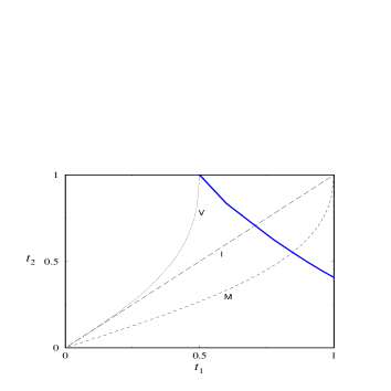
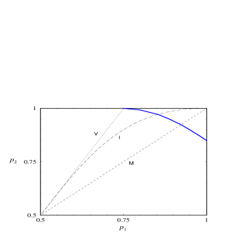
Figure 1: Phase diagram. Broken lines correspond to the noisy voter model (V), the Ising model (I) and the majority vote model (M). The low temperature phase is located in the upper right corner, above the transition line (full line).

Figure 1 shows, in the $(t_{1},t_{2})$ or $(p_{1},p_{2}$) planes, the lines corresponding to the Ising, voter and majority vote models. Three other lines deserve attention. Firstly, the $p_{2}=1$ line corresponds to models with no bulk noise ($T_{2}=0$), hence the dynamics is only driven by interfacial noise, defined above. Secondly, the $p_{1}=1$ line corresponds to models with no interfacial noise ($T_{1}=0$), hence the dynamics is only driven by bulk noise. (In both cases the effect due to the curvature of the interfaces is always present, as mentioned above.) For these last models, the local spin aligns in the direction of the majority of its neighbours with probability one, if the local field $h=2$, i.e. if there is no consensus amongst the neighbours. If there is consensus amongst them, i.e. if $h=4$, the local spin aligns with its neighbours with a probability $p_{2}<1$. Finally the transition line between the low and high temperature regions is discussed below.

See reference [16] for similar definitions. The introduction of the temperatures $T_{1}$ and $T_{2}$, together with their interpretations as given above, is original to the present work. A dual description of the dynamics of the models in terms of reaction diffusion processes is given in the appendix.

3 Phase ordering and the critical line

In this section we investigate the dynamics of phase ordering for the two parameter class of models presented here. For $p_{1}$ and $p_{2}$ given, we let the system evolve, starting from a random initial configuration. This study demonstrates the existence of a critical line, in the $(p_{1},p_{2})$ or $(t_{1},t_{2})$ planes, between a low temperature region where clusters (or domains) grow indefinitely, and a high temperature region where one only observes fluctuations at a finite scale. It also provides a visual illustration of the role of the two temperatures $T_{1}$ and $T_{2}$, respectively associated to interfacial and to bulk noise.

Two methods for updating the spins are at our disposal. With sequential updating, time is continuous and each spin evolve independently of others, at times chosen randomly according to a Poissonian law. The normalization is chosen such that each spin evolves once in a mean unit of time. Therefore, in a simulation of a lattice of $N$ spins, one has to choose randomly a spin and update it, $N$ times per time unit.

Instead of using sequential updating, we adopt a slightly different procedure for our simulations, namely a parallel updating of the spins. The lattice is divided into two odd and even sublattices, and, during a unit of time, the two sublattices are visited in turn, with a systematic update of their spins. This division is needed in order to avoid undesirable effects due to the simultaneous update of neighbouring sites. This process allows a functional parallelization on the computer. Spins are represented as single bits, and it is possible to arrange the spins into computer words, such that all spins of a word can be updated simultaneously by global logical operations. This method is numerically efficient, allowing for long simulations on large lattices.

In figures 2–7, we have selected snapshots of the same fragment $256\times 256$ of a $512\times 512$ lattice with periodic boundary conditions, for three times $t=8$, 64 and 512, and six different points in the parameter space of the models.

Figures 2, 3 depict, as reference views, the well known appearance of domain growth for the Ising model, respectively at zero temperature, and at $T=0.97\,T_{c}$. The Ising critical point corresponds to $t_{1}=t_{2}=1/\sqrt{2}$. For $T<T_{c}$ clusters grow as $\sqrt{t}$, while at $T_{c}$, they only grow as $t^{1/z}$, where the dynamical exponent $z\approx 2.17$. In the high temperature phase, clusters grow until their sizes reach the equilibrium correlation length.

Figure 2: Snapshots of the evolution for the Ising model at zero temperature ($p_{1}=p_{2}=1$).

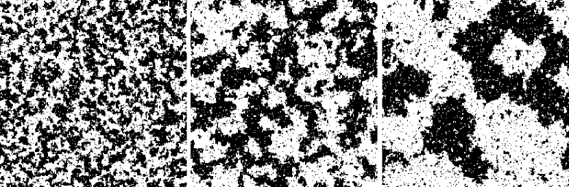
Figure 3: Snapshots of the evolution for the Ising model at $T=0.97\,T_{c}$ ($p_{1}=0.8602$, $p_{2}=0.9743$).

This distinction between a low temperature and a high temperature phase can be generalized to all models of the two dimensional parameter plane. The transition line between the low and high temperature regions, depicted in figure 1, was located by a systematic investigation of the parameter plane.

For instance, figures 4, 5, and 6 correspond to an exploration of the line $p_{2}=1$, with $p_{1}$ decreasing away from the zero temperature Ising case ($p_{1}=p_{2}=1$). On this line no thermal fluctuations occur inside the clusters, so their interiors remain forever uniformly black or white. When $p_{1}$ decreases, the boundaries between domains take progressively a fractal appearance, in accord with the fact that interfacial noise increases along the line. This is particularly visible on figure 4, which illustrates the case of a model close to the voter model, in the low temperature region ($p_{1}=0.76$, $p_{2}=1$), and on figure 5, for the voter model itself ($p_{1}=0.75$, $p_{2}=1$). Again one observes growing clusters, with a characteristic size behaving as $\sqrt{t}$. A similar behaviour is observed for all models such that $0.75\leq p_{1}\leq 1,p_{2}=1$.

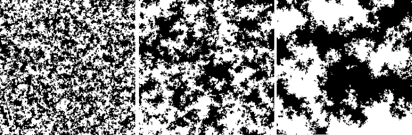
Figure 4: Snapshots of the evolution for a model close to the voter model, in the low temperature region ($p_{1}=0.76$, $p_{2}=1$).

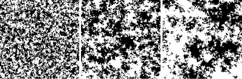
Figure 5: Snapshots of the evolution for the voter model ($p_{1}=0.75$, $p_{2}=1$).

Figure 6 illustrates the case of a model located in the high temperature region, near the voter model ($p_{1}=0.72$, $p_{2}=1$). In parallel to what is observed for the Ising case above $T_{c}$, clusters grow until their sizes reach the correlation length. The transition to the low temperature region along the line $p_{2}=1$ is therefore only induced by the interfacial noise.

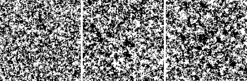
Figure 6: Snapshots of the evolution for a model close to the voter model, in the high temperature region ($p_{1}=0.72$, $p_{2}=1$).

We also display in figure 7 the evolution observed for the majority vote model with ($p_{1}=p_{2}=0.93$). The transition takes place for $p_{1}=p_{2}\approx 0.923$, in agreement with the value ($0.925$) given in [17].

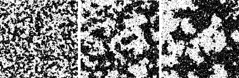
Figure 7: Snapshots of the evolution for the majority vote model ($p_{1}=p_{2}=0.93$).

Finally exploring the line $p_{1}=1$, we observe a transition between the low and high temperature regimes for $p_{2}\approx 0.849$, in agreement with the value ($0.854$) given in [16]. Figure 8 depicts snapshots of the evolution for the model with ($p_{1}=1$, $p_{2}=0.84$). See [16] for a determination of the critical line by a finite size scaling analysis in the stationary state.

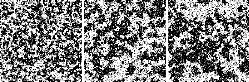
Figure 8: Snapshots of the evolution for the model with ($p_{1}=1$, $p_{2}=0.84$).

4 Persistence

In this section we address the question of persistence in the low temperature region of the ($p_{1},p_{2}$) parameter plane depicted in figure 1. We first present numerical measurements of the fraction $R(t)$ of spins which never flipped up to time $t$, for models with no bulk noise, i.e. for $T_{2}=0$ or $p_{2}=1$. The case of persistence at finite temperature, i.e. in the present context for $T_{2}>0$, will be discussed in section 4.2.

4.1 The $p_{2}=1$ line

We measured persistence in the low temperature region ($p_{1}\geq 0.75$) of the line $p_{2}=1$. Figure 9 depicts the results of simulations for times up to 5000, on a lattice $3072\times 3072$. The fraction $R(t)$ of spins which never flipped up to time $t$ behaves, in the early stage, as

$$\ln R(t)\sim-A\ln^{2}t+B\ln t+C+\cdots,$$ (17)

then one observes a crossover toward the power law

$$R(t)\sim t^{-\theta},$$ (18)

with an exponent $\theta\approx 0.22$ which seems independent of $p_{1}$. This behaviour therefore interpolates between the two ‘pure’ cases, namely the zero temperature Ising model ($p_{1}=p_{2}=1$) where (18) is observed with the same exponent $\theta\approx 0.22$ [7, 8, 9], and the voter model, for which (17) holds [10, 11].

Figure 9: Log-log plot of the persistence probability $R(t)$ on the line $p_{2}=1$, for $p_{1}=1,0.9,0.8,0.77,0.75$, from top to bottom. The inset depicts $\ln R(t)$ for the voter model ($p_{1}=0.75$) against $\ln^{2}t$. The system size is $L=3072$.

The origin of these two ‘pure’ behaviours can be simply traced back to the two driving forces of the dynamics in absence of bulk noise, i.e. respectively to interfacial noise for (17), and to the curvature of interfaces for (18). Indeed, consider first the case of the Ising model at zero temperature ($T_{1}=T_{2}=0$), for which the dynamics is only driven by the curvature of interfaces. As a consequence, the only flipping mechanism for a spin is the slow sweeping mode of the interfaces, hence persistent spins deeply buried inside large clusters disappear slowly, according to (18). Consider now the case of the voter model ($p_{1}=0.75,p_{2}=1$), starting from a configuration with a planar interface separating two regions of opposite spins. This interface thickens gradually, because of interfacial noise, taking ever more a fractal appearance. At large times it becomes difficult to speak any longer of an interface, the thickness of which should be considered as infinite. The decay of persistent spins is much faster and follows (17).

This analysis allows the following interpretation of the results given above for persistence of a generic model along the $p_{2}=1$ line, and $p_{1}>0.75$. In the early stages of coarsening, domains begin to grow and develop their interfaces. As a consequence, the fraction of persistent spins in the interface region is expected to decay more rapidly than if they were deep inside a cluster, following (17) since this is the dominant process. The duration of this early stage is related to the thickness of the interfaces, which vanishes for the Ising model where smooth interfaces are observed, and diverges for the voter model where a fractal appearance of the interfaces is observed. After this first stage, the fraction of persistent spins will decay according to (18). Therefore, along the line $p_{2}=1$ ($T_{2}=0$), the resulting law for the decay of $R(t)$ will be a weighted sum of (17) and (18). The amplitude obtained by fitting the asymptotic algebraic tail (18) is naturally interpreted as the fraction of persistent spins which are deep inside the clusters. This fraction vanishes when one approaches the voter model, with an apparent power law $(p_{1}-0.75)^{\alpha}$, with $\alpha\approx 2.3$. This result is consistent with the fact that the voter model is critical, according to the criterion of section 3.

Note that, for any model such that $p_{1}>0.75$, the prescription of suppressing the bulk noise by forbidding flips of a spin $\sigma=1$ (resp. $\sigma=-1$) surrounded by four spins with the same value $1$ (resp. $-1$), leads to an algebraic decay of the persistence probability. This corresponds to a projection of the model onto the line $p_{1}=1$.

4.2 Persistence at finite temperature

For a two dimensional Ising system in presence of thermal noise (i.e. in the present context, for $p_{2}<1$), the number of spins which did not flip up to time $t$ decays exponentially. A more satisfactory quantity to investigate is the fraction $R(t)$ of space which remained in the same phase, coming back to the original definition of persistence [18, 19], where ‘remaining in the same phase’ means remaining ‘dry’, i.e. unswept by an interface. The prescription given in [12] to determine whether a given spin ‘remained in the same phase’, leads again to algebraic decay of $R(t)$, the fraction of ‘persistent’ spins, when $T<T_{c}$. Further works [13, 14, 15] seem to indicate that the persistence exponent $\theta$ for the two dimensional Ising model is constant in the low temperature phase, and approximately equal to 0.22.

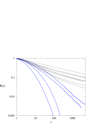
Figure 10: Log-log plot of the persistence probability $R(t)$. Full lines, from top to bottom: ($p_{1}=1,p_{2}=1$): Ising at $T=0$ ; ($p_{1}=0.95,p_{2}=0.997$): Ising at $T=0.6\,T_{c}$; ($p_{1}=1,p_{2}=0.95$); ($p_{1}=0.95,p_{2}=0.95$): Majority vote; ($p_{1}=0.9,p_{2}=1$); ($p_{1}=0.8,p_{2}=0.988$): Ising at $T=0.8\,T_{c}$; ($p_{1}=1,p_{2}=0.9$); ($p_{1}=0.876,p_{2}=0.980$): Ising at $T=0.9\,T_{c}$; Dashed lines, from top to bottom: ($p_{1}=0.92,p_{2}=0.92$): Majority vote; ($p_{1}=0.854,p_{2}=0.971$): Ising at $T=T_{c}$; ($p_{1}=1,p_{2}=0.84$); ($p_{1}=0.75,p_{2}=1$): Voter. The system size is $L=1536$.

Coming back to the class of models under investigation, one may therefore wonder what is the value of the persistence exponent outside the Ising line, in the low temperature region. Here we use the definition of [12], adopting the extensions given in [14], in order to measure persistence in the low temperature region of the parameter plane. We consider three copies of the system, A, B and C, submitted to the same noise ($p_{1},p_{2}$). The initial condition for A is random, while it is ordered for B ($\sigma_{i}^{\rm B}(0)=+1$), and C ($\sigma_{i}^{\rm C}(0)=-1$) where $i=1,\ldots,N$ labels the sites. A spin $\sigma_{i}^{\rm A}$ of copy A is said to be persistent up to time $t$, if it experienced thermal fluctuations only, i.e. if its history was either that of $\sigma_{i}^{\rm B}$ or that of $\sigma_{i}^{\rm C}$. Hence

$$R(t)=P\big{(}\sigma_{i}^{\rm A}(t^{\prime})=\sigma_{i}^{\rm B}(t^{\prime}),\ \text{or}\ \sigma_{i}^{\rm A}(t^{\prime})=\sigma_{i}^{\rm C}(t^{\prime}),\forall t^{\prime}\leq t\big{)}$$ (19)

measures the fraction of persistent spins in one of the two phases $\pm$ [14, 12]. We also checked, using the determination of the interfaces proposed in [14], the equivalence between the definition of $R(t)$ given by (19) and that obtained by considering a spin as persistent if it was not swept by an interface.

Figure 10 depicts the results. The exponent $\theta$ seems constant, with a value $\approx 0.22$, for all models on the low temperature side of the critical line that we considered. It is nevertheless hard to conclude, on the basis of numerical measurements. The decrease of persistence at criticality is much faster. A possible explanation is that, as for the voter model (see 4.1), the thickness of interfaces diverges, leading to a behaviour similar to (17).

5 Conclusion

The aim of the present work was to initiate the study of coarsening and persistence for a class of models interpolating between the voter and Ising models, introduced previously in [16].

In our opinion, the introduction of two temperatures $T_{1}$ and $T_{2}$, respectively associated to interfacial and bulk noise, gives a useful interpretation of the phenomena observed when varying continuously the parameters defining this class of models. The present analysis seems to indicate that $\theta\approx 0.22$ is the universal persistence exponent for all models in the low temperature phase. The situation on the critical line is less clear, and possibly related to the divergence of the interfaces between domains at criticality. In this respect it would be desirable to find a way of computing the equation of the critical line in the $(p_{1},p_{2})$ parameter plane. A more ambitious goal would be to compute $\theta$ for the two dimensional zero temperature Ising model, in the dual reaction diffusion framework given in the appendix, using the field theoretical methods of [20, 21, 22, 11]. Let us finally mention extensions to $d>2$ or to the Potts model as possible further studies. We hope to address some of those points in the future.

We wish to thank M Howard and J-M Luck for interesting discussions.

Appendix A The dual approach

In this appendix we show that the dynamics of this class of models possesses a dual description in terms of reaction diffusion processes for a set of random walkers moving backward in time. This description, beyond its intuitive value, is the starting point of an analysis of the temporal evolution of the system by means of diagrammatic expansions [23].

We first review the case of the voter model [3, 5, 6, 24]. Let us define the random variable $\tau=(1+\sigma)/2=1,0$, hereafter also called spin. The value of the spin $\tau^{(t)}_{x}$ at time $t$ and site $x$ can be traced back to the value of its ancestor $\tau_{y}^{(0)}$ at time $t=0$, located on site $y$. The idea is to follow the line of continuity of the value of the spin, backward in time, from ($x,t$) to ($y,0$). Indeed, one first follows the line of constant $\tau$ backward in time, from $(x,t)$ until the last updating of site $x$ is met. At this time, the spin had chosen the value of a neighbouring site. Moving to this site one again follows the line of constant $\tau$ backward in time. Proceeding until $t=0$, one thus performs a random walk, backward in time, from ($x,t$) to ($y,0$) such that $\tau_{x}^{(t)}=\tau_{y}^{(0)}$.

It is easy to see that all spins at time $t$ possess an ancestor at time $t=0$, but that conversely not all sites at time $t=0$ are ancestors of spins at time $t$. Indeed, starting from $n$ spins $\tau^{(t)}_{1},\ldots,\tau^{(t)}_{n}$, located on sites $x_{1},\ldots,x_{n}$, at time $t$, the same reasoning leads to the consideration of $n$ random walkers starting from sites $x_{1},\ldots,x_{n}$ at time $t$, and going backward in time. When two such walkers meet, they coalesce because the corresponding sites have a common ancestor from which they inherit the common value of their spin.

Figure 11: An example of coalescing random walks moving backward in time, occurring in the voter model. The drawing is done in one dimension, for simplicity.

Hence the determination of the values of these $n$ spins is equivalent, for the voter model, to knowing the history of $n$ independent coalescing random walkers, starting from sites $x_{1},\ldots,x_{n}$, and moving backward in time. An example is displayed in figure 11. The final stage, at time $t=0$, contains $k$ walkers ($1\leq k\leq n$) at sites $y_{1},\ldots,y_{k}$. Since $\tau_{x_{1}}^{(t)}\cdots\tau_{x_{n}}^{(t)}=\tau_{y_{1}}^{(0)}\cdots\tau_{y_{k}}^{(0)}$, we conclude that the sum of the probabilities of all these processes starting from the $n$ points $x_{1},\dots,x_{n}$ gives the correlation function $\langle\tau_{x_{1}}^{(t)}\cdots\tau_{x_{n}}^{(t)}\rangle$. One can easily generalize the reasoning to the case of spins on different sites $x_{1},\ldots,x_{n}$, at different times $t_{1},\ldots,t_{n}$.

For the voter model, the definition (9) can be rewritten as

$$P(\tau_{x}=1)=\frac{1}{4}\left(\tau_{y_{1}}+\tau_{y_{2}}+\tau_{y_{3}}+\tau_{y_{4}}\right).$$ (20)

This means that for a two dimensional random walk the elementary process consisting of a jump from site $x$ to one of its neighbouring sites $y$ has probability $\frac{1}{4}\tau_{y}$. Similarly (11) leads to

$$P(\tau_{x}=1)=1-p_{2}+(p_{2}-p_{1})\left(\tau_{y_{1}}+\tau_{y_{2}}+\tau_{y_{3}}+\tau_{y_{4}}\right),$$ (21)

the interpretation of which is given below. The generalization to a generic model ($p_{1},p_{2}$) is now straightforward. By its very definition one has

$$\begin{array}[]{l}P(\tau_{x}=1)=p_{2}\tau_{y_{1}}\tau_{y_{2}}\tau_{y_{3}}\tau_{y_{4}}\\ \quad+p_{1}\left[\tau_{y_{1}}\tau_{y_{2}}\tau_{y_{3}}\left(1-\tau_{y_{4}}\right)+\text{3perm.terms}\right]\\ \quad+\frac{1}{2}\left[\tau_{y_{1}}\tau_{y_{2}}\left(1-\tau_{y_{3}}\right)\left(1-\tau_{y_{4}}\right)+\text{5perm.terms}\right]\\ \quad+(1-p_{1})\left[\tau_{y_{1}}\left(1-\tau_{y_{2}}\right)\left(1-\tau_{y_{3}}\right)\left(1-\tau_{y_{4}}\right)+\text{3perm.terms}\right]\\ \quad+(1-p_{2})\left(1-\tau_{y_{1}}\right)\left(1-\tau_{y_{2}}\right)\left(1-\tau_{y_{3}}\right)\left(1-\tau_{y_{4}}\right)\end{array}$$ (22)

This expression can be rewritten as

$$\begin{array}[]{l}P(\tau_{x}=1)=1-p_{2}\\ \qquad+(p_{2}-p_{1})\left(\tau_{y_{1}}+\tau_{y_{2}}+\tau_{y_{3}}+\tau_{y_{4}}\right)\\ \qquad+\left(2p_{1}-p_{2}-\frac{1}{2}\right)\left(\tau_{y_{1}}\tau_{y_{2}}+\tau_{y_{1}}\tau_{y_{3}}+\tau_{y_{1}}\tau_{y_{4}}+\right.\\ \qquad\qquad\qquad\left.+\tau_{y_{2}}\tau_{y_{3}}+\tau_{y_{2}}\tau_{y_{4}}+\tau_{y_{3}}\tau_{y_{4}}\right)\\ \quad-\left(2p_{1}-p_{2}-\frac{1}{2}\right)\left(\tau_{y_{1}}\tau_{y_{2}}\tau_{y_{3}}+\tau_{y_{1}}\tau_{y_{2}}\tau_{y_{4}}+\tau_{y_{1}}\tau_{y_{3}}\tau_{y_{4}}+\tau_{y_{2}}\tau_{y_{3}}\tau_{y_{4}}\right)\end{array}$$ (23)

Equation (23) is the generalization of (21) and can be expressed as the sum of four elementary processes, namely:

• the random walker disappears (with a weight $1-p_{2}$),

• the random walker makes a step to a neighbouring site (with a weight $p_{2}-p_{1}$),

• the random walker splits into two walkers located on different neighbouring sites (with a weight $2p_{1}-p_{2}-\frac{1}{2}$),

• the random walker splits into three walkers located on different neighbouring sites (with a weight $-2p_{1}+p_{2}+\frac{1}{2}$).

Hence the coalescing random walks considered above for the voter model have now also the possibility of annihilating, or of branching into two or three new walks. Note that the weight $p_{2}-p_{1}$ vanishes on the line of the majority vote model, while the weight $2p_{1}-p_{2}-\frac{1}{2}$ vanishes on the line of the noisy voter model.

Let us underline the fact that the weights corresponding to these elementary processes can be negative. Therefore these drawings should be seen as diagrams, and not as the actual paths of real random walkers. They may indeed be used for actual diagrammatic computations. For example, near the voter model, one can perform a double series expansion of the correlation functions in the ‘coupling constants’ $1-p_{2}$ and $2p_{1}-p_{2}-\frac{1}{2}$, in order to compute the rate of the exponential decay of persistence, in good agreement with numerical measurements [23].

References

References

- [1] Langer J S 1991 in Solids far from equilibrium Godrèche C ed (Cambridge University Press)
- [2] Bray A J 1994 Adv. Phys. 43 357
- [3] Liggett T M 1985 Interacting Particle Systems (Springer Verlag)
- [4] Glauber R J 1963 J. Math. Phys. 4 294
- [5] Cox J T and Griffeath D 1986 Ann. Probab. 14 347
- [6] Scheucher M and Spohn H 1988 J. Stat. Phys. 53 279
- [7] Derrida B, Bray A J and Godrèche C 1994 \JPA27 L357
- [8] Stauffer D 1994 \JPA27 5029
- [9] Derrida B, de Oliveira P M C and Stauffer D 1996 Physica A 224 604
- [10] Ben-Naim E, Frachebourg L and Krapivsky P L 1996 \PRE 53 3078
- [11] Howard M and Godrèche C 1998 J. Phys. A: Math. Gen. 31 L209
- [12] Derrida B 1997 Phys. Rev. E 55 3705
- [13] Stauffer D 1997 Int. J. Mod. Phys. C 8 361
- [14] Hinrichsen H and Antoni M 1998 cond-mat/9710263
- [15] Cueille S and Sire C 1997J. Phys. A: Math. Gen. 30 L791; 1998 cond-mat/9803014
- [16] de Oliveira M J, Mendes J F F and Santos M A 1993 J. Phys. A: Math. Gen. 26 2317
- [17] de Oliveira M J 1992 J. Stat. Phys. 66 273
- [18] Marcos-Martin M, Beysens D, Bouchaud J-P, Godrèche C and Yekutieli I 1995 Physica A 214 396
- [19] Bray A J, Derrida B and Godrèche C 1994 Europhys. Lett. 27 175
- [20] Lee B P 1994 J. Phys. A: Math. Gen. 27 2633
- [21] Howard M and Cardy J 1995 J. Phys. A: Math. Gen. 28 3599
- [22] Cardy J 1995 J. Phys. A: Math. Gen. 28 L19
- [23] Drouffe J-M and Godrèche C unpublished
- [24] Derrida B 1995 J. Phys. A: Math. Gen. 28 1481