Anomalous Mesoscopic Fluctuations of Transport Coefficients Above The Critical Temperature

Abstract

We show in this paper that above the critical temperature of superconductor-metal phase transitions, both the longitudinal and Hall conductivity exhibit strong temperature dependent mesoscopic fluctuations, with amplitudes much larger than the mesoscopic fluctuations in noninteracting normal metals. Such an enhancement of the mesoscopic fluctuations arises from pairing correlations and is strongly dependent on dimensions.

It is well known that the conductance of a normal metal exhibits mesoscopic fluctuations if the sample size $L$ is smaller than the dephasing length $L_{\phi}$^[1,2,3]. At zero temperature, the amplitude of the mesoscopic fluctuations is of order $e^{2}/\hbar$, independent of the dimensionality of the sample. These mesoscopic fluctuations originate from quantum interference of electrons and are sensitive to changes in external magnetic fields, impurity configurations, or gate voltages.

Universal conductance fluctuations(UCF), of order $e^{2}/\hbar$, are closely connected with the universality of Wigner-Dyson statistics of single electron levels in disordered metals. For a normal metal, the conductance is equal to $e^{2}/\hbar$ times $N$, the number of single electron levels inside an energy band of the width of the Thouless energy $E_{T}$ centered at the Fermi surface. The Thouless energy is the inverse of the time required for an electron to diffuse across the sample^[4]. While the average number of levels within such an energy band depends on the dimensionality, $\delta N$, the fluctuation of the number of single electron levels within such a band is universally of order of 1^[5]. This leads to UCF.

At finite temperature, the transport currents are carried by the quasi particle excitations of energy of order $kT$. While the total number of electron levels involved is $NT/E_{T}$, the amplitude of the fluctuation of the number of levels is $(L/L_{T})^{d/2}=(T/E_{T})^{d/4}$, due to the fact that the mesoscopic fluctuations of the density of states are correlated at a length scale $L_{T}\ll L$ and the contributions from different blocks should be summed up randomly^[5]. Here $L_{T}=\sqrt{D/T}$ is the normal metal coherence length at temperature $T$, $D$ is the diffusion constant. The relative amplitude of the fluctuation of number of levels decreases as the temperature is increased. Therefore the amplitude of the conductance fluctuation is smaller than $e^{2}/\hbar$ when the temperature is higher than $E_{T}$^[5].

The above statement about mesoscopic fluctuations of the conductance remains true in weakly correlated electron systems. For instance, the electron-electron interaction in normal metals barely affect universal conductance fluctuations. For strongly correlated systems, could be fractional quantum Hall systems, or quantum dots in the Coulomb blockade regime, the amplitude of the conductance fluctuation is also of the order of or less than $e^{2}/\hbar$.

In this paper we study the effect of pairing correlations on the mesoscopic fluctuations of the conductance. We show that above the critical temperature, in the presence of pairing correlations, mesoscopic fluctuations of conductance can greatly exceed $e^{2}/\hbar$, that of UCF. Such an effect increases when the critical temperature is approached. It also strongly depends on dimensionalities of samples, originating from the fact that pairing correlations due to thermal fluctuations strongly depend on dimensionalities.

The qualitative mechanism for this phenomenon is as follows. Above $T_{c}$ the critical temperature of superconductor-metal phase transitions, there is a finite amplitude for electrons to form superconducting pairs with a certain relaxation time. Thus transport coefficients in normal metals can be written as a sum of classical Drude conductivities and contributions arising from pairing correlations. The amplitude of thermal fluctuations of superconducting pairs are determined by a competition between the entropy and the condensation energy and becomes divergent when the temperature approaches $T_{c}$ from above. The typical relaxation time is given as the time scale for pairs to diffuse over the Landau-Ginsburg length scale and is also divergent when the critical temperature is approached. As a result, the conductivity is enhanced via

$$\frac{\delta\sigma}{\sigma}\propto\int\frac{d{\bf Q}^{d}}{(2\pi)^{d}}\Delta_{\bf Q}\Delta_{\bf Q}\tau_{\bf Q}=\frac{1}{g_{d}}\left(\frac{T}{T-T_{c}}\right)^{(4-d)/2}$$ (1)

$$\Delta_{\bf Q}\Delta_{\bf Q}=\nu^{-1}\left(\frac{T-T_{c}}{T}+\frac{D{\bf Q}^{2}}{T}\right)^{-1},\tau_{\bf Q}=\frac{1}{D{\bf Q}^{2}+T-T_{c}}.$$ (2)

where $\nu$ is the density of states in normal metals; $g_{d}$ is the dimensionless conductance of the size of $L_{T}$, and $d$ is the dimensionality. The dimensionless conductance in each dimension is $g_{3}=2\pi^{2}\hbar\sigma L_{T}/e^{2}$, $g_{2}=4\pi\hbar\sigma t/e^{2}$ and $g_{1}=6\pi\hbar\sigma a^{2}/L_{T}e^{2}$, $t$ is the film thickness in $2D$, $a$ is the diameter in $1D$. $\sigma=e^{2}\nu D$ is the Drude conductivity. Integral $\int d{\bf Q}^{d}/(2\pi)^{d}$ is $\int d{\bf Q}^{3}/(2\pi)^{3}$ in $3D$, $1/t\int d{\bf Q}^{2}/(2\pi)^{2}$ in $2D$ and $1/a^{2}\int d{\bf Q}/(2\pi)$ in $1D$. Eq.1 is valid as far as the correction is small .i.e., $\delta\sigma/\sigma\ll 1$.

However, the condensation energy has mesoscopic fluctuations, as emphasised in Ref. 6. The fluctuation amplitude is $1/g_{d}$ and its correlation length is min$\{L_{T},\xi_{0}\}$. Here $\xi_{0}=\sqrt{\hbar D/T_{c}}$ is the coherence length of superconductors at zero temperature. This effectively leads to mesoscopic fluctuations of the critical temperature, ${\delta T_{c}}/{T_{c}}\propto g_{d}^{-1}({\xi_{0}}/{L})^{4-d/2}$ where we take into account that $L\gg\xi_{0}$ and fluctuations from different blocks of the size of $\xi_{0}$ should be summed up randomly. Therefore the pairing amplitude calculated in Eq.1 develops giant mesoscopic fluctuations $\delta\Delta^{M}_{\bf Q}\delta\Delta^{M}_{\bf Q}$ near the critical point,

$$\frac{\delta\Delta^{M}_{\bf Q}\delta\Delta^{M}_{\bf Q}}{\Delta_{\bf Q}\Delta_{\bf Q}}\propto\left(\frac{1}{g_{d}}\right)\left(\frac{\xi_{0}}{L}\right)^{4-d/2}\left(\frac{T}{T-T_{c}+D{\bf Q}^{2}}\right).$$ (3)

Substituting Eq.2 into $\delta\sigma$ in Eq. 1 we obtain an estimate of mesoscopic fluctuations of the conductance, of the same order as that given in Eq.8. Mesoscopic fluctuations of the conductance in this regime are therefore determined by mesoscopic fluctuations of pairing correlations. This results in anomalous mesoscopic fluctuations of transport coefficients in such systems.

To proceed further, we express the conductivity of a given sample above $T_{c}$ as $\sigma_{xx}=\sigma+\delta\sigma+\delta\sigma^{M}_{xx}$. $\delta\sigma$ represents the contributions from Aslamazov-Larkin and Maki Thompson corrections due to thermal fluctuations, studied in Refs. 7.8. It is divergent as the temperature approaches $T_{c}$, as shown in Eq.1. The mesoscopic fluctuations of the conductivity $\delta\sigma^{M}_{xx}$ as a function of gate voltage $V_{g}$ are given in terms of diagrams in Fig.a),

$$<\delta\sigma^{M}_{xx}(V_{g1})\delta\sigma^{M}_{xx}(V_{g2})>=<\delta\sigma^{M}_{AL}(V_{g1})\delta\sigma^{M}_{AL}(V_{g2})>+<\delta\sigma^{M}_{MT}(V_{g1})\delta\sigma^{M}_{MT}(V_{g2})>,$$ (4)

(5)

$$<\delta\sigma^{M}_{AL}(V_{g1})\delta\sigma^{M}_{AL}(V_{g2})>=\left(\frac{4e^{2}}{\hbar\pi}\right)^{2}\left(\frac{\pi D}{8T_{c}}\right)^{4}\int\frac{d{\bf Q_{1}}^{d}}{(2\pi)^{d}}\frac{d{\bf Q_{2}}^{d}}{(2\pi)^{d}}{\bf Q_{1}}^{2}{\bf Q_{2}}^{2}\int^{+\infty}_{-\infty}d\omega_{1}d\omega_{2}\coth\left(\frac{\omega_{1}}{2T}\right)\coth\left(\frac{\omega_{2}}{2T}\right)$$ (6)

$$\frac{\partial^{2}}{\partial\omega_{1}\partial\omega_{2}}\left\{ImL^{R}(\omega_{1},{\bf Q_{1}}^{2})ImL^{R}(\omega_{2},{\bf Q_{2}}^{2})<Im\delta L^{R}(\omega_{1},{\bf Q}_{1}^{2})Im\delta L^{R}(\omega_{2},{\bf Q}_{2}^{2})>\right\},$$ (7)

(8)

$$<\delta\sigma^{M}_{MT}(V_{g1})\delta\sigma^{M}_{MT}(V_{g2})>=\left(\frac{4e^{2}}{\hbar\pi}\right)^{2}D^{2}\int\frac{d{\bf Q_{1}}^{d}}{(2\pi)^{d}}\frac{d{\bf Q_{2}}^{d}}{(2\pi)^{d}}{\cal C}_{0}({\bf Q_{1}}^{2}){\cal C}_{0}({\bf Q_{2}}^{2})\int_{0}^{\infty}d\omega_{1}d\omega_{2}\coth\left(\frac{\omega_{1}}{2T}\right)\coth\left(\frac{\omega_{2}}{2T}\right)$$ (9)

$$\frac{\partial^{2}}{\partial\omega_{1}\partial\omega_{2}}\left\{Im\Psi\left(\frac{1}{2}+\frac{i\omega_{1}}{4\pi T}\right)Im\Psi\left(\frac{1}{2}+\frac{i\omega_{2}}{4\pi T}\right)<Im\delta L^{R}(\omega_{1},{\bf Q_{1}}^{2})Im\delta L^{R}(\omega_{2},{\bf Q_{2}}^{2})>\right\}.$$ (10)

Here the lowercase $AL$ and $MT$ represent mesoscopic fluctuations of Aslamazov-Larkin and Maki-Thompson corrections to the conductivity respectively. We neglect mesoscopic fluctuations of conductivities associated with normal quasi-particles as the temperature is close to $T_{c}$ . $<...>$ denotes the average over impurity scattering potentials. $\Psi$ is the digamma function. $Im\delta L^{R}=(\delta L^{R}-\delta L^{A})/2i$. The propagators $L^{R,A}$, $\delta L^{R,A}$ are defined as

$$L^{R,A}(\omega,{\bf Q}^{2})=\left(\frac{T-T_{c}}{T}+\frac{\pi}{8}\frac{D{\bf Q}^{2}\pm i\omega}{T}+\frac{\omega}{2}\frac{\partial\ln T_{c}}{\partial\epsilon_{F}}\right)^{-1}$$ (11)

$$\delta L^{R,A}(\omega,{\bf Q}^{2})=L^{R,A}(\omega,{\bf Q}^{2})^{2}\int d\epsilon\tanh(\frac{\epsilon}{2kT})$$ (12)

$$\frac{1}{\nu V}\int d{\bf r}d{\bf r}^{\prime}\exp(i{\bf Q}\cdot({\bf r}-{\bf r}^{\prime}))\left\{G^{R}_{\epsilon+\omega}({\bf r},{\bf r}^{\prime})G^{A}_{-\epsilon}({\bf r},{\bf r}^{\prime})-<G^{R}_{\epsilon+\omega}({\bf r},{\bf r}^{\prime})G^{A}_{-\epsilon}({\bf r},{\bf r}^{\prime})>\right\},$$ (13)

where $V$ is the volumn of the sample. $G^{R,A}$ are the exact retarded and advanced Green function in the presence of disorder. $\delta L^{R,A}(\omega_{1},{\bf Q}_{1}^{2})$, $\delta L^{R,A}(\omega_{2},{\bf Q}_{2}^{2})$ are evaluated in the presence of gate voltages $V_{g1}$ and $V_{g2}$ respectively. $<\delta L^{R,A}>=0$ and the correlation function is given as

$${<\delta L^{R,A}(\omega_{1},{\bf Q}_{1}^{2})\delta L^{R,A}(\omega_{2},{\bf Q}_{2}^{2})>}=L^{R,A}(\omega_{1},{\bf Q}_{1}^{2})^{2}L^{R,A}(\omega_{2},{\bf Q}_{2}^{2})^{2}$$ (14)

$$\int_{-\infty}^{+\infty}d\epsilon d\epsilon^{\prime}\frac{1}{2\epsilon}\frac{1}{2\epsilon^{\prime}}\tanh(\frac{\epsilon}{2T})\tanh(\frac{\epsilon^{\prime}}{2T})\frac{1}{\nu^{2}V^{2}}\int d{\bf r}d{\bf r}^{\prime}\{Re{\cal C}^{2}_{\epsilon-\epsilon^{\prime}}({\bf r},{\bf r^{\prime}})+Re{\cal D}^{2}_{\epsilon-\epsilon^{\prime}}({\bf r},{\bf r^{\prime}})\}$$ (15)

in the leading order of $T-T_{c}/T_{c}$. ${\cal D}_{\epsilon-\epsilon^{\prime}}({\bf r},{\bf r^{\prime}})=\nu^{-1}<G^{R}_{\epsilon}({\bf r},{\bf r^{\prime}})G^{A}_{\epsilon^{\prime}}({\bf r}^{\prime},{\bf r})>$, ${\cal C}_{\epsilon-\epsilon^{\prime}}({\bf r},{\bf r^{\prime}})=\nu^{-1}<G^{R}_{\epsilon}({\bf r},{\bf r^{\prime}})G^{A}_{\epsilon^{\prime}}({\bf r},{\bf r}^{\prime})>$, are the diffusons and cooperons. Generally, they satisfy

$$\{i\omega+ie\phi_{1}({\bf r})-ie\phi_{2}({\bf r})+D(i\hbar\nabla-\frac{e}{c}{\bf A}_{1}({\bf r})\pm\frac{e}{c}{\bf A}_{2}({\bf r}))^{2}\}{\cal D}({\cal C})_{\omega}({\bf r},{\bf r}^{\prime})=\delta({\bf r}-{\bf r^{\prime}})$$ (16)

and ${\cal D}={\cal C}=0$ at the boundary for open geometry samples^[1,2]. $\phi_{1(2)}$ is the electrical potential induced via the gate voltage $V_{g1(2)}$ and ${\bf A}_{1(2)}$ is the vector potential in the presence of a magnetic field. ${\cal C}_{0}({\bf Q}^{2})$ in Eq.3 is the Fourier transformation of ${\cal C}_{0}({\bf r},{\bf r}^{\prime})$. The last term in the expression of $L^{R,A}$ in Eq.4 is from the dependence of the Fermi energy, $\epsilon_{F}$, of the critical temperature, $T_{c}$, and is inversely proportional to $\epsilon_{F}$. It is important only when the Hall conductivity is concerned^[9,10].

At $V_{g1}=V_{g2}$ in the absence of magnetic fields, Eq.5 yields

$$<\delta L^{R,A}(\omega_{1},{\bf Q}_{1}^{2})\delta L^{R,A}(\omega_{2},{\bf Q}_{2}^{2})>=L^{R,A}(\omega_{1},{\bf Q}_{1}^{2})^{2}L^{R,A}(\omega_{2},{\bf Q}_{2}^{2})^{2}\frac{\alpha_{d}}{g_{d}^{2}}\left(\frac{L_{T}}{L}\right)^{4-d}.$$ (17)

Here $\alpha_{d}$ are the constants dependent on the geometry and the dimensionality of the sample. When $\xi(T)=\sqrt{D/(T-T_{c})}\gg L$, in the open geometry in which we are interested, the most divergent contribution to the Aslamazov-Larkin and the Maki Thompson corrections to the conductivity is determined by the fluctuations with ${\bf Q}=\pi/L$, i.e, $L^{R}(\omega,{\bf Q}=\pi/L)$. Substituting Eq.7 into Eq.3, we obtain the amplitude of mesoscopic fluctuations of the conductivity above the critical temperature

$$\frac{<(\delta\sigma_{xx}^{M})^{2}>}{\sigma^{2}}=\frac{\beta_{d}}{g^{4}_{d}}\left(\frac{T}{T-T_{c}}\right)^{\frac{8-d}{2}}\left(\frac{\xi(T)}{L}\right)^{4-d},$$ (18)

when $L\gg\xi(T)$ and saturates as

$$\frac{<(\delta\sigma_{xx}^{M})^{2}>}{\sigma^{2}}=\frac{\beta_{d}}{g^{4}_{d}}\left(\frac{T}{E_{T}}\right)^{\frac{8-d}{2}},$$ (19)

when $L\ll\xi(T)$. Here $\beta_{3}\propto 1$, $\beta_{2}\propto max\{\ln(L/\xi(T)),1\}$ and $\beta_{1}\propto max\{L/\xi(T),1\}$. We want to emphasize that the mesoscopic fluctuations discussed here strongly depend on the dimensionality of a sample, which is in contrast to the theory of $UCF$. This is a direct consequence of mesoscopic fluctuations of pairing correlations.

Eqs.8, 9 are valid as far as $\delta\sigma^{M}_{xx}\ll\delta\sigma\ll\sigma$. Following Eqs.8,9, mesoscopic fluctuations of conductances can be much larger than $e^{2}/\hbar$. For instance, for a $2D$ film of the size of $\xi(T)$, at the temperature $T-T_{c}\sim T_{c}/g_{2}$ when $\delta\sigma/\sigma\sim 1$,

$$\sqrt{<(\delta\sigma_{xx}^{M})^{2}>}\propto\frac{e^{2}}{t\hbar}\sqrt{g_{2}}$$ (20)

is parametrically larger than UCF in normal metals.

The anomalous fluctuations can be probed in experiments where resistances are measured at different gate voltages. Let us consider a $2D$ film where a gate voltage is applied to the top of the film with capacitance $C$. The electric field induced by the gate is normal to the film and is screened over a Debye screening length $r_{0}=(e^{2}\nu)^{-1/2}$. Substituting Eqs. 5, 6 at ${\bf A}_{1}={\bf A}_{2}=0$ into Eq.3, we obtain the gate voltage dependence of the mesoscopic fluctuations

$${<(\delta\sigma_{xx}^{M}(V_{g1})-\delta\sigma^{M}_{xx}(V_{g2}))^{2}>}=<(\delta\sigma_{xx}^{M})^{2}>F(\frac{|V_{g1}-V_{g2}|Cr^{2}_{0}}{\epsilon_{0}tL^{2}T})$$ (21)

where

$$F(x)\propto\left\{\begin{array}[]{cc}x,&\mbox{$x\ll 1$}\\ 1,&\mbox{$x\gg 1$}\end{array}\right.$$ (23)

Following Eq.11, in this case, the characteristic gate voltage $V_{g}$ at which $\delta\sigma^{M}_{xx}(V_{g})$ are correlated is $\epsilon_{0}TL^{2}t/er^{2}_{0}C$. Mesoscopic fluctuations discussed here are also sensitive to external magnetic fields. At $E_{T}={D/L^{2}}\ll DH\ll T-T_{c}$, we can neglecte the magnetic field dependence of $L^{R,A}$ in the leading order of $DH/(T-T_{c})$. As a result, the correlation of conductance fluctuations as a function of magnetic field is determined by Eq.3, with $<Im\delta L^{R}(V_{g1})Im\delta L^{R}(V_{g2})>$ replaced with $<Im\delta L^{R}({\bf H})Im\delta L^{R}(0)>$. Taking into account Eqs.5,6 at $\phi_{1}=\phi_{2}$, we obtain conductance fluctuations of a 2D film as functions of a magnetic field ${\bf H}$ perpendicular to the film

$$\frac{<(\delta\sigma_{xx}^{M}({\bf H})-\delta\sigma^{M}_{xx}(0))^{2}>}{<\delta\sigma_{xx}^{M}\delta\sigma_{xx}^{M}>}\propto\frac{DH}{T}.$$ (24)

Eq. 13 is valid when $E_{T}\ll DH\ll T-T_{c}$ and saturates when $DH\gg T-T_{c}$. Eq. 13 shows that $\sigma(H)$ diffuses in $H$ space, with diffusion constant $<(\delta\sigma_{xx}^{M})^{2}>L_{T}^{2}/\Phi_{0}$, and the mean free time $\Phi_{0}L^{-2}$, $\Phi_{0}=\hbar c/e$ is the flux quantum. However, the average pairing correlation is also suppressed in the presence of external fields^[7,8,9,10], with the characteristic magnetic field corresponding to one flux per area of the size $\xi^{2}(T)$. Thus, in conductivity measurements, the dependence of mesoscopic fluctuations on magnetic fields should be differentiated from the average magnetoresistance. The other possibility to observe the anomalous mesoscopic fluctuations of transport coefficients is to measure the conductance during different thermal cycles.

Let us now turn to mesoscopic fluctuations of the Hall conductivity. Again one can write for a given sample, $\sigma_{xy}=\tau\Omega_{c}\sigma+\delta\sigma_{xy}+\delta\sigma^{M}_{xy}$. The first term is the Hall conductivity obtained from the classical Boltzmann transport equation, where $\Omega_{c}=eH/mc$ is the cyclotron frequency. The second term is the correction to the classical result due to pairing correlations above $T_{c}$, $\delta\sigma_{xy}\propto\tau\Omega_{c}\sigma/g_{d}(T/T-T_{c})^{(6-d)/2}$ as calculated in Ref.9, 10. $\delta\sigma^{M}_{xy}$ represents mesoscopic fluctuations of the Hall conductivity. The propagator in the presence of an external magnetic field is determined by diagrams in Fig.b),

$$L^{R}(\omega,{\bf Q})\frac{D{e{\bf A}_{H}\cdot{\bf Q}}}{T}L^{R}(\omega,{\bf Q})$$ (25)

proportional to ${\bf A}_{H}\cdot{\bf Q}$. This leads to one more $L^{R}(\omega,{\bf Q})$ in the expression for Hall conductivity than in Eq.3 and yields a more divergent temperature dependence of $\delta\sigma^{M}_{xy}$ as $T_{c}$ is approached. Here ${\bf A}_{H}$ is the vector potential of the external magnetic field ${\bf H}={\bf q}\times{\bf A}_{H}$, ${\bf E}$ is the electrical field. Noticing that ${\bf A}_{H}\cdot{\bf Q}{\bf E}\cdot{\bf q}{\bf Q}={\bf Q}^{2}{\bf E}\times{\bf H}$, taking into account the gradient of $T_{c}$ at the Fermi surface in the fluctuation propagtors, as shown in Eq.4, in the leading order of $T_{c}/\epsilon_{F}$, we obtain mesoscopic fluctuations of the Hall conductivity,

$$<(\delta\sigma^{M}_{xy})^{2}>=(\tau\Omega_{c})^{2}\frac{e^{4}}{\hbar^{2}}\left(\frac{\pi D}{8T^{2}}\right)^{4}\int\frac{d{\bf Q_{1}}^{d}}{(2\pi)^{d}}\frac{d{\bf Q_{2}}^{d}}{(2\pi)^{d}}{\bf Q_{1}}^{2}{\bf Q_{2}}^{2}\int_{-\infty}^{+\infty}d\omega_{1}d\omega_{2}\frac{\omega_{1}\omega_{2}}{\sinh^{2}\left(\frac{\omega_{1}}{2T}\right)\sinh^{2}\left(\frac{\omega_{2}}{2T}\right)}$$ (26)

$$((ImL^{R}(\omega_{1},{\bf Q}_{1}^{2}))^{3}(ImL^{R}(\omega_{2},{\bf Q}_{2}^{2}))^{3}<Re\delta L^{R}(\omega_{1},{\bf Q}_{1}^{2})Re\delta L^{R}(\omega_{2},{\bf Q}_{2}^{2})>+9(ImL^{R}(\omega_{1},{\bf Q}_{1}^{2}))^{2}$$ (27)

$$\times(ImL^{R}(\omega_{2},{\bf Q}_{2}^{2}))^{2}ReL^{R}(\omega_{1},{\bf Q}_{1}^{2})ReL^{R}(\omega_{2},{\bf Q}_{2}^{2})<Im\delta L^{R}(\omega_{1},{\bf Q}_{1}^{2})Im\delta L^{R}(\omega_{2},{\bf Q}_{2}^{2})>).$$ (28)

We neglect the Maki-Thompson contribution to the Hall conductivity because it is less divergent than the result in Eq.15.

Substituting Eq.5 into Eq.15, we obtain

$$\frac{<(\delta\sigma_{xy}^{M})^{2}>}{\sigma^{2}}=(\tau\Omega_{c})^{2}\frac{\gamma_{d}}{g^{4}_{d}}\left(\frac{T}{T-T_{c}}\right)^{\frac{12-d}{2}}\left(\frac{\xi(T)}{L}\right)^{4-d},$$ (29)

when $L\gg\xi(T)$; When $L\ll\xi(T)$,

$$\frac{<(\delta\sigma_{xy}^{M})^{2}>}{\sigma^{2}}=(\tau\Omega_{c})^{2}\frac{\gamma_{d}}{g^{4}_{d}}\left(\frac{T}{E_{T}}\right)^{\frac{12-d}{2}}.$$ (30)

Here $\gamma_{d}$ is a constant of order of unity, dependent on dimensionalities of samples. Eqs. 16, 17 are valid when $\delta\sigma_{xy}\ll\tau\Omega_{c}\sigma$, i.e. $T-T_{c}\gg T_{c}/g^{2/(6-d)}_{d}$. For a $2D$ sample of the size of order of $\xi(T)$, at the temperature $T-T_{c}\sim T_{c}/g^{1/2}_{2}$,

$$\sqrt{<(\delta\sigma_{xy}^{M})^{2}>}\propto\tau\Omega_{c}\frac{e^{2}}{t\hbar}g_{2}^{\frac{1}{4}}.$$ (31)

Generally speaking, in a disordered mesoscopic sample, mesoscopic fluctuations of the transverse conductivity are nonzero even in the absence of an external magnetic field^[3]. However, as usual, by reversing directions of external magnetic fields, one can measure the Hall conductivity and its mesoscopic fluctuations as the asymmetrical part of $\sigma_{xy}({\bf H})$.

In conclusion, we would like to point out that in a few recent experiments, giant mesoscopic fluctuations of conductance have been found in granular superconductors above their critical temperatures^[11,12]. We believe that the mechanism discussed in this paper is relevant for those phenomena. At zero temperature, it was shown that mesoscopic fluctuations of the condensation energy could lead to a superconducting glass state^[6]. F. Zhou would like to thank Aviad Frydman for sending him the preprint of his group’s work and Y. Liu for showing him unpublished data. We acknowledge illuminating discussions with B. Altshuler, B. Spivak, A. A. Varlamov. F. Zhou is supported by Princeton University. C. Biagini is supported in part under PRA97-QTMD in Italy. We also like to thank NEC research Institute for its hospitality.

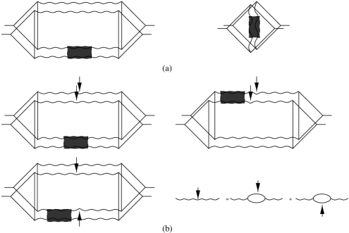
FIG. 1.: Diagrams for anomalous mesoscopic fluctuations of transport coefficients above the critical temperature. In a), b), the solid lines represent electron Green functions, the wave lines represent propagator $L^{R,A}$; the wave lines with shaded boxes represent $<\delta L^{R,A}\delta L^{R,A}>$, given in Eq.5. In b), the wave lines carrying arrows represent the propagators in the presence of magnetic fields. Triangles stand for current vertices and external electrical field vertices.

REFERENCES

• [1] P. A. Lee, A. D. Stone, Phys. Rev. Lett. 55, 1622
• [2] B. I. Altshuler, Pisma Zh. Eksp. Teor. Fiz. 42, 530 [JETP Lett. 41, 648(1985)].
• [3] it Mesoscopic Phenomena in Solids, edited by B. Altshuler, P. Lee, R. Webb, Elsevier Science Publishers B. V., 1991.
• [4] D. Thouless, Phys. Rev. Lett. 39, 1167(1977)
• [5] B. L. Altshuler, B. I. Shklovskii, Zh. Eksp. Teor. Fiz. 91, 220[ Sov. Phys. JETP 64, 127]
• [6] B. Spivak, F. Zhou, Phys. Rev. Lett. 74, 2800(1995); F. Zhou, B. Spivak, to appear in Phys. Rev. Lett., 1998.
• [7] L. G. Aslamasov, A. I. Larkin, Fiz. Tverd. Tela, 10, 1104(1968)[Sov. Phys. Solid. State 10, 975(1968)].
• [8] K. Maki, Prog. Theor. Phys. 39, 387(1968). R. S. Thompson, Phys. Rev. B 1, 327(1970).
• [9] H. Fukuyama, H. Ebisawa, T. Tsuzuki, Prog. Theor. Phys. 46, 1028(1971).
• [10] A. G. Aronov, S. Hikami, A.I. Larkin, Phys. Rev. B 51, 3880(1995).
• [11] A. Frydman, E. P. Price, R. C. Dynes, preprint, 1998.
• [12] Y. Liu, unpublished.
Refer to caption