Enhancement of coherent light amplification
using Anderson localization

Abstract

Several aspects of interplay between Anderson localization and coherent amplification/absorption, and aspect of mirrorless laser for a laser-active (amplifying) disordered dielectric medium have been addressed. We have calculated the statistics of the reflection coefficient and the associated phase for a light wave reflected from a coherently amplifying/absorbing one-dimensional disordered dielectric medium for different lengths, different disorder strengths and different ”amplification”/”absorption” parameters of the disordered sample. Problems with modeling coherent amplification/absorption by complex potential have been discussed. We have shown an alternative way to model the coherent absorption. Several conceptual and physical aspect for coherently amplifying/absorbing media with disorder also have been discussed.

I introduction

Wave propagation in disordered media and its consequences to the disorder induced localization, or Anderson localization [2] have been studied in detail for electron (quantum) waves [3], as well as for light (classical) waves [4] for last four decades. We have discussed several aspects of transport and localization for 1D electronic systems in our previous paper [5]. In this paper we are dealing with an interesting aspect of the application of the Anderson localization to enhance the coherent light amplification in a coherently amplifying disordered medium. Due to the bosonic nature of the light quanta, there is possibility of coherent amplification or coherent absorption(attenuation) for light; and these possibilities are absent for electronic(fermionic) case. Background to study this problem comes from the following two facts: (1) coherent amplification in an coherently amplifying medium is a non conserving scattering process where temporal phase coherence of a wave is preserved despite amplification and (2) coherent back scattering (CBS) in a disordered media is the main cause of weak and strong localization will not be affected with additional presence of a coherently amplifying medium due to the persistence of phase coherence of the interfering waves. The preservation of the CBS, hence the localization, despite amplification can bring the interesting possibility of obtaining synergitic enhancement of wave amplification , or laser action without mirrors due to the confinement by the Anderson localization, in an optically pumped laser active disordered media. In our previous short paper [6] such possibility was shown theoretically for 1D amplifying disordered media. Our calculation [6] lead to an important result that in the presence of amplification in a disordered optical medium, the Anderson localization enhances the coherent amplification. In fact, recent experiments [7, 8, 9, 10, 11, 12] support aspects of the lasing action, or more precisely, enhanced Amplification of Spontaneous Emission (ASE), in an amplifying and strongly scattering medium without an external resonant cavity. There is current interest to see the affect of disorder on coherent amplification/absorption in different disorder regimes. In this detailed paper we have discussed the possible background and probable several physical aspects of the problem of coherent light amplification using the Anderson localization and a detailed study of the 1D amplifying/absorbing disordered medium.

It is now well known that in 1D and 2D all states of a wave are localized for both electronic and optical disordered systems [3, 4]. This motivate one to study synergetic effect of amplification and localization for lower dimensions. We study analytically and numerically, the probability distribution of the reflection coefficient($|R|^{2}$) and phase ($\theta$) of the complex amplitude reflection coefficient ($R=|R|e^{i\theta}$) of a wave reflected from a one-dimensional coherently absorbing/attenuating disordered medium for a Gaussian white-noise potential for different lengths of the sample, with different strengths of disorder, and with different active (gain or loss) parameter values. We set up a general framework to study 1D coherently amplifying/absorbing disordered media and discuss the context of physical realization for both optical and electronic cases. Coherent amplification we mean mainly is due to the stimulated emission of radiation which can only be applicable to an optical (bosonic) case and has no electronic counterpart. Coherent absorption can have physical situation in both the optical and the electronic cases — for the electronic(fermionic) case it signifies effectively the incoherent part of the electron wave function caused by inelastic scattering. We consider here mainly the 1D Helmholtz equation, where the coherent (linear) amplification/absorption is modeled by adding a constant imaginary part to the real potential. We derive first a Langevin equation for the complex amplitude reflection coefficient $R(L)$ and then the Fokker-Planck equation in the $(|R|^{2},\theta)$-space for evolution with the length of the sample for different parameter values: (1) disorder strength, and (2) active parameter. We discuss the appropriate physical situations for both the cases, i.e., absorption and amplification.

Modeling amplification/absorption by a complex potential, however, always gives a reflection part due to the mismatch between the real and the imaginary potentials. We discuss these issues in detail. We also derive a Langevin equation and then the FP equation by a phenomenological modeling where absorption has no concomitant reflection part. We also have discussed recent experimental and theoretical works of others on coherent amplification/absorption.

II Coherent backscattering in the presence of coherent amplification/absorption in an active disordered medium

The main cause of the weak and the strong localization in a disordered medium is coherent-back-scattering (CBS) [13, 3]. In the weakly localized regime, CBS is the correction to the classical transport, and in the strongly localized regime CBS is the dominant effect. In the presence of coherent amplification/attenuation, the partial wave amplitudes get amplified/attenuated in the same way along the echo (i.e., time-reversed ) paths when they meet at the starting point $r_{0}$ as shown in Fig.1, i.e., the phase is not lost due to the coherent nature of the amplification, or attenuation which is relevant to the stimulated emission of radiation, or the coherent (stochastic) absorption. Let now briefly describe disordered coherently amplifying/absorbing media relevant to this problem.

III Amplification

A Light localization and coherently amplifying media

By coherently amplifying media we mean stimulated emission of radiation in a lasing medium. Here, we show that the presence of localization in a highly scattering medium, when the medium is also an active amplifying one, can enhance the amplification. There is the possibility of using Anderson localization as a ”non-resonant feedback” mechanism for lasing action. Recent experiments which show self-sustaining lasing action in an optically amplifying and highly scattering medium, without an external cavity, support these aspects which we will discuss in later section. Although the real situation of stimulated radiation in a lasing medium involves non-linear amplification, for the sake of simplicity we will consider a linear amplifying medium only and discuss enhanced amplification by the disorder induced confinement. By the linear medium here we mean the refractive index being independent of the light intensity.

Light localization is an interesting and clean problem due to the fact that the energy of the photon is high and no effect of temperature and photons are noninteracting. There are, however, problems in localizing light [4, 14]. This is because the ”effective potential” of a dielectric medium depends on the incoming wave energy, or the wavelength ($\lambda$). The problem is to satisfy the Mott-Ioffe-Regel (MIR) [15] criterion for the localization which is essential for any wave localization. The MIR criterion for the localization demands that $kl_{e}<<1$, where $k$ is the wave number of the incident wave and $l_{e}$ is the elastic (coherent) scattering mean free path for transport as shown in Fig.2 . For longer wavelengths, or in the low energy limit of the incident wave, scattering is dominated by the Rayleigh scattering, $l_{e}\sim\lambda^{d+1}$, for a $d$ dimensional scatterer. In the other extreme limit of high frequency, or short wave length, the system is almost transparent (non-scattering) to the incoming wave for wave lengths smaller than the correlation length of the random potential when the response of the system is that of geometrical optics. Localization is, thus, missed in both the wave length limits, the large as well as the small. While in 1D and 2D all states are localized for arbitrary weak disorder, there is a very wide localization window where the localization length is very large. In 3D there may be a small free-photon localization window for intermediate wavelengths. Here the MIR criterion can be satisfied in an indirect way by first creating a pseudo-band gap by fulfilling the Bragg condition $\vec{k}.\vec{G}={1\over 2}\vec{G}.\vec{G}$ through a periodic lattice of dielectric medium and then deliberately introducing a weak disorder to the system [16, 17]. It was shown for 3D that in such systems, the density of states near the band gap correspond to localized states.

B The questions we are interested

What will happen to coherent light amplification in an amplifying (active) medium, when the light modes are already disorder-localized in that medium?
For 1D and 2D all modes are localized for light wave and one can see the direct affect of localization on coherent amplification/absorption. In 3D there is a small localization window and possibility of a physical situation can be as follows. Suppose the wavelength $\lambda_{L}$ of a lasing light lies within the localization window. A typical localization window for 3D is shown in Fig.2. Now, consider a three-level lasing scheme as shown in Fig.3. For lasing action electrons have to be pumped first from the ground level to the upper excited levels. The transitions from the excited level to the intermediate meta-stable level are arranged to be non-radiative. Lasing action occurs between the meta-stable and the ground states. Now it is possible to arrange such that the shorter pumping wavelength $\lambda_{p}$ that excites electrons from the ground state to the upper excited states lies within the delocalized geometric-optical regime, while the meta-stable to the ground state radiation wave length, i.e. the lasing wavelength $\lambda_{L}$, lies within the localization window. Then, the question is how the localization and the coherent amplification synergetically lead to enhanced amplification. Also, how does the lasing wavelength get selected, if at all in the absence of a resonant cavity structure providing the feedback.

C Different feedback mechanisms for lasing action

In a typical amplifying medium, a wave has to traverse a long path-length for amplification, by stimulated emission. Simultaneously, the wave may lose its energy by other loss mechanisms like non-radiative dissipation, escape out of the system etc.. The wave requires a positive feedback to gain a higher amplification. Such a feedback can be given in several ways.

1 Resonant feedback

In the case of resonant feedback, the laser active material is kept inside a resonant cavity [18], which is generally made of two parallel mirrors as shown in Fig.4. Stimulated emission has a typical width for its intensity distribution (gain profile) over the wavelengths. Resonant cavity is made by matching the spacing between the two mirrors such that it can give positive feedback selectively to a set wavelengths that ”fit” into the cavity. Given a cavity of length $L$, we will get the resonant positive feedback, if $m\lambda/2=L$ is satisfied, where $m$ is an integer. The wavelength which satisfies the above resonance condition will survive, because only this wavelength will overcome the energy losses in the medium through multiple passes. Intensity for the rest of the wavelengths will die down as there is no feedback to them to compensate for the loss in the medium. The line-width of the laser light will now be determined by the cavity — Q(quality)-factor. It is much narrower than the width of the gain profile of the laser material. It is also narrower than the widths of the cavity resonances. It is in fact ”gain-narrowed”.

2 Non-resonant feedback/feed-forward

A distributed ”gain” to a wave propagating in an amplifying medium can be given to it in its forward journey (single pass) also, if it moves over a sufficiently long path length as shown in Fig.5a. An example of this type of medium is to be found commonly in our galaxy. Astrophysical ”maser” [19], like the $SiO$ maser in our galaxy gets feedback by this mechanism. The gain produces its own spectral narrowing without any resonant structures. In order to see how this happens, note that the medium amplification has a gain profile with respect to the wavelength. A starting intensity profile, which also has a distribution over the wavelengths, passing trough the amplifying medium is modulated by the gain profile. In the process of a long-length journey, only the prominent peak of the initial intensity profile will be effectively amplified. Thus, let $I(\lambda)$ be the starting intensity distribution of a stimulated radiation and $g(\lambda)$ be the gain profile of the medium. After $n$ successive coherently amplifying encounters, the intensity distribution will be amplified iteratively as:

$I(\lambda)\rightarrow I(\lambda)g(\lambda)$$\rightarrow$$I(\lambda)g(\lambda)^{2}$……… $I(\lambda)g(\lambda)^{n}$.

The latter would tend to a single delta-function as $n\rightarrow\infty$, even when the initial profile $I(\lambda)$ is broad, but singly peaked.

Fig.5b shows a schematic typical ”gain narrowing” by such a ”feed-forward” mechanism. ”Feed-forward” is a better nomenclature here than ”feedback”.

A variation on the above feed-forward theme is readily realized in a diffusing, amplifying medium where random multiple scattering (turbidity) can enhance the path length traversed by light ( or increase its residence time) before emerging out of the amplifying medium. Thus if $l_{a}$ is gain length for the pure amplifying medium (i.e., the length over which the intensity is amplified by a factor $e^{+1}$), and $l_{e}$ is the transport mean free path for diffusion due to scattering, then for the three-dimensional sample size $L\geq L_{SR}\approx\pi\sqrt{l_{g}l_{e}/3}$, the gain exceeds the loss at the boundaries and self-sustaining emission — Super Radiance(SR) – can result. There is really no feed-back loop here and hence no true laser action. What one has is the Amplification of uncorrelated Spontaneous Emission (ASE). It does, however, show gain narrowing as discussed above.

3 Non-resonant feedback by Anderson localization : Mirrorless Random Laser

We are trying to explore the possibility of using the Anderson localized states for a feedback mechanism in the disordered lasing media. When a wave passes through a disordered amplifying medium it undergoes coherent multiple scattering. It is reasonable to think that due to the multiple scattering processes a wave can get amplified before it escapes from the system. In a strong disordered media, coherent back scattering ensures the wave to bring back to its starting point. Now the questions are : (a) is this amplification sufficient to overcome the loss in the system, (b) can we use the system (amplifying medium with disorder) as a pure optical amplifier, and (c) is there a mechanism for wavelength selection. The answers to (a) and (b) seem to be yes, as supported by recent theories and experiments and answer to (c) is still unknown. Recent series of experiments by Lawandy et. al. [7, 9, 12] have shown evidence for self-sustaining lasing action in an amplifying, optical scattering medium. Though it seems more like Amplified Spontaneous Emission (ASE) [7, 11]. The experiment was performed on rhodeamine 640 perchlorate laser dye, dissolved in methanol, as an active medium. Colloidal suspension of $TiO_{2}$ nanoparticles (coated with $Al_{2}O_{3}$) in the active methanol solution was used as the optical scattering random medium. The emission from such a system was found to exhibit multi-mode laser oscillations in the absence of any external resonant cavity. With no $TiO_{2}$ (no strong disorder) in the active solution, there was no lasing action from the pure laser active dye dissolved in methanol.

Very recent experiment by Wiersma et. al. [10] shows enhancement of amplification due to coherent back scattering from an coherently amplifying optical disordered solid state medium. This experiment is more relevant to our calculation, which deals with amplification in a medium due to localization.

These experiments motivate one to study the phenomenon of amplification-enhancement by disorder in more detail. The model we are going to consider is for the case of a pure 1D random amplifying medium. A physical realization may be a single longitudinal-mode optical fiber doped with a laser active material ($Er^{3+}$, say) and disordered intentionally.

IV Coherently absorbing media

There have been recent interest in the role of absorption on localization, and on the different length scales in the problem in the presence of absorption. For the bosonic case, like light etc., a coherent state (e.g. a laser beam) is an eigenstate of the annihilation operator. Removal of a photon(absorption) does not destroy the phase coherence. Fermions cannot be annihilated in the context we are considering here. For the fermionic case, the physical picturization of the absorption will be some kind of inelastic process (like scattering by phonons), where electrons lose its partial temporal phase memory. This type of absorption is called stochastic absorption. Absorption can be of an other type also, the so called deterministic absorption. In this case, particles are shut out by a chopper from its beam path. It has been shown that the stochastic absorption retains more coherence than the deterministic absorption while absorbing (removing) the same amount of particles [20].

Recent theoretical studies [21, 22, 23] have shown that the absorption in case of light wave does not give any cut-off length scale for the localization problem. If a system is in the localized state, absorption will not kill the localization to make the system again diffusive. A sharp mobility edge exist even in the presence of significant absorption in 3D.

V Model

A Modeling coherent amplification/absorption by complex potential

Adding a constant imaginary part with the proper sign to the real potential of the Maxwell/Schrödinger wave can model the linear coherent amplification/absorption. The Maxwell equation can be transformed to the Schrödinger equation where the effective potential depends on the frequency of the incoming wave. Also, both the Maxwell and the Schrödinger equations can be transformed to the Helmholtz equation.

Adding a constant imaginary potential $iV_{a}$ to the original real potential $V(x)$, the Schrödinger equation becomes:

$$-\frac{\partial^{2}\psi}{\partial x^{2}}+[V(x)+iV_{a})]\psi\,=k^{2}\psi\quad,$$ (1)

where $\hbar^{2}/2m=1$.
Similarly adding an imaginary constant term $i\epsilon_{a}$ to the original random refractive index $\epsilon_{0}+\epsilon(x)$, the Maxwell equation becomes:

$$\frac{\partial^{2}E}{\partial x^{2}}+\frac{\omega^{2}}{c^{2}}[\epsilon_{0}+\epsilon(x)+i\epsilon_{a}]E\,=0\quad.$$ (2)

Here the subscript ${}^{\prime}a^{\prime}$ denotes amplification/absorption(attenuation).

The corresponding Helmholtz equation can be written as:

$$\frac{\partial^{2}u}{\partial x^{2}}+k^{2}[1+(\eta(x)+i\eta_{a})]u\,=0\quad,$$ (3)

where $\eta(x)$=$-V(x)/k^{2}$, $\eta_{a}$=$-V_{a}/k^{2}$ for the Schrödinger equation, and $\eta(x)$= $+{\epsilon(x)\over\epsilon_{0}}$, $\eta_{a}$= $+{\epsilon_{a}\over\epsilon_{0}}$ and $k^{2}={\omega^{2}\over c^{2}}\epsilon_{0}$ for the Maxwell equation. Here, $\epsilon_{0}$ is the constant dielectric background and $\epsilon(x)$ is the randomly spatially fluctuating part of the dielectric constant. $k\equiv 2\pi/\lambda$, where $\lambda=$ wavelength in the average medium $(\epsilon_{0})$.

The model we are considering here is for one-channel scalar wave where the polarization aspects have been ignored. This holds good for a single-mode polarization maintaining optical fiber. Formally, we will consider 1D one-channel Helmholtz equation only, and will specify at the proper place which situation is appropriate, optical or electronic.

It has been pointed out by Rubio and Kumar [24] that modeling absorption by complex potential will always give a concomitant reflection. Increasing the strength of the complex potential will not increase the absorption. There is a competition between the amplification/absorption and the reflection. For very high absorption, the system may try to act as a perfect reflector. Later we present a detailed analysis for the modeling of absorption by ”fake”, or ”side”, channels obviating the need for a complex potential.

B The Langevin Equation for the complex amplitude reflection coefficient R(L)

The Langevin equation for the complex amplitude reflection coefficient $R(L)$ can be derived by the invariant imbedding method [25] from the Helmholtz equation Eq.3,

$$\frac{dR(L)}{dL}\,=\,\,2ikR(L)\,+\,i\frac{k}{2}(1+\eta(L)+i\eta_{a})(1+R(L))^{2}\quad,$$ (4)

with the initial condition R(L)=0 for L=0.

C The Fokker-Planck Equation

Now, taking $R(L)=\sqrt{r}e^{i\theta}$, the Langevin equation Eq.4 reduces to two coupled differential equations.

$$\frac{dr}{dL}\, = k\eta(L)r^{\frac{1}{2}}(1-r)\sin\theta-2k\eta_{a}r$$ (5)

$$- k\eta_{a}r^{\frac{1}{2}}(1+r)\cos\theta$$ (6)

$$\frac{d\theta}{dL} = 2k+{k\over 2}\eta(L)\left[2+cos\theta(r^{1/2}+r^{-1/2})\right]$$ (7)

$$- {k\over 2}\eta_{a}(r^{1/2}-r^{-1/2})\sin\theta\quad.$$ (8)

The same way as described in Ref.[25], using stochastic Liouville equation for the evolution of probability density and then integrating out the the stochastic part by Novikov’s theorem, we get the Fokker-Planck equation:

$$\frac{\partial P(r,\theta)}{\partial l} = \left[\sin\theta\frac{\partial}{\partial r}(r^{1/2}(1-r))+\frac{\partial}{\partial\theta}\right.$$ (14)

$$\left.+{1\over 2}(r^{1/2}+r^{-1/2})\frac{\partial}{\partial\theta}cos(\theta)\right]^{2}P(r,\theta)$$

$$-2k\xi\frac{\partial}{\partial\theta}\left[P(r,\theta)\right]$$

$$+D\frac{\partial}{\partial r}\left[rP(r,\theta)\right]$$

$$+{D\over 2}\cos\theta\frac{\partial}{\partial r}\left[r^{1/2}(1+r)P(r,\theta)\right]$$

$$+{D\over 4}(r^{1/2}-r^{-1/2})\frac{\partial}{\partial\theta}\left[\sin\theta P(r,\theta)\right]\quad,$$

where we have introduced the dimensionless length $l=\frac{L}{\xi}$ and $D=\frac{4\eta_{a}}{qk}$ = $\xi/\xi_{a}$, and $\xi\equiv({1\over 2}qk^{2})^{-1}$ is the localization length and $\xi_{a}={1\over 2k\eta_{a}}$ is the active (amplifying/absorbing) length scale in the problem.

D Parameter scales in the problem

The above Fokker-Planck equation (Eq14) has effectively three dimensionless scales:
(1) Length $l=L/\xi$, where $L$ is the length of the sample and $\xi=({1\over 2}qk^{2})^{-1}$ is the localization length, $k$ is the incoming wave vector and $q$ is the delta-correlation strength of the potential.
(2) Disorder parameter $2k\xi$.
(3) Active parameter $D=\xi/\xi_{a}$, where $\xi_{a}={1\over(2k\eta_{a})}$ is the active length scale.
In the case of amplification, $\xi_{a}$ is usually known as the gain length $l_{g}$. The gain length $l_{g}$ decreases with increasing population inversion(pumping), and eventually saturates at high enough pumping rate.

VI Results and Discussion

A Analytical solution of the Fokker-Planck equation within the random phase approximation (RPA)

The Fokker-Planck equation Eq.14 can be solved analytically for the asymptotic limit of large lengths in the random phase approximation (i.e., for the weak disorder case). Integrating the phase part of the FP Eq.14, i.e., $P(r)=1/(2\pi)\int P(r,\theta)d\theta$, one gets FP equation of the reflection coefficient $r$:

$$\frac{\partial P(r,l)}{\partial l}\, = \,r(1-r)^{2}\frac{\partial^{2}P(r,l)}{\partial r^{2}}\,$$ (15)

$$+ \,[1+(-6+D)r+5r^{2}]\frac{\partial P(r,l)}{\partial r}$$ (16)

$$+ [(-2+D)+4r]P(r,l)\quad,$$ (17)

(To make the point more clear we have written $P(r)$ as $P(r,l)$ to show the explicit length-dependence)

Here, $D<0$ corresponds to coherent amplification, $D>0$ corresponds to coherent absorption, and $D=0$ corresponds to the unitary case. To emphasize the dependence of $P(r,l)$ on $D$ we will write here $P(r,l)\equiv P^{D}(r,l)$ .

Few asymptotic features of $P^{D}(r,l)$ can be obtained directly from Eq.(17). We can note that Eq. (17) reduces to the unitary case, for $(D=0)$ in the limits $\eta_{a}=0$ trivially, and large $q$ nontrivially. The latter case is dominated by strong disorder and the localization length is too short for the wave to have penetrated the amplifying medium. Then, the statistics $P^{D}(r,l)$ have steady state distribution for $l\rightarrow\infty$. It can be obtained by setting $\partial P(r,l)/\partial l=0$ and solving the resulting equation analytically. We get the following steady state distributions:

$${\em(a)\,\,Amplifying\,\,media:}$$ (20)

$$\lim_{l\rightarrow\infty\atop D<0}P^{D}(r,l) = \left\{\begin{array}[]{cl}{|D|exp(-{|D|\over r-1})\over(1-r)^{2}}&\quad\mbox{for}\;r\geq 1\\ 0&\quad\mbox{for}\;r<1,\end{array}\right.$$ (23)

$${\em(b)\,\,Absorbing\,\,media:}$$ (25)

$$\lim_{l\rightarrow\infty\atop D>0}P^{D}(r,l) = \left\{\begin{array}[]{cl}\frac{|D|exp(|D|)exp(-{|D|\over 1-r})}{(1-r)^{2}}&\quad\mbox{for}\;r\leq 1\\ 0&\quad\mbox{for}\;r>1,\end{array}\right.$$ (28)

(29)

$${\em(c)\,\,Passive\,\,media:}$$ (31)

$$\lim_{l\rightarrow\infty\atop D=0}P^{D}(r,l) = \delta(1-r)$$ (32)

In Fig.6 we have plotted $P^{D}(r,l=\infty)$ for the three limiting cases with parameter $D=+1,\,0,\,-1$. These steady state probability distributions for $P(r)$ with the weak disorder show that for the case of amplifying media, the probability distribution of the reflection coefficient effectively lies within $r>1$ region and spread out to infinity. In this asymptotic limit of large sample length the average $<r>$ diverges for any $D$, i.e, we have superradiance in fact laser action.

Fig.6 clearly shows that the Anderson localization enhances the amplification. Thus, there is a possibility that the Anderson localization can be used for the non-resonant feedback mechanism for lasing action. These probability distributions have universal nature and have been studied recently in more detail using different approach by several authors [26, 27, 28, 29, 30, 31, 32, 33, 34, 35, 36, 37, 38, 39].

B Numerical solution of the Fokker-Planck equation beyond the random-phase-approximation: Marginal probability distribution $P(\theta)$ of the phase $\theta$ and the probability distribution $P(r)$ of the reflection coefficient $r$.

The Fokker-Planck equation, Eq.14, is difficult to solve analytically beyond the random phase approximation. We solve the full Fokker-Planck equation (14) numerically to investigate the effects of phase-correlation on the statistics of the reflection coefficient. Initial probability distribution $P(r,\theta)$ at $l=0$ for our numerical work was taken to be the same as in the case of the passive disordered media described in our previous paper [5]. Now, $r$ in case of absorption is limited between 0 and 1, and in case of amplification, $r$ is limited between 0 and $\infty$. For our numerical calculation for the amplifying case, however, we have considered values of $r$ sufficiently large but finite such that the truncated range of the probability distribution shows the main feature of the full distribution. Below we are giving in detail, the simulation results of the Fokker-Planck equation in all important parameter regimes.

1 Phase distribution with active parameter D, for the case of weak disorder

In Figs.7(a),(b) we have plotted the variation of the phase in the random phase approximation with the active parameter $|D|$, with fixed disorder parameter $2k\xi=50$ (weak disorder regime) and sample length $l$. It is clear that the random phase approximation holds up to a large value of $|D|$, for both (a) amplifying and (b) absorbing medium. At this point we can tell that the demand of the Ref.[30, 31] on the issue of phase distribution is invalid. Once disorder is weak, the RPA persist to a higher amplification/absorption values.

2 Weak disorder with weak amplification/absorption

Figs.8 (a),(b) are the plots of the reflection coefficient $r$ distribution $P(r)$ for weak $|D|$. These plots show the evolution with the length of the sample and saturation for large lengths. The distribution matches the analytical result for the asymptotic limit of large sample lengths within the random phase approximation for both (a) the amplifying and (b) the absorbing cases.

3 Weak disorder with strong amplification/absorption

Figs.9(a),(b), are the plots of $P(r)$ for different lengths. (a) In the case of an amplifying medium $P(r)$ has complicated behavior. (b) In the case of absorbing media, the waves get absorbed before it gets reflected which explain the peak of the $P(r)$ near $r=0$.

4 Strong disorder with weak amplification/absorption

In Figs.10(a),(b), two top plots are the evolution of $P(r)$ with different sample lengths $l$ for (a) Amplification and (b) Absorption. Competition between the localization and amplification/absorption is implied by the double peaked distribution. The signature of more localization is that the reflection probability will peak near $r=1$ and the signature of more absorption is that P(r) will peak near $r=0$.

In Figs.10(a),(b), bottom two plots are the phase distributions $P(\theta)$ correspond to the $P(r)$ distribution for (a) amplifying and (b) absorbing cases. The $P(\theta)$ distributions are essentially like those of the passive medium [5] , peak near $\theta=\pi$ symmetrically and do not get distorted much. Cases are for: (a) Amplification and (b) Attenuation.

5 Strong disorder with strong amplification/absorption

In Figs.11(a),(b), top two plots have the following features:
(a) for the amplifying case the probability spreads to the right side of $r=1$ for $l=1$ and peak of the probability $P(r)$ slowly moves towards $r=1$ for larger lengths.
(b) shows that for the absorbing media, the probability initially peaks near $r=0$ and the peak slowly moves towards $r=1$ for larger lengths.

In Figs.11(a),(b), bottom two plots show that the steady state phase distributions is a delta function peaking symmetrically about $\theta=\pi$, for both the cases (a) amplifying and (b) absorbing. This result contradict the recent results of Ref.[30, 31]

These results (Figs. 11(a),(b)) support that the system is behaving as a perfect reflector. It was indicated by Rubio and Kumar [24], that modeling with a complex potential is always associated with reflection due to the mismatch of potentials (real and complex). Increasing the strength of the imaginary part of the potential will not necessarily increase the amount of absorption or amplification, i.e., absorption/amplification is not a monotonic function of the strength of the complex potential. Here we show by explicit numerical simulations that the system behaving as a perfect reflector for higher lengths, with strong disorder and strong active parameter $|D|$. We will discuss this issue next.

VII Stochastic Absorption

A Stochastic Absorption from an Absorbing Side (”Fake”) Channel (modeling absorption without reflection)

We have shown and discussed that the absorption is not possible without reflection in a model calculation where amplification/absorption is modeled by adding a constant imaginary potential to the real potential. In the Langevin equation for $R(L)$, derived from these types of model, the wave always gets a reflected part along with the absorption. There is, however, another way of deriving a Langevin equation for the reflection amplitude $R(L)$ such that the absorption does not have a concomitant reflected part. This approach is motivated by the work of Buttiker [40, 41] where some purely absorptive ”fake” (side) channels are added to the purely elastic scattering channels of interest. A particle that once enters to the absorbing channel, never comes back and it is physically lost. In the Appendix, we have derived the Langevin equation for $R(L)$ following the Büttiker approach. This Langevin equation has some formal differences from the Eq.4.

B The Langevin Equation

The Langevin equation for the stochastic absorption only turns out to be :

$$\frac{dR(L)}{dL}\,=\,-\alpha R(L)+2ikR(L)\,+\,i\frac{k}{2}(\eta(L))(1+R(L))^{2}\quad,$$ (33)

(for derivation and discussion see Appendix) with the initial condition R(L)=0 for L=0, and $\alpha$ is the absorbing parameter.

C The Fokker-Planck Equation

Similarly, following the same steps as we discussed previously, from the Langevin Eq(33) we derive the Fokker-Planck equation:

$$\frac{\partial P(r,\theta)}{\partial l} = \left[\sin\theta\frac{d}{dr}(r^{1/2}(1-r))+\frac{\partial}{\partial\theta}\right.$$ (34)

$$+ \left.{1\over 2}(r^{1/2}+r^{1/2})\frac{\partial}{\partial\theta}(cos(\theta))\right]^{2}P(r,\theta)$$ (35)

$$- 2k\xi\frac{\partial P(r,\theta)}{\partial\theta}+D\frac{\partial(Pr)}{\partial r}\quad,$$ (36)

where parameters $l$ and $2k\xi$ are same as defined in Eq.14, and $D={4\alpha\over qk}$.

D Solution of the FP (Stochastic absorption case) equation within the Random Phase Approximation

Eq 36 gives the same Fokker-Planck equation in $r$, i.e., Eq. 17 for the reflection coefficient when phase part is integrated out by the RPA in the limit of weak disorder. Hence, steady state solutions are also same as Eq.36.

E Numerical solution of the FP equation for the case of stochastic absorption beyond the RPA for strong disorder

For the weak disorder case, where random phase approximation is valid, results are the same as for modeling with a complex potential. We will consider here only the strong disorder case for the numerical calculations of the Fokker-Planck equation 14 within the RPA.

1 Strong disorder and Weak Absorption

Fig.12(a) is the plots of $P(r)$ and $P(\theta)$ , respectively, for the strongly disordered media with weak stochastic absorption. Probability distribution for the reflection coefficient has double peaked behaveour which arises due to the competition between the absorption and localization.

Fig.12(b) is the plot of $P(\theta)$ which is typical of a double peaked symmetric distribution, similar as that for strongly absorbing and strong disordered media.

2 Strong disorder and Strong Absorption

Fig.13(a) is the plot of $P(r)$. The wave is absorbed in the medium before it gets reflected as we have modeled absorption without reflections and we are considering the case of strong absorption, and hence the probability of absorption is more than that of reflection.

Fig.13(b) shows the phase distribution $P(\theta)$, which is a double peaked symmetric distribution and differs from the model of absorption by imaginary potential, which was a delta function distribution at $\theta=\pi$.

VIII Discussion and Conclusions

There are a few recent theoretical works on random amplifying media for the weak and the strong disordered regimes. Zhang [26, 27, 28] has simulated the 1D disordered amplifying/absorbing medium by transfer matrix method and got the same steady state distributions for $P(r)$ as ours, thus confirming our analytical treatment. Recently, calculation of Beenakker et. al. [33, 34] have solved the 1D, N-channel case with amplification/absorption, both analytically and numerically, using the Dorokhov-Mello-Pereyra-Kumar (DMPK) [42] equation. Their study shows that for the N-channel case with absorption, reflection probability distributions are Gaussian; and for the amplifying case reflection probability follow the Laguerre distribution. For $N=1$, these equations reduce to ours. All the theoretical studies [26, 27, 28, 29, 30, 31, 32, 33, 34, 35, 36, 37, 38, 39] conclude that the amplification is enhanced by the localization effect of disorder.

In conclusions, we have calculated the statistics of the reflection coefficient $(r)$ and its associated phase $(\theta)$ for a wave reflected from an amplifying/absorbing disordered medium, for different disorder strengths and lengths of the sample. This numerical calculation clarifies several doubts recently raised on our previous paper [6] on random phase approximation. We have modeled coherent amplification/absorption by adding a constant imaginary part to the real potential. We have discussed the cases of modeling with a complex potential. Following the Buttiker S-matrix approach, we have derived a Langevin equation for the reflection coefficient, which models absorption without the reflection and represent a case of pure stochastic absorption. Within the RPA, the FP equation for the case of stochastic absorption is the same as that for absorption modeled by a complex potential. Drawback of this numerical model calculation is that we can not go very large $"r"$ due to the computation limitation for amplifying case, and for this reason we have not calculated the average $"r"$

Our conclusions are the following:
Anderson localization enhances the amplification /attenuation in a coherently amplifying/absorbing disordered media. The effective length of the pseudo cavity of the lasing action is the order of the localization length.

Modeling active medium with a complex potential gives the following details results for both the amplifying and the absorbing cases:

(a) ${\bf Weak}$ disorder and ${\bf Weak}$ active strength:
Random-phase approximation is good for weak disorder ($2k\xi>>1$). The strength of the active part does not affect the random phase approximation up to a high value of the active parameter (D). Probability distribution $P(r)$ of the reflection coefficient $r$ has steady state solutions.

(b) ${\bf Weak}$ disorder and ${\bf Strong}$ active strength:
The random phase approximation (RPA) still holds for this region ($2k_{F}\xi>>1$). Strength of the active part does not significantly affect the random phase approximation. $P(r)$ saturates very fast. Wave gets absorbed before the reflection.

(c) ${\bf Strong}$ disorder and ${\bf Weak}$ active strength:
Random phase approximation does not hold in this regime. The strength of the active parameter does not affect much the phase distribution, which remains similar to that for the passive medium. There is a competition between amplification/absorption and localization which is shown by the double peaked distributions of $P(r)$.

(d) ${\bf Strong}$ disorder and ${\bf Strong}$ active strength:
The probability distribution of the reflection coefficient peaks near r=1, for large lengths. The steady state reflection distribution $(P(r))$ is basically a delta function at $r=1$ and the steady state phase distribution $P(\theta)$ is a delta function at $\theta=\pi$, i.e., total reflection with opposite phase. The medium behaves as a perfect reflector.

(e) Stochastic absorption:
Modeling absorption without reflection shows that for the weak disorder case, the model is same as that of modeling absorption by adding an imaginary part to the real potential.

(i) In case of strong disorder, and weak absorption, phase distribution $P(\theta)$ does not change relative to the passive disordered medium and the probability distribution of the reflection coefficient is similar to the model with the complex potential. The phase distribution typically has double peaks similar to that for a passive medium [5].

(ii) For strong disorder and strong absorption, the wave cannot penetrate deep inside the sample; it gets absorbed before it is reflected back. $P(r)$ peaks near $r=0$ and the phase-distribution tries to peak far from $\theta=\pi$, which is different from modeling absorption by introducing a complex potential.

Finally, it would be interesting to study the problem in higher dimension with nonlinear amplification, we are looking for this. This problem also demand more experiments to look for. As fine optical fibers are easily available, it may not be difficult to do the experiment at lower dimensions.

A Stochastic Absorption

The main idea is to simulate absorption by enlarging the S-matrix to include some ”fake”, or ”side” channels that remove few probability flux out of reckoning. Consider scattering channels 1 and 2 connected through current leads to two quantum ”fake” channels 3 and 4 that carry electrons to the reservoir, ( with chemical potential $\mu$) as shown in the Fig.14 (for only one scatterer). This is a phenomenological way of modeling absorption [40, 41]. Electrons entering into the channels 3 and 4 are absorbed regardless of their phase and energy. The absorption is proportional to the strength of the ”coupling parameter” $\epsilon$. A symmetric scattering matrix $S$ for such a system can be written as :

$$\left(\begin{array}[]{cccc}\alpha R&\alpha T&0&\beta\\ \alpha T&\alpha R&\beta&0\\ 0&\beta&-\alpha R^{*}&-\alpha T^{*}\\ \beta&0&-\alpha T^{*}&-\alpha R^{*}\end{array}\right)\quad,$$ (A1)

where $R$ and $T$ are the reflection and the transmissions amplitudes for the single scatterer , $\alpha=\sqrt{1-\epsilon}$ is the absorption coefficient and $\beta=\sqrt{\epsilon}$.
Now, the full scattering matrix is unitary for all positive real $\epsilon<1$.

But the sub-matrix connecting directly the channels 1 and 2 only is not unitary. We will now explore this fact. We observe from the above sub-matrix that for every scattering involving channels 1 and 2 only the reflection and the transmission amplitudes get multiplied by $\alpha$ (the absorption parameter). Now keeping this fact in mind, we will derive the Langevin equation for the reflection amplitude $R(L)$ for $N$ scatterer (of length L) each characterized by a random S-matrix of this type, with the same $\alpha$ value.

Consider $N$ random scatterers for a 1D sample of length $L$ with $(\equiv Na,a\equiv unitspacing)$ the reflection amplitude $R(L)$, and $N+1$ scatterers of the sample length $L+\triangle L$, with the reflection amplitude $R(L+\triangle L)$. That is, let us start with the $N$ scatterers, and add one more scatterer to the right to make up the N+1 scatterers. Now, we want to see the relation between $R(L)$ and $R(L+\triangle L)$. That is, let there be a delta-function potential scatterer between $L$ and $L+\triangle L$, positioned at the point $L+\triangle L/2$, that can be considered as the effective scatterer due to the extra added scatterers for length $\triangle L$. For $k\triangle L\ll 1$, we can treat the extra added scatterer as an effective delta potential $v_{0}(L)\delta(x-L-\triangle L/2)$ with $v_{0}(L)=V(L)\triangle L$. (We consider the continuum limit, $a\rightarrow 0$, $N\rightarrow\infty$, $Na=L$, fixed ).

Now, for a plane-wave scattering problem for a delta function potential of strength $v_{0}$, which is at $x=0$ and has complex reflection and transmission amplitudes $r_{0}$ and $t_{0}$ respectively, we have from the continuity condition for the wave function and discontinuity condition for the derivative of the wave function (which one gets by integrating Schrödinger equation across the delta function):
$r_{0}=\frac{v_{0}}{i2k-v_{0}}$
and $t_{0}=r_{0}+1$.
Considering $v_{0}=v(L)\triangle L$ the smallness parameter, one gets expressions up to first order in $\triangle L$ for $r_{0}$ and $t_{0}$:
$r_{0}=\frac{v_{0}}{2ik}$ and
$t_{0}=1+\frac{v_{0}}{2ik}$, where we have taken $\hbar^{2}/2m=1$.

Now to introduce absorption we will write:
$r\rightarrow r\alpha=r_{0}(1-\epsilon)^{1/2}$,
$t\rightarrow t\alpha=t_{0}(1-\epsilon)^{1/2}$.

This means that for every scattering the reflection and transmission amplitudes get modulated by a factor of ${\alpha}$.

Now consider a plane wave incident on the right side of the sample of length $L+\triangle L$. Summing all the processes of direct and multiple reflections and transmissions, on the right side of the sample of length $L$, with the effective delta potential at $L+\triangle L/2$, one gets,

$$R(L+\triangle L) = re^{ik\triangle L}$$ (A2)

$$+ e^{ik\triangle L/2}te^{ik\triangle L/2}R(L)e^{ik\triangle L/2}te^{ik\triangle L/2}$$ (A3)

$$+ .......\,.$$ (A4)

Summing the above geometric series, substituting the values of $r$ and $t$, and taking the continuum limit for L , one gets from Eq.A4, the Langevin equation:

$$\frac{dR(L)}{dL}\,=\,-\alpha R(L)+2ikR(L)\,+\,i\frac{k}{2}(\eta(L))(1+R(L))^{2}\,,$$ (A5)

with the initial condition $R(L)=0$ for $L=0$, and $\alpha$ is the absorbing parameter. This is not quite the same as the Eq(4.4) obtained by introducing an imaginary potential. It turns out, however, this Langevin equation gives same results in the regime of weak disorder but differs qualitatively in the regime of strong disorder.

Acknowledgements

Most part of this work was done at the Physics Department, Indian Institute of Science, Bangalore. I gratefully acknowledge N. Kumar for many stimulating discussions and pointing out many pictures of physical interest and several suggestions. I also thank to the Council for Scientific and Industrial Research (CSIR), India for financial help.

.

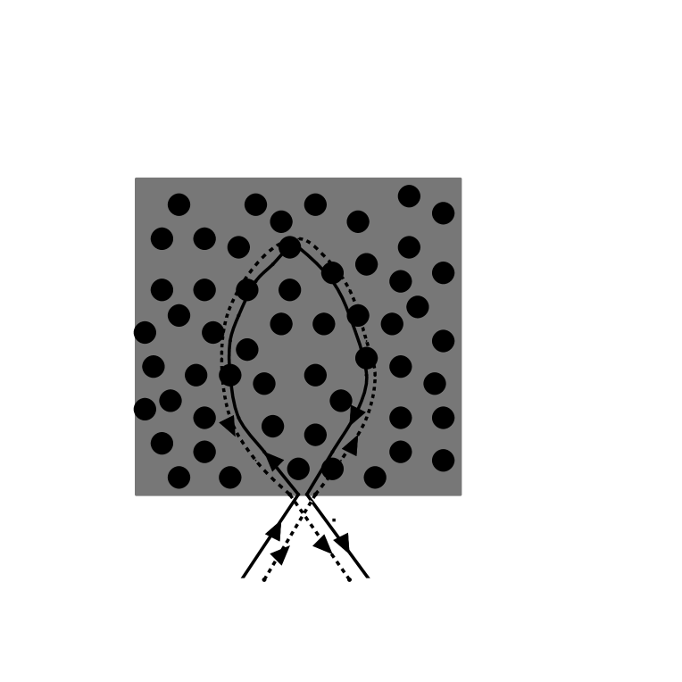
FIG. 1.: Coherently amplifying(marked by shade) medium in presence of disorder. Here we emphasize that the coherent-back-scattering (marked by the loop), hence localization will not be affected due to the presence of coherent amplification. As a result reflected wave will be amplified.

FIG. 2.: A schematic picture of the localization window for a 3D Maxwell wave in $(k,l_{e})$-space, where $k\equiv 2\pi/\lambda$ is the incoming wave vector and $l_{e}$ is the free scattering mean free path . Curve 1 is for weak disorder, never satisfy the Mott-Iofee-Regal (MIR) criterion, i.e $kl_{e}\ll 1$. Curve 2 is for strong disorder case and has a localization window. The two mobility edges are denoted by $a$ and $b$. The point $a$ on the $\lambda$ axis is the correlation length of the disorder. For $\lambda<<a$ (geometric optics limit) the MIR condition for the localization, i.e., $kl_{e}\ll 1$, is not satisfied. For $\lambda>\lambda_{b}$ (the Rayleigh limit) again the MIR criterion is not satisfied due to the weak Rayleigh scattering.

FIG. 3.: Proposal for a lasing scheme using Anderson localization for a non-resonant feedback mechanism: The figure shows a typical 3-level lasing scheme. Proposals for the lasing action are the following: Keep the pumping wave length $\lambda_{p}$, which will excite electrons from the ground state to the excited state, inside the geometrical optic regime. The wave length of the lasing signal $\lambda_{L}$ should lie inside the localization window, as shown in Fig.2

FIG. 4.: Schematic picture of a Fabry-Perot etalon, a resonant cavity for the usual resonant feedback of lasing media. The amplifying medium is kept between the two parallel mirrors which are used as resonators.

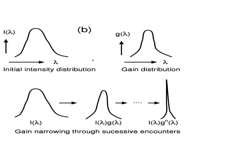
FIG. 5.: (a) A schematic picture in case of non-resonant ”feedback” by feed-forward in a homogeneous amplifying medium. A wave is coherently amplified as it moves forward. The dotted arrows denote the starting wave amplitude and the solid arrows show the coherent addition to the wave amplitude by repeated stimulated emission. (b) A typical gain narrowing process by successive coherent amplifications.

FIG. 6.: Limiting probability distribution $P^{D}_{l\rightarrow\infty}$ of the reflection coefficient $r$, within the random phase approximation, for the cases (a) Coherent absorption ($D=1$), (b) Unitary ($D=0$), and (c) Coherent amplification ($D=-1$).

FIG. 7.: Probability distribution $P(\theta)$ against the active parameter strength $D$ in the weak disorder regime for a fixed disorder parameter strength $2k_{F}\xi=50$ and fixed sample length $l=1$. Plots are for (a) Coherent amplification (D are -ve), and (b) Coherent absorption (D are +ve).

FIG. 8.: Probability distribution $P(r)$ against the sample length $l$, with fixed weak disorder strength $2k_{F}\xi=100$ and fixed weak active parameter $|D|$. Plots are for (a) Coherent amplification (D = -0.5), and (b) Coherent absorption (D = +1).

FIG. 9.: Probability distribution $P(r)$ against the sample length $l$, with fixed weak disorder strength $2k_{F}\xi=100$ and fixed strong active parameter $|D|=10$. Plots are for the cases (a) Coherent amplification (D = -10), and (b) Coherent absorption (D = +10).

FIG. 10.: Probability distribution $P(r)$ and $P(\theta)$ separately against the sample length $l$. Parameters are fixed strong disorder strength $2k_{F}\xi=.001$ and fixed weak active parameter $|D|=0.5$. Plots are for the cases (a) Coherent amplification ($D=-0.5$), and (b) Coherent absorption ($D=+0.5$).

FIG. 11.: Probability distribution $P(r)$ and $P(\theta)$ separately against the sample length $l$. Parameters are fixed strong disorder strength $2k_{F}\xi=.001$ and fixed strong active parameter $|D|=10$. Plots are for the cases (a) Coherent amplification ($D=-10$), and (b) Coherent absorption ($D=+10$)

FIG. 12.: Probability distributions (a) $P(r)$ and (b) $P(\theta)$ against the sample length $l$ with fixed strong disorder strength $2k_{F}\xi=.001$ and fixed weak stochastic absorption parameter $D=0.5$.

FIG. 13.: Probability distributions (a) $P(r)$ and (b) $P(\theta)$ against the sample length $l$ with fixed strong disorder strength $2k_{F}\xi=.001$ and fixed strong stochastic absorption parameter $D=10$.

FIG. 14.: Modeling ”absorption” by fake channels: Channels 1 and 2 are coupled through the current leads to two ”fake” channels 3 and 4 which connect to a thermal reservoir.

REFERENCES

- [1] e-mail pradhan@ee.ucla.edu
- [2] P. W . Anderson, Phys. Rev. 109, 1492 (1958).
- [3] P. A. Lee and T. V. Ramakrishnan Rev. Mod. Phys. 57, 287 (1985).
- [4] For review of localization and multiple scattering see Scattering and localization of classical waves in random media, Ed. Ping Sheng (World Scientific, Singapore, 1990).
- [5] Prabhakar Pradhan, cond-mat/9703255, 1997.
- [6] P. Pradhan and N. Kumar, Phys. Rev. B 50, 5616 (1994).
- [7] M. N. Lawandy, R. M. Balachandran, A. S. L. Gomes and E. Sauvain, Nature, 368, 436 (1994).
- [8] A. Z. Ganack and J. M. Drake, Nature 368, 400 (1994).
- [9] R. M. Balachandran and M. N. Lawandy Opt. Lett. 20, 1271 (1995).
- [10] D. S. Wiersma, M. P. van Albada and A. Lagendijk, Phys. Rev. Lett. 75, 1739 (1995).
- [11] D. S. Wiersma, Ph. D. Thesis, 1995, FOM-Institute for Atomic and Molecular Physics, Amsterdam .
- [12] B. R. Prasad, H. Ramachandran, A. K. Sood, C. K. Subramanian, and N. Kumar, App. Opt. 36, 7718(1997).
- [13] G. Bergmann, Phys. Rep. 107, 1 (1984).
- [14] S. John, Phys. Today 44, 32 (1991); also Physica B 175 , 87 (1991).
- [15] A. F. Ioffe, A. R. Regel, Prog. Semicond. 4, 273 (1960).
- [16] E. Yablonovitch, Phys. Rev. Lett. 58, 2059 (1989).
- [17] S. John, Phys. Rev. Lett. 58, 2486 (1987).
- [18] M. J. Beesley, Laser and their applications (Taylor and Francis Ltd, London, 1976).
- [19] M. Elitzur, Astronomical Masers (Kluwer Academic Publishers, London, 1992).
- [20] J. Summhammer, H. Rauch and M. Zawisky and E. Jericha, Phys. Rev. A 42, 3726 (1990).
- [21] R. L. Weaver, Phys. Rev. B 47, 1077 (1993)
- [22] M. Yosefin, Europhys. Lett. 25, 675 (1994).
- [23] A. M. Jayannavar, Phys. Rev. B 49, 14718 (1994)
- [24] A. Rubio and N. Kumar, Phys. Rev. B 47, 2420 (1993).
- [25] R. Rammal and B. Docout, J. Phys.(Paris),
- [26] Z. Q. Zhang, Phys. Rev. B 52, 7960(1995).
- [27] W. Deng and Z. Q. Zhang, B 55 14230 (1997).
- [28] K. C. Chiu and Z. Q. Zhang, Waves in Random Media 7 635(1997).
- [29] Z. Q. Zhang and K. C. Chiu and D. Zhang, Phys. Rev. B 54, 11891(1996).
- [30] A. K. Gupta and A. M. Jayannavar, Phys. Rev. B 52, 4156(1995).
- [31] S. K. Joshi and A. M. Jayannavar, Phys. Rev. B 56, 12038(1997).
- [32] J. Heinrichs, Phys. Rev. B 56, 8674(1997).
- [33] C. W. J. Beenakker, J. C. J. Paasschens, and P. W. Brouwer, Phys. Rev. Lett. 76, 1368 (1996).
- [34] T. Sh. Misirpaschev, J. C. J. Paasschens and C. W. J. Beenakker, Physica A 236, 189(1997).
- [35] A. A. Burkov and A. Yu. Zyuzin, Phys. Rev. B 55, 5736(1997).
- [36] V. Freilikher, M. Pustilink and I. Yurkevich, cond-mat/9605090 (1996).
- [37] V. Freilikher and M. Pustilink, Phys. Rev. B 55, 653(1997).
- [38] A. K. Sen, Mod. Phys. Lett. B 10, 125(1996).
- [39] K. H. Kim, Preprint.
- [40] M. Buttiker, Phys. Rev. B 33, 3020 (1986).
- [41] R. Hey, K. Maschke and M. Schreiber, Phys. Rev. B 52 8184 (1995).
- [42] O. N. Dorokhov, JETP Lett. 36, 318 (1982); P. A. Mello, P. Pereyra and N. Kumar, Ann. Phys. (N.Y.) 181, 290 (1988).
.