Abstract

In the mean-field approximation, a trapped Bose-Einstein condensate at zero temperature is described by the Gross-Pitaevskii equation for the condensate, or equivalently, by the hydrodynamic equations for the number density and the current density. These equations receive corrections from quantum field fluctuations around the mean field. We calculate the semiclassical corrections to these equations for a general time-independent state of the condensate, extending previous work to include vortex states as well as the ground state. In the Thomas-Fermi limit, the semiclassical corrections can be taken into account by adding a local correction term to the Gross-Pitaevskii equation. At second order in the Thomas-Fermi expansion, the semiclassical corrections can be taken into account by adding local correction terms to the hydrodynamic equations.

1 Introduction

The achievement of Bose-Einstein condensation in trapped atomic vapors [1] has rekindled interest in the theory of nonhomogeneous interacting Bose gases. This problem can be conveniently formulated as a problem in quantum field theory, but the quantum field equations are extremely difficult to solve in general. Fortunately, many of the basic properties of the condensates in existing experiments, such as the density profile of the ground state and the frequencies for small amplitude collective oscillations of the condensate, can be described reasonably well using the mean-field approximation. This approximation reduces the problem to solving the Gross-Pitaevskii equation, a classical equation for the mean field. However, fluctuations of the quantum field around the mean field provide corrections to mean-field predictions that grow as the square root of the number density of the atoms. These corrections will become increasingly important as higher condensate densities are achieved and as the precision of experimental measurements improves. Furthermore, there are some observables, such as the damping rates of collective oscillations, that vanish in the mean-field approximation and are therefore sensitive to the effects of quantum field fluctuations. It is therefore important to understand the effects of quantum field fluctuations, and to be able to calculate them accurately.

The problem of the nonhomogeneous interacting Bose gas at low temperature was studied by Fetter in 1972 [2] using the Bogoliubov approximation. In this approximation, the quantum field equation is linearized around the solution $\phi$ to the Gross-Pitaevskii equation. More elaborate approximations that provide a better extrapolation to higher temperatures, such as the Hartree-Fock-Bogoliubov (HFB) approximation, were developed in the early 1980’s [3, 4]. They require the self-consistent solution of a coupled system of equations consisting of a partial differential equation for $\phi$ and a linear equation for the quantum fluctuation field $\tilde{\psi}$, both of which involve expectation values of operators quadratic in $\tilde{\psi}$. A critical analysis of the HFB approximation and other simpler approximations has recently been given by Griffin [5].

One of the attractive features of the HFB approximation is that it is a conserving approximation that is guaranteed to respect the conservation laws that follow from the symmetries of the field theory. One of the problems with the HFB approximation is that it is not a gapless approximation. In the case of a homogeneous gas, the HFB approximation gives a gap in the spectrum in violation of Goldstone’s theorem. More generally, it fails to respect some of the consequences of the spontaneously broken symmetry of the theory. The classification of approximation methods for a Bose gas according to whether they are conserving or gapless approximations was first made by Hohenberg and Martin [6]. A controlled approximation that corresponds to the truncation of a systematic expansion in a small parameter is guaranteed to be gapless. However such approximations are typically not conserving, because the conservation laws may be satisfied only up to corrections that are higher order in the expansion parameter.

Another problem with the HFB approximation is that solving the HFB equations is a complicated computational problem. It requires solving the partial differential equation for $\phi$, solving the eigenvalue equations for all the normal modes of $\tilde{\psi}$, calculating expectation values of operators quadratic in $\tilde{\psi}$, and iterating this sequence of calculations until they are self-consistent. The resulting solutions for $\phi$ and for the normal modes of $\tilde{\psi}$ contain a great deal of information. Unfortunately, because the HFB approximation is not gapless, some of that information is qualitatively wrong. Furthermore, much of that information is not easily accessible in experiments. For example, the total contribution to the number density from all the normal modes is easier to measure than the contribution from individual normal modes.

It would be worthwhile to develop an improved treatment of the nonhomogeneous interacting Bose gas that avoids the inconsistencies of the HFB approximation and is also computationally simpler. It was shown in Ref. [7] that the effects of quantum field fluctuations on the ground state can be taken into account by adding local correction terms to the partial differential equations of the mean-field approximation. The consistency of the approach was guaranteed by using only controlled approximations. The enormous simplification compared to the HFB approximation comes at the expense of any direct information on the individual normal modes of the quantum fluctuation field. In this paper, we extend the results of Ref. [7] to arbitrary time-independent states of the Bose-Einstein condensate at zero temperature, including vortex states. We also streamline the derivations in Ref. [7] by using dimensional regularization to control infrared and ultraviolet divergences.

The controlled approximations that guarantee the consistency of our approach are based on truncations of systematic expansions in two small quantities. The first of these quantities is $[64\rho({\bf r})a^{3}/\pi]^{1/2}$, where $a$ is the S-wave scattering length and $\rho$ is the number density. This quantity is a local measure of the magnitude of the effects of quantum field fluctuations. We restrict our analysis to the semiclassical approximation, in which the expansion is truncated at first order in $\sqrt{\rho a^{3}}$. The second small quantity is $\xi/R$, where $\xi=[16\pi a\rho({\bf r})]^{-1/2}$ is the local coherence length and $R$ is the length scale for significant variations in $\rho({\bf r})$. The expansion in $\xi/R$ defines the Thomas-Fermi approximation. The effects of quantum field fluctuations are dominated by modes with wavelengths of order $\xi$. The quantity $\xi/R$ is therefore a measure of how local the effects of the quantum field fluctuations are.

In present experiments with Bose-Einstein condensates, the largest values of the semiclassical expansion parameter have been achieved for condensates of Na²³. The scattering length of Na²³ is $a=2.75$ nm. In the experiment of Ref. [8], the peak density that was achieved was approximately $\rho=3\times 10^{15}$ atoms/cm³. The peak value of the semiclassical expansion parameter is therefore $(64\rho a^{3}/\pi)^{1/2}=0.04$. This is small but still large enough that semiclassical corrections should be observable in quantities that can be measured with high precision, such as the collective excitation frequencies of the condensate. The value of the coherence length $\xi$ at the peak density is $[16\pi a\rho({\bf r})]^{-1/2}=5\times 10^{-6}$ cm. The transverse radius $R$ of the elongated condensate was roughly $3\times 10^{-3}$ cm. Thus the Thomas-Fermi expansion parameter $\xi/R$ at the peak density is roughly 0.02. The sizes of the expansion parameters can be controlled by adjusting the shape of the trapping potential and the number of atoms in the trap. The number density that can be achieved is limited however by the loss of atoms from the trap due to 3-body collisions. The size of the expansion parameters can also be controlled by changing the scattering length of the atoms. For example, the use of Feshbach resonances to change the scattering length of Na²³ atoms has already been demonstrated [9].

In the mean-field approximation, the condensate $\phi$ for a time-independent state of a Bose-Einstein condensate in an external potential $V({\bf r})$ satisfies the Gross-Pitaevskii equation:

$$0\;=\;\left({\hbar^{2}\over 2m}\nabla^{2}+\mu-V\right)\phi\;-\;{4\pi\hbar^{2}a\over m}|\phi|^{2}\phi,$$ (1)

where $a$ is the S-wave scattering length and $\mu$ is the chemical potential. This equation can be written equivalently in the hydrodynamic form that consists of a pair of coupled partial differential equations for the number density $\rho=|\phi|^{2}$ and the current density ${\bf j}=-i(\phi^{*}\nabla\phi-\phi\nabla\phi^{*})$:

$$\mu = V\;+\;{4\pi\hbar^{2}a\over m}\rho\;+\;{\hbar^{2}\over 8m\rho^{2}}\left[-2\rho\nabla^{2}\rho+(\nabla\rho)^{2}\right]\;+\;{m\over 2\rho^{2}}{\bf j}^{2},$$ (2)

$$0 = \nabla\cdot{\bf j}.$$ (3)

We calculate the corrections to the mean-field equations from quantum field fluctuations using the semiclassical approximation, which includes all terms through first order in $\sqrt{\rho a^{3}}$. We use the Thomas-Fermi expansion to express the corrections in terms of local quantities. In the Thomas-Fermi limit, we find that the quantum field fluctuations can be taken into account by adding a local correction term to the Gross-Pitaevskii equation (1):

$$0\;=\;\left({\hbar^{2}\over 2m}\nabla^{2}+\mu-V\right)\phi\;-\;{4\pi\hbar^{2}a\over m}|\phi|^{2}\phi\left[1+{5\over 3}\left({64a^{3}\over\pi}\right)^{1/2}|\phi|\right].$$ (4)

At second order in the Thomas-Fermi expansion, the correction term is no longer local when expressed in terms of $\phi$. However there are also nonlocal terms in the relation between $\rho$ and $\phi$. We find that the nonlocal terms cancel to give a local correction term to the hydrodynamic form of the mean-field equations. The current density ${\bf j}$ still satisfies the continuity equation (3), while (2) is replaced by

$$\mu = V\;+\;{4\pi\hbar^{2}a\over m}\rho\;+\;{\hbar^{2}\over 8m\rho^{2}}\left[-2\rho\nabla^{2}\rho+(\nabla\rho)^{2}\right]\;+\;{m\over 2\rho^{2}}{\bf j}^{2}$$ (5)

$$\;+\;\left({64a^{3}\rho\over\pi}\right)^{1/2}\left({16\pi\hbar^{2}a\over 3m}\rho\;-\;{17\hbar^{2}\over 576m\rho^{2}}\left[-4\rho\nabla^{2}\rho+(\nabla\rho)^{2}\right]\right)\,.$$

This equation was derived previously in Ref. [7] for the special case of the ground state for which ${\bf j}$ vanishes. In this paper, we extend that derivation to a general time-independent state with a nonvanishing current. We find a remarkable cancellation of the $\bf j$-dependent terms in the semiclassical correction, so that the dependence on the current $\bf j$ enters only through the classical terms.

We begin in Section 2 by writing down the general equations that determine the condensate, the number density, and the current density for a time-independent state of a Bose-Einstein condensate in an external potential. In Section 3, we set up a perturbative framework for calculating the local effects of quantum field fluctuations when they are dominated by wavelengths comparable to the coherence length. The semiclassical approximation is introduced in Section 4. The equation for the condensate in this approximation is expressed in terms of $\rho$, ${\bf j}$, and expectation values involving the quantum fluctuation field. The Thomas-Fermi expansion is used in Section 5 to calculate the expectation values to second order in the gradient expansion. Inserting these expectation values into the semiclassical equation, we obtain our final result (5). In Section 6, we deduce the corresponding equation for the condensate $\phi$ and show that it is logarithmicly sensitive to wavelengths much larger than the coherence length. Finally, in Section 7, we summarize our results and discuss some possible generalizations. Calculational details related to the evaluation of Feynman diagrams are collected in two appendices. In Appendix A, we give expressions for momentum integrals with dimensional regularization used for both an infrared and an ultraviolet cutoff. In Appendix B, we illustrate the use of Feynman diagrams to calculate the coefficients in the Thomas-Fermi expansions of the expectation values of local quantum field operators. The coefficients that appear in the equations for the mean field and for the hydrodynamic variables are given in terms of dimensionally regularized integrals in Appendix C.

2 Static Bose-Einstein condensate

The problem of the Bose-Einstein condensation of a large number $N$ of identical atoms in a trapping potential $V({\bf r})$ can be formulated in terms of a quantum field theory with a single complex field $\psi({\bf r},t)$. The quantum field satisfies

$$i\dot{\psi}\;+\;\left[\nabla^{2}+\mu-V({\bf r})\right]\psi\;-\;{g\over 2}(\psi^{\dagger}\psi)\psi\;=\;0.$$ (6)

For simplicity of notation, we have set $\hbar=2m=1$ in (6). Dimensional analysis can be used to reinsert the appropriate factors of $\hbar$ and $2m$ at the end of the calculation. The parameter $g$ in (6) is proportional to the S-wave scattering length $a$ of the atom:

$$g\;=\;{8\pi\hbar^{2}a\over m}\;=\;16\pi a.$$ (7)

The chemical potential $\mu$ in (6) is to be adjusted so that the average number of atoms in the ground state $|0\rangle$ is a specified number $N$:

$$\int d^{3}r\;\langle 0|\psi^{\dagger}\psi|0\rangle\;=\;N.$$ (8)

We now consider an arbitrary time-independent state $|n\rangle$ of the Bose-Einstein condensate at zero temperature. If the potential traps the atoms in a simply-connected region of space, the time-independent states are the ground state and vortex states. In the ground state, the condensate $\phi({\bf r})$ has a constant phase and the current density ${\bf j}({\bf r})$ vanishes. In a vortex state, ${\bf j}$ is nonzero and the phase of $\phi$ changes by a multiple of $2\pi$ along a curve that circumscribes the core of the vortex. If the atoms are trapped in a region that is not simply-connected, there can be more complicated states $|n\rangle$ with time-independent number density and current. We denote the number density and the current density in the state $|n\rangle$ by $\rho$ and ${\bf j}$, respectively:

$$\rho = \langle n|\psi^{\dagger}\psi|n\rangle,$$ (9)

$${\bf j} = -i\;\langle n|\psi^{\dagger}\nabla\psi-\nabla\psi^{\dagger}\psi|n\rangle.$$ (10)

We also denote the condensate, which is the expectation value of $\psi$ in that state, by $\phi$:

$$\phi\;=\;\langle n|\psi|n\rangle.$$ (11)

The quantum fluctuation field $\tilde{\psi}$, which is defined by

$$\psi({\bf r},t)\;=\;\phi({\bf r})\;+\;\tilde{\psi}({\bf r},t),$$ (12)

has a vanishing expectation value: $\langle n|\tilde{\psi}|n\rangle=0$. The quantum field equation (6) can be expressed as a classical field equation for $\phi$ coupled to a quantum field equation for $\tilde{\psi}$:

$$0 = \left[\nabla^{2}+\mu-V\right]\phi\;-\;{g\over 2}\left[|\phi|^{2}\phi+2\langle\tilde{\psi}^{\dagger}\tilde{\psi}\rangle\phi+\langle\tilde{\psi}\tilde{\psi}\rangle\phi^{*}+\langle\tilde{\psi}^{\dagger}\tilde{\psi}\tilde{\psi}\rangle\right],$$ (13)

$$0 = i\dot{\tilde{\psi}}\;+\;\left[\nabla^{2}+\mu-V\right]\tilde{\psi}\;-\;{g\over 2}\left[2|\phi|^{2}\tilde{\psi}+\phi^{2}\tilde{\psi}^{\dagger}+2\phi\left(\tilde{\psi}^{\dagger}\tilde{\psi}-\langle\tilde{\psi}^{\dagger}\tilde{\psi}\rangle\right)\right.$$ (14)

$$\left.+\phi^{*}\left(\tilde{\psi}\tilde{\psi}-\langle\tilde{\psi}\tilde{\psi}\rangle\right)+\left(\tilde{\psi}^{\dagger}\tilde{\psi}\tilde{\psi}-\langle\tilde{\psi}^{\dagger}\tilde{\psi}\tilde{\psi}\rangle\right)\right].$$

The equation (13) for $\phi$ is just the expectation value of (6). The equation (14) for $\tilde{\psi}$ is obtained by subtracting (13) from (6). We have suppressed the state $|n\rangle$ in the expectation values that appear in (13) and (14). Through the remainder of this paper, it will be understood that all expectation values are for the time-independent state $|n\rangle$.

The system of equations consisting of (13) and (14) involves coupled nonlinear equations for $\phi$ and $\tilde{\psi}$ and is extremely difficult to solve in general. We must resort to some approximations to make this system of equations more tractable. The consistency of an approximation will be guaranteed if it is controlled by a small expansion parameter. From the example of the homogeneous Bose gas, it is clear that the fractional size of the effects of quantum field fluctuations is measured locally by the dimensionless quantity $[64{\rho({\bf r})a^{3}}/\pi]^{1/2}$. If the peak value of this quantity is less than one, one can use $\sqrt{\rho a^{3}}$ as an expansion parameter. If we wish to describe the interactions of the atoms in terms of the S-wave scattering length $a$ only, then we are limited to first order in $\sqrt{\rho a^{3}}$. At second order in $\sqrt{\rho a^{3}}$, there are ultraviolet divergences whose renormalization requires additional input parameters, including a pointlike contribution to the $3\to 3$ scattering amplitude [11, 12]. We will refer to the approximation in which we truncate at first order in $\sqrt{\rho a^{3}}$ as the semiclassical approximation.

The semiclassical approximation is defined not by neglecting any particular terms in the equations (13) and (14), but rather by the truncation of the expansion in $\sqrt{\rho a^{3}}$ at first order. This approximation does allow those equations to be simplified, because not all the terms are necessary to achieve first order accuracy, but the simplifications depend on the quantity being calculated. Our goal will be to achieve first order accuracy in quantities like $\phi$, $\rho$, and ${\bf j}$ that can be defined as expectation values of local operators. In terms of Feynman diagrams, first order accuracy requires keeping all contributions from one-loop diagrams, while diagrams with 2 or more loops can be neglected. The expectation value $\langle\tilde{\psi}^{\dagger}\tilde{\psi}\tilde{\psi}\rangle$ receives contributions only from diagrams with 2 or more loops, and it therefore can be omitted in (13). We need to solve the quantum field equation (14) only with enough accuracy to guarantee first order accuracy for the remaining expectation values $\langle\tilde{\psi}^{\dagger}\tilde{\psi}\rangle$ and $\langle\tilde{\psi}\tilde{\psi}\rangle$ in (13). The terms in (14) that are quadratic or cubic in $\tilde{\psi}$ contribute to $\langle\tilde{\psi}^{\dagger}\tilde{\psi}\rangle$ and $\langle\tilde{\psi}\tilde{\psi}\rangle$ only through diagrams with 2 or more loops. We therefore need keep only those terms in (14) that are linear in $\tilde{\psi}$. Thus to the accuracy required, (13) and (14) reduce to

$$0 = \left[\nabla^{2}+\mu-V\right]\phi\;-\;{g\over 2}|\phi|^{2}\phi\;-\;g\langle\tilde{\psi}^{\dagger}\tilde{\psi}\rangle\phi\;-\;{g\over 2}\langle\tilde{\psi}\tilde{\psi}\rangle\phi^{*},$$ (15)

$$0 = i\dot{\tilde{\psi}}\;+\;\left[\nabla^{2}+\mu-V\right]\tilde{\psi}\;-\;g|\phi|^{2}\tilde{\psi}\;-\;{g\over 2}\phi^{2}\tilde{\psi}^{\dagger}.$$ (16)

The expectation value $\langle\tilde{\psi}^{\dagger}\tilde{\psi}\rangle$ in (15) is the noncondensate density, which is the correction to the number density from quantum field fluctuations. The expectation value $\langle\tilde{\psi}\tilde{\psi}\rangle$ is called the anomalous density. It should be emphasized that the equation (16) is not designed to give the normal modes of $\tilde{\psi}$ to any specific accuracy. We need only solve the equation for $\tilde{\psi}$ with sufficient accuracy so that the expectation values in (15) can be calculated with an error that is second order in $\sqrt{\rho a^{3}}$ relative to $|\phi|^{2}$. Since these expectation values are dominated by modes with wavelengths comparable to the coherence length $\xi$, the equation for $\tilde{\psi}$ need only be accurate for wavelengths of order $\xi$.

We now compare the accuracy of the semiclassical equations (15) and (16) to the traditional approximations to the full equations (13) and (14). While the main purpose of the traditional approximations was to take into account the effects of nonzero temperature, it is instructive to determine their accuracy at zero temperature. The Bogoliubov approximation is defined by the equations (15) and (16), with the expectation values set to zero in (15). Thus $\phi$ satisfies the Gross-Pitaevskii equation. The solution to this equation gives $\phi({\bf r})$ with a fractional error that is first order in $\sqrt{\rho a^{3}}$. In contrast, the solution to the semiclassical equations (15) and (16) gives $\phi$ with a fractional error that is second order in $\sqrt{\rho a^{3}}$.

In the Hartree-Fock-Bogoliubov (HFB) approximation, the $\langle\tilde{\psi}^{\dagger}\tilde{\psi}\tilde{\psi}\rangle$ term in (13) is neglected so that it reduces to (15) and the products of field operators in (14) are replaced by terms in which pairs of operators have been contracted into expectation values:

$$0\;=\;i\dot{\tilde{\psi}}\;+\;\left[\nabla^{2}+\mu-V\right]\tilde{\psi}\;-\;g\left[|\phi|^{2}+\langle\tilde{\psi}^{\dagger}\tilde{\psi}\rangle\right]\tilde{\psi}\;-\;{g\over 2}\left[\phi^{2}+\langle\tilde{\psi}\tilde{\psi}\rangle\right]\tilde{\psi}^{\dagger}.$$ (17)

Solving the system of equations (15) and (17) is a complicated numerical problem. It requires making an initial guess for $\phi$ and for the infinitely many normal modes of $\tilde{\psi}$, calculating the expectation values $\langle\tilde{\psi}^{\dagger}\tilde{\psi}\rangle$ and $\langle\tilde{\psi}\tilde{\psi}\rangle$, solving (15) for $\phi$, solving (17) for the normal modes of $\tilde{\psi}$, and iterating this sequence of calculations until they are self-consistent. The net effect of the additional terms in (17) that do not appear in (16) is to include a subset of corrections that are second order or higher in $\sqrt{\rho a^{3}}$. Since there are other corrections that are second order in $\sqrt{\rho a^{3}}$ that have not been included, the use of (17) in conjunction with (15) does not improve the accuracy in the determination of $\phi$. If all the second order corrections were uniformly small in $\sqrt{\rho a^{3}}$, it would do no harm to include only some of them. Unfortunately, there are individual correction terms that diverge in the limit $\xi/R\to 0$, but which cancel when all terms of a given order in $\sqrt{\rho a^{3}}$ are added together. Including some but not all of the second order terms is dangerous, because one may omit some of the terms that are necessary for the cancellations. Thus, by including a subset of the higher order corrections, the HFB approximation may actually decrease the accuracy. This problem can be avoided by using a controlled approximation, because any such cancellations will occur order by order in the expansion parameter.

The fact that the HFB approximation is not a controlled approximation is reflected at nonzero temperature in the existence of an energy gap in the spectrum of the hamiltonian for $\tilde{\psi}$, which contradicts Goldstone’s theorem. In the Popov approximation, the energy gap is eliminated by setting the anomalous density $\langle\tilde{\psi}\tilde{\psi}\rangle$ to zero in (15) and (17). The resulting error in $\phi$ is first order in $\sqrt{\rho a^{3}}$. Thus at zero temperature, the Popov approximation is no more accurate than the Bogoliubov approximation, despite the fact that it requires much more complicated calculations. In the approximation used by Goldman et al. in Ref. [3], the $\langle\tilde{\psi}\tilde{\psi}\rangle$ term in (15) was set to zero. Thus it also gives an error in $\phi$ that is first order in $\sqrt{\rho a^{3}}$.

The semiclassical equations (15) and (16) can be greatly simplified by using a further approximation that is also controlled by a small expansion parameter. The effects of quantum field fluctuations are dominated by wavelengths comparable to the local coherence length $\xi=[16\pi\rho({\bf r})a]^{-1/2}$. For the ground state of a Bose-Einstein condensate containing $N$ atoms, $\xi$ scales like $N^{-1/5}$, where $N$ is the number of atoms in the trap [10]. In contrast, the length scale $R$ for significant variations in $\rho({\bf r})$ grows like $N^{1/5}$. If $N$ is sufficiently large, $\xi$ is much shorter than $R$. This justifies an expansion in powers of $\xi/R$ or, equivalently, in powers of gradients of $\phi$. This expansion defines the Thomas-Fermi approximation. We will calculate the semiclassical corrections through second order in the Thomas-Fermi expansion.

In the Thomas-Fermi limit, the semiclassical equation (15) for the condensate becomes particularly simple. As we shall see, the expectation values at leading order in $\xi/R$ are simply functions of $\phi$:

$$\langle\tilde{\psi}^{\dagger}\tilde{\psi}\rangle \approx {1\over 24\pi^{2}}g^{3/2}|\phi|^{3},$$ (18)

$$\langle\tilde{\psi}\tilde{\psi}\rangle \approx {1\over 8\pi^{2}}g^{3/2}|\phi|\phi^{2}.$$ (19)

Inserting the expectation values (18) and (19) into (15), it reduces to a partial differential equation for $\phi$. Using dimensional analysis to reinsert the appropriate factors of $2m$ and $\hbar$, we obtain the equation (4), which is simply the Gross-Pitaevskii equation with a correction term that corresponds to the local density approximation.

To go to second order in the Thomas-Fermi expansion, we need to include terms in the expectation values (18) and (19) that are second order in gradients of $\phi$. As we shall see, the coefficients of these terms are logarithmicly infrared divergent, indicating a sensitivity to length scales much greater than $\xi$. This sensitivity can be reduced by expressing the equation (15) in terms of the hydrodynamic variables $\rho$ and ${\bf j}$ defined by (9) and (10):

$$\rho = |\phi|^{2}\;+\;\langle\tilde{\psi}^{\dagger}\tilde{\psi}\rangle,$$ (20)

$${\bf j} = -i\left(\phi^{*}\nabla\phi-\phi\nabla\phi^{*}\right)\;-\;i\langle\tilde{\psi}^{\dagger}\nabla\tilde{\psi}-\nabla\tilde{\psi}^{\dagger}\tilde{\psi}\rangle.$$ (21)

We will find that if the condensate $\phi$ in (15) is eliminated in favor of $\rho$ and ${\bf j}$, the infrared divergences cancel and the equation reduces to (5). We will obtain this result in two different ways. In Sections 4 and 5, we organize the calculation so that (15) gives directly our final equation (5) for $\rho$ and ${\bf j}$. In Section 6, we calculate the expectation values (18) and (19) to second order in the Thomas-Fermi expansion using an infrared cutoff. We then use the condensate equation (15) to deduce our final equation (5) for $\rho$ and ${\bf j}$.

3 Perturbative framework

In this section, we set up a perturbative framework that can be used to calculate the leading effects of quantum field fluctuations. This framework involves introducing an arbitrary momentum scale $\Lambda$ that will later be chosen to be the inverse of the local coherence length $\xi$. The perturbation series is an expansion in powers of $g\Lambda$, and the semiclassical approximation introduced in Section 4 is the truncation of that expansion at first order in $g\Lambda$.

The quantum field theory associated with the equation (6) is summarized by the action

$$S[\psi]\;=\;\int dt\int d^{3}x\left\{{i\over 2}\left(\psi^{\dagger}\dot{\psi}-\dot{\psi}^{\dagger}\psi\right)-\nabla\psi^{\dagger}\cdot\nabla\psi\;+\;\left[\mu-V({\bf r})\right]\psi^{\dagger}\psi\;-\;{g\over 4}(\psi^{\dagger}\psi)^{2}\right\}.$$ (22)

This action is invariant under the $U(1)$ symmetry in which the field is multiplied by a phase:

$$\psi({\bf r},t)\;\longrightarrow\;e^{i\alpha}\psi({\bf r},t).$$ (23)

The action is also invariant under time-reversal symmetry:

$$\psi({\bf r},t)\;\longrightarrow\;\psi^{\dagger}({\bf r},-t).$$ (24)

The $U(1)$ symmetry (23) guarantees that the number density and the current density satisfy the continuity equation:

$$\dot{\rho}\;+\;\nabla\cdot{\bf j}\;=\;0.$$ (25)

A $U(1)$ symmetry transformation can also be used to make the condensate $\phi({\bf r})=\langle\psi({\bf r})\rangle$ real-valued at any specific point ${\bf r}_{0}$.

The quantum field theory defined by (22) has ultraviolet divergences that must be removed by renormalizations of the parameters $\mu$ and $g$. There is also an ultraviolet divergence in the number density that can be removed either by renormalization or by an operator-ordering prescription. In Ref. [7], the effects of quantum field fluctuations on the ground state were calculated using a momentum cutoff to regularize the ultraviolet divergences. The divergences were cancelled explicitly by counterterms for $\mu$, $g$, and $\rho$. In this paper, we choose to regularize the ultraviolet divergences using dimensional regularization, which involves calculating integrals as analytic functions of the number of dimensions $D$ and then analytically continuing them to $D=3$. This method has been used to calculate the properties of a homogeneous Bose gas [13, 12] and it greatly streamlines the calculations. One advantage of dimensional regularization is that it sets integrals that diverge like a power of the ultraviolet cutoff, and involve no other momentum scales, equal to zero. Since the counterterms for $\mu$, $g$, and $\rho$ are pure power ultraviolet divergences, they are identically zero in dimensional regularization. We have therefore omitted counterterms for the parameters $g$ and $\mu$ in (22).

It is convenient to decompose both the condensate (11) and the quantum fluctuation field $\tilde{\psi}$ defined by (12) into real and imaginary parts:

$$\phi({\bf r}) = v({\bf r})+iw({\bf r}),$$ (26)

$$\tilde{\psi}({\bf r},t) = {\xi({\bf r},t)+i\eta({\bf r},t)\over\sqrt{2}}.$$ (27)

In the neighborhood of a point ${\bf r}_{0}$ where $w$ vanishes, we can identify $\xi$ and $\eta$ as the quantum fluctuation fields associated with the number density and with the phase of the condensate, respectively. Inserting these expressions into the action (22) and expanding in powers of $\xi$ and $\eta$, we obtain a condensate term $S[v+iw]$ and terms up to fourth order in $\xi$ and $\eta$. The equations (12) and (27) define the Cartesian parameterization of the quantum field $\psi$ in terms of real quantum fields. One could equally well use an alternative parameterization, such as the polar parameterization:

$$\psi({\bf r},t)\;=\;\left[v^{2}({\bf r})+\sigma({\bf r},t)\right]^{1/2}e^{i\theta({\bf r})}e^{i\alpha({\bf r,t})},$$ (28)

where $v$ and $\theta$ are real classical fields, while $\sigma$ and $\alpha$ are real quantum fields. The polar parameterization has the advantage in perturbative calculations that it eliminates infrared divergences that with other parameterizations cancel only after adding Feynman diagrams [14]. If we use controlled approximations based on systematic expansions in small quantities, any parameterization should lead to the same results for physical quantities. In Ref. [7], it was verified explicitly that the Cartesian and polar parameterizations give the same final equation for the number density in the ground state. Since the calculations were simpler using the Cartesian parameterization, we use only that parameterization in this paper.

If the system is near the Thomas-Fermi limit, the length scale for significant changes in the condensate is large compared to the local coherence length $(g\rho)^{-1/2}$. At any specific point ${\bf r}_{0}$ inside the condensate, the short-wavelength modes of the quantum fields $\xi$ and $\eta$ behave locally like those of a homogeneous Bose gas with coherence length $[g\rho({\bf r}_{0})]^{-1/2}$. Their dispersion relation can be approximated by the Bogoliubov dispersion relation

$$\epsilon(k)\;=\;k\sqrt{k^{2}+\Lambda^{2}},$$ (29)

with $\Lambda^{2}\approx g\rho({\bf r}_{0})$. A particle with the dispersion relation (29) is described by a free field theory with the action

$$S_{\mbox{\footnotesize free}}[\xi,\eta]\;=\;\int dt\int d^{3}x\left\{{1\over 2}\left(\eta\dot{\xi}-\xi\dot{\eta}\right)\;-\;{1\over 2}\left[(\nabla\xi)^{2}+\Lambda^{2}\xi^{2}+(\nabla\eta)^{2}\right]\right\}.$$ (30)

We can express the complete action (22) as the sum of the background term $S[v+iw]$, the free action (30) for the quantum fields, and an interaction term:

$$S[\psi]\;=\;S[v+iw]\;+\;S_{\mbox{\footnotesize free}}[\xi,\eta]\;+\;S_{\mbox{\footnotesize int}}[v,w,\xi,\eta].$$ (31)

The last term describes the interaction of the Bogoliubov modes with each other and with sources that depend on $v$ and $w$:

$$S_{\mbox{\footnotesize int}}[v,w,\xi,\eta]\;=\;\int dt\int d^{3}x\left\{\sqrt{2}(T\xi+S\eta)\;+\;{1\over 2}(X\xi^{2}+Y\eta^{2}+2R\xi\eta)\right.$$

$$\left.\;+\;{1\over\sqrt{2}}(Z\xi+Q\eta)(\xi^{2}+\eta^{2})\;-\;{g\over 16}(\xi^{2}+\eta^{2})^{2}\right\}.$$ (32)

The sources are

$$T = \left[\mu-V({\bf r})-{g\over 2}(v^{2}+w^{2})\right]v+\nabla^{2}v,$$ (33)

$$S = \left[\mu-V({\bf r})-{g\over 2}(v^{2}+w^{2})\right]w+\nabla^{2}w,$$ (34)

$$X = \Lambda^{2}+\mu-V({\bf r})-{g\over 2}(3v^{2}+w^{2}),$$ (35)

$$Y = \mu-V({\bf r})-{g\over 2}(v^{2}+3w^{2}),$$ (36)

$$Z = -{g\over 2}v,$$ (37)

$$Q = -{g\over 2}w,$$ (38)

$$R = -gvw.$$ (39)

The sources $T$ and $S$ are simply the real and imaginary parts of the Gross-Pitaevskii equation for the condensate $v+iw$. Note that the dependence of the source $X$ on $\Lambda^{2}$ precisely cancels the $\Lambda$–dependence of the free action (30). Thus $\Lambda$ is a completely arbitrary parameter. That arbitrariness will be exploited below to ensure that the terms in (32) can be treated as perturbations.

The quantum field equations for $\xi$ and $\eta$ are obtained by varying the action (31). Taking the expectation value of those quantum field equations and using the fact that $\xi$ and $\eta$ have vanishing expectation values, we obtain a pair of equations equivalent to (13):

$$0 = T\;+\;{1\over 2}Z\langle 3\xi^{2}+\eta^{2}\rangle\;+\;Q\langle\xi\eta\rangle\;-\;{g\over 4\sqrt{2}}\langle\xi(\xi^{2}+\eta^{2})\rangle,$$ (40)

$$0 = S\;+\;{1\over 2}Q\langle\xi^{2}+3\eta^{2}\rangle\;+\;Z\langle\xi\eta\rangle\;-\;{g\over 4\sqrt{2}}\langle\eta(\xi^{2}+\eta^{2})\rangle.$$ (41)

We will refer to these as the tadpole equations for $\xi$ and for $\eta$, respectively. The quantum field equations for $\xi$ and $\eta$ that correspond to (14) are

$$0 = \dot{\xi}\;+\;(\nabla^{2}+Y)\eta\;+\;R\xi\;+\;{1\over\sqrt{2}}Q\left(\xi^{2}+3\eta^{2}-\langle\xi^{2}+3\eta^{2}\rangle\right)$$ (42)

$$\;+\;\sqrt{2}Z\left(\xi\eta-\langle\xi\eta\rangle\right)\;-\;{g\over 4}\left(\eta(\xi^{2}+\eta^{2})-\langle\eta(\xi^{2}+\eta^{2})\rangle\right),$$

$$0 = -\dot{\eta}\;+\;(\nabla^{2}-\Lambda^{2}+X)\xi\;+\;R\eta\;+\;{1\over\sqrt{2}}Z\left(3\xi^{2}+\eta^{2}-\langle 3\xi^{2}+\eta^{2}\rangle\right)$$ (43)

$$\;+\;\sqrt{2}Q\left(\xi\eta-\langle\xi\eta\rangle\right)\;-\;{g\over 4}\left(\xi(\xi^{2}+\eta^{2})-\langle\xi(\xi^{2}+\eta^{2})\rangle\right).$$

The expressions (20) and (21) for the number density and the current density can be written as

$$\rho = v^{2}+w^{2}+{1\over 2}\langle\xi^{2}+\eta^{2}\rangle,$$ (44)

$${\bf j} = 2\left(v\nabla w-w\nabla v\right)\;+\;\langle\xi\nabla\eta-\eta\nabla\xi\rangle.$$ (45)

Our strategy will be to solve the quantum field equations (42) and (43), treating the terms in (32) as perturbations, and then to calculate the expectation values in (40), (41), (44), and (45) to first order in $g\Lambda$.

4 Semiclassical approximation

For the perturbation theory defined by the decomposition of the action (31) into free and interaction parts, the appropriate dimensionless expansion parameter is the product of the coupling constant $g$ and the coherence scale $\Lambda$. The semiclassical approximation is defined by truncating the expansion in powers of $g\Lambda$ at first order. If the dimensionless ratio $\Lambda/\sqrt{g\rho}$ is held fixed, this is equivalent to truncating at first order in $\sqrt{\rho a^{3}}$. In terms of Feynman diagrams, accuracy to first order in $g\Lambda$ corresponds to keeping only the contributions from one-loop diagrams. The expectation values in (40) and (41) that are cubic in $\xi$ and $\eta$ receive contributions only from diagrams with 2 or more loops and therefore can be omitted. Thus the tadpole equations reduce to

$$0 = T\;+\;{1\over 2}Z\langle 3\xi^{2}+\eta^{2}\rangle\;+\;Q\langle\xi\eta\rangle,$$ (46)

$$0 = S\;+\;{1\over 2}Q\langle\xi^{2}+3\eta^{2}\rangle\;+\;Z\langle\xi\eta\rangle.$$ (47)

We will refer to these equations as the semiclassical tadpole equations for $\xi$ and $\eta$, respectively. In the quantum field equations (42) and (43), the terms that are quadratic or cubic in $\xi$ and $\eta$ contribute to the expectation values in (46) and (47) only through diagrams with 2 or more loops. We therefore need to keep only the linear terms in the quantum field equations:

$$0 = \dot{\xi}\;+\;(\nabla^{2}+Y)\eta\;+\;R\xi,$$ (48)

$$0 = -\dot{\eta}\;+\;(\nabla^{2}-\Lambda^{2}+X)\xi\;+\;R\eta.$$ (49)

These equations describe the propagation of the fields $\xi$ and $\eta$ in the presence of the sources $X$, $Y$, and $R$, but with no other interactions. Note that the explicit dependence of (49) on $\Lambda$ is cancelled by the $\Lambda$–dependence of the source $X$. We will find that a judicious choice of $\Lambda$ will allow the source $X$ to be treated as a perturbation, along with $Y$ and $R$. The expectation values that appear in the semiclassical tadpole equations (46) and (47) and in the expressions for $\rho$ and ${\bf j}$ in (44) and (45) are functionals of the sources $X$, $Y$, and $R$. Under the time-reversal symmetry (24), $\xi$, $X$, and $Y$ are even, while $\eta$ and $R$ are odd. The expectation values $\langle\xi^{2}\rangle$ and $\langle\eta^{2}\rangle$ are therefore even functionals of $R$, while $\langle\xi\eta\rangle$ and $\langle\xi\nabla\eta-\eta\nabla\xi\rangle$ are odd functionals of $R$.

Since the sources $X$, $Y$, and $R$ depend on $v$ and $w$, the expectation values in (44)–(47) are functionals of $v$ and $w$. In order to obtain an equation for $\rho$ and ${\bf j}$, we will use (44) and (45) to eliminate $v$ and $w$ from (46) and (47) in favor of $\rho$ and ${\bf j}$. The expectation values that appear in these equations are the corrections to the classical equations from quantum field fluctuations. They are smaller than individual terms in the classical equations by a factor of $\sqrt{\rho a^{3}}$. The semiclassical approximation includes all terms through first order in $\sqrt{\rho a^{3}}$. In the course of manipulating the equations (44)–(47) to eliminate $v$ and $w$, there is no loss of accuracy if we expand the resulting expressions to first order in the expectation values, dropping higher order terms. The resulting equations still includes all effects of quantum field fluctuations through first order in $\sqrt{\rho a^{3}}$. Solving (44) and (45) for $v$ and $\nabla w$ and expanding to first order in the expectation values, we obtain

$$v = (\rho-w^{2})^{1/2}\;-\;{1\over 4(\rho-w^{2})^{1/2}}\langle\xi^{2}+\eta^{2}\rangle,$$ (50)

$$\nabla w = {1\over 2v}({\bf j}+2w\nabla v)\;-\;{1\over 2v}\langle\xi\nabla\eta-\eta\nabla\xi\rangle.$$ (51)

We can derive analogous expressions for $\nabla v$, $\nabla^{2}v$, and $\nabla^{2}w$ by differentiating (50) and (51). By substituting iteratively and expanding to first order in the expectation values, we can eliminate $v$, $\nabla v$, $\nabla^{2}v$, $\nabla w$, and $\nabla^{2}w$ from the right side of the equation in favor of $\rho$, ${\bf j}$, their derivatives, and also $w$. The resulting expressions at a specific point ${\bf r}_{0}$ become particularly simple if we use a global phase transformation to set $w({\bf r}_{0})=0$:

$$v({\bf r}_{0}) = {1\over 4\rho^{1/2}}\left[4\rho\;-\;\langle\xi^{2}+\eta^{2}\rangle\right],$$ (52)

$$\nabla v({\bf r}_{0}) = {1\over 8\rho^{3/2}}\left[4\rho\nabla\rho\;+\;\nabla\rho\langle\xi^{2}+\eta^{2}\rangle\;-\;2\rho\nabla\langle\xi^{2}+\eta^{2}\rangle\right],$$ (53)

$$\nabla^{2}v({\bf r}_{0}) = {1\over 16\rho^{5/2}}\left[-4\rho[-2\rho\nabla^{2}\rho+(\nabla\rho)^{2}+{\bf j}^{2}]\;-\;[-2\rho\nabla^{2}\rho+3(\nabla\rho)^{2}+3{\bf j}^{2}]\langle\xi^{2}+\eta^{2}\rangle\right.$$ (54)

$$\left.\;+\;4\rho\nabla\rho\cdot\nabla\langle\xi^{2}+\eta^{2}\rangle\;-\;4\rho^{2}\nabla^{2}\langle\xi^{2}+\eta^{2}\rangle\;+\;8\rho{\bf j}\cdot\langle\xi\nabla\eta-\eta\nabla\xi\rangle\right],$$

$$w({\bf r}_{0}) = 0,$$ (55)

$$\nabla w({\bf r}_{0}) = {1\over 8\rho^{3/2}}\left[4\rho{\bf j}\;+\;{\bf j}\langle\xi^{2}+\eta^{2}\rangle\;-\;4\rho\langle\xi\nabla\eta-\eta\nabla\xi\rangle\right],$$ (56)

$$\nabla^{2}w({\bf r}_{0}) = {1\over 8\rho^{3/2}}\left[4\rho\nabla\cdot{\bf j}\;+\;\nabla\cdot{\bf j}\langle\xi^{2}+\eta^{2}\rangle\;-\;4\rho\nabla\cdot\langle\xi\nabla\eta-\eta\nabla\xi\rangle\right].$$ (57)

Inserting the expressions (52)–(57) into (46) and (47) and expanding to first order in the expectation values, we obtain expressions for the tadpole equations at the point ${\bf r}_{0}$ with $v$ and $w$ eliminated in favor of $\rho$ and ${\bf j}$. The semiclassical tadpole equation (47) for $\eta$ reads

$$0\;=\;{1\over 8\rho^{3/2}}\left[4\rho\nabla\cdot{\bf j}\;+\;\nabla\cdot{\bf j}\,\langle\xi^{2}+\eta^{2}\rangle\;-\;4g\rho^{2}\,\langle\xi\eta\rangle\;-\;4\rho\nabla\cdot\langle\xi\nabla\eta-\eta\nabla\xi\rangle\right].$$ (58)

The last term in (58) can be simplified by using the quantum field equations (48) and (49) for $\xi$ and $\eta$:

$$\nabla\cdot\langle\xi\nabla\eta-\eta\nabla\xi\rangle = \langle\xi\nabla^{2}\eta-\eta\nabla^{2}\xi\rangle$$ (59)

$$= -{1\over 2}{d\ \over dt}\langle\xi^{2}+\eta^{2}\rangle\;+\;(X-Y-\Lambda^{2})\langle\xi\eta\rangle\;-\;R\langle\xi^{2}-\eta^{2}\rangle$$

$$= -g(v^{2}-w^{2})\langle\xi\eta\rangle\;-\;gvw\langle\xi^{2}-\eta^{2}\rangle.$$

In the last step, we have used the expressions (35), (36), and (39) for the sources and the fact that $\langle\xi^{2}+\eta^{2}\rangle$ is time-independent. Since $w$ vanishes at the point ${\bf r}_{0}$ and $\rho-v^{2}$ is of order $\sqrt{\rho a^{3}}$ at that point, (59) reduces to $-g\rho\langle\xi\eta\rangle$, up to terms that are second order in $\sqrt{\rho a^{3}}$. Thus the last two terms in (58) cancel. Up to an overall multiplicative factor, the first two terms in (58) reduce to the time-independent continuity equation $\nabla\cdot{\bf j}=0$.

The semiclassical tadpole equation (46) for $\xi$ at the point ${\bf r}_{0}$ reduces to

$$0 = \left(\mu-V-{g\over 2}\rho-{1\over 4\rho^{2}}\left[-2\rho\nabla^{2}\rho+(\nabla\rho)^{2}+{\bf j}^{2}\right]\right)\rho^{1/2}$$ (60)

$$\;-\;{g\over 2}\rho^{1/2}\,\langle\xi^{2}\rangle\;-\;{1\over 4\rho^{5/2}}\left[-\rho\nabla^{2}\rho+(\nabla\rho)^{2}+{\bf j}^{2}\right]\langle\xi^{2}+\eta^{2}\rangle$$

$$\;+\;{1\over 4\rho^{3/2}}\nabla\rho\cdot\nabla\langle\xi^{2}+\eta^{2}\rangle\;-\;{1\over 4\rho^{1/2}}\nabla^{2}\langle\xi^{2}+\eta^{2}\rangle\;+\;{1\over 2\rho^{3/2}}{\bf j}\cdot\langle\xi\nabla\eta-\eta\nabla\xi\rangle$$

$$\;-\;{1\over 4\rho^{1/2}}\left(\mu-V-{g\over 2}\rho-{1\over 4\rho^{2}}\left[-2\rho\nabla^{2}\rho+(\nabla\rho)^{2}+{\bf j}^{2}\right]\right)\langle\xi^{2}+\eta^{2}\rangle.$$

The last line in (60) is proportional to the classical tadpole equation, which is just the first line of (60). The classical equation differs from zero by terms of order $\sqrt{\rho a^{3}}$. Since the expectation value in the last line of (60) is also of order $\sqrt{\rho a^{3}}$, the last line is second order in $\sqrt{\rho a^{3}}$ and can be omitted. Alternatively, it can be cancelled by multiplying (60) by $1+\langle\xi^{2}+\eta^{2}\rangle/(4\rho)$ and keeping only those terms that are first order in the expectation values. To complete the derivation of our equations for $\rho$ and ${\bf j}$, we must calculate the expectation values that appear in the remaining terms of (60) and express them in terms of $\rho$ and ${\bf j}$.

5 Thomas-Fermi expansion

In the previous section, the semiclassical tadpole equation for $\xi$ was evaluated at a point ${\bf r}_{0}$ where $w$ vanishes and expressed in terms of $\rho$, ${\bf j}$, and expectation values of operators. In the resulting equation (60), the operators constructed out of quantum fields $\xi$ and $\eta$ that satisfy (48) and (49). In this section, we use the Thomas-Fermi expansion to evaluate the expectation values and reduce (60) to a partial differential equation involving $\rho$ and ${\bf j}$ only.

The expectation values in (60) are functionals of the sources $X$, $Y$, and $R$ given in (35), (36), and (39). We would like to expand the expectation values in powers of the sources and their gradients. The length scale for significant variations in the sources is much greater than the coherence length $(g\rho)^{-1/2}$. The expansion of the expectation values in powers of gradients of the sources is possible if the expectation values receive significant contributions only from modes of the quantum fields $\xi$ and $\eta$ that have wavelengths of order $(g\rho)^{-1/2}$ or less. This can be guaranteed by imposing an infrared cutoff that eliminates the contribution from modes with much longer wavelengths. A dependence on the infrared cutoff indicates a sensitivity to length scales much greater than the coherence length. We will find that the dependence on the infrared cutoff cancels when (60) is expressed in terms of $\rho$ and ${\bf j}$ only.

Our infrared cutoff allows an expectation value at the point ${\bf r}$ to be expanded in powers of gradients of the sources at the point ${\bf r}$, with coefficients that are functions of $X$, $Y$, and $R$ at the point ${\bf r}$. A further expansion in powers of $X$, $Y$, and $R$ is possible if these sources are at least first order in either the gradient expansion or in $\sqrt{\rho a^{3}}$. This is certainly not true in general, but we can make it true at a specific point ${\bf r}_{0}$ by a judicious choice of the arbitrary parameter $\Lambda$. Note that the source $R$ in (39) vanishes at the point ${\bf r}_{0}$ if the $U(1)$ symmetry has been used to set $w({\bf r}_{0})=0$. The sources $X$ and $Y$ in (35) and (36) do not appear to be higher order in the gradient expansion or in $\sqrt{\rho a^{3}}$. However, since the expectation values are already of order $\sqrt{\rho a^{3}}$ and we are keeping only terms to first order in $\sqrt{\rho a^{3}}$, we can use the classical equation $T=0$ to simplify these sources:

$$X = \Lambda^{2}-gv^{2}-{1\over v}\nabla^{2}v,$$ (61)

$$Y = -gw^{2}-{1\over v}\nabla^{2}v.$$ (62)

From (62), we see that $Y({\bf r}_{0})$ is second order in the gradient expansion, since $w$ vanishes at the point ${\bf r}_{0}$. We can arrange that $X({\bf r}_{0})$ also be second order in the gradient expansion by a judicious choice of $\Lambda$. A convenient choice is

$$\Lambda^{2}\;=\;g\rho({\bf r}_{0}).$$ (63)

Any other choice that differs from (63) by terms that are higher order in the gradient expansion or in $\sqrt{\rho a^{3}}$ will lead to the same final equation for $\rho$ and ${\bf j}$.

Having imposed an infrared cutoff and chosen a specific value for $\Lambda$, expectation values can be expanded in powers of $X$, $Y$, $R$, and their derivatives in a neighborhood of the point ${\bf r}_{0}$:

$$\langle\xi^{2}\rangle = a_{0}\;+\;a_{1}X\;+\;a_{2}Y\;+\;a_{3}\nabla^{2}X\;+\;a_{6}\nabla^{2}Y$$ (64)

$$\;+\;a_{4}X^{2}\;+\;a_{5}(\nabla X)^{2}\;+\;a_{7}R^{2}\;+\;a_{8}(\nabla R)^{2}+...,$$

$$\langle\eta^{2}\rangle = b_{0}\;+\;b_{1}X\;+\;b_{2}Y\;+\;b_{3}\nabla^{2}X\;+\;b_{6}\nabla^{2}Y$$ (65)

$$\;+\;b_{4}X^{2}\;+\;b_{5}(\nabla X)^{2}\;+\;b_{7}R^{2}\;+\;b_{8}(\nabla R)^{2}+...,$$

$$\langle\xi\eta\rangle = c_{1}\nabla^{2}R\;+\;c_{2}\nabla X\cdot\nabla R\;+\;...,$$ (66)

$$\langle\xi\nabla\eta-\eta\nabla\xi\rangle = d_{1}\nabla R\;+\;....$$ (67)

The coefficients $a_{i}$, $b_{i}$, $c_{i}$, and $d_{i}$ are functions of $\Lambda$. They can be obtained by calculating Feynman diagrams using the methods illustrated in Appendix B. These calculations are streamlined by using dimensional regularization to control the infrared and ultraviolet divergences that appear in the individual diagrams. Analytic expressions for the dimensionally regularized integrals are given in Appendix A. The final results for the coefficients are given in Appendix C. We have explicitly shown only those terms in (64)–(67) that are required to calculate the condensate equation, the number density, and the current density through second order in the gradient expansion. Because of time reversal symmetry, $\langle\xi^{2}\rangle$ and $\langle\eta^{2}\rangle$ contain only terms that are even in $R$, while $\langle\xi\eta\rangle$ and $\langle\xi\nabla\eta-\eta\nabla\xi\rangle$ contain only terms that are odd in $R$. Differentiating the sum of (64) and (65) and keeping only those terms that contribute through second order in the gradient expansion at the point ${\bf r}_{0}$, we obtain

$$\nabla\langle\xi^{2}+\eta^{2}\rangle = (a_{1}+b_{1})\nabla X,$$ (68)

$$\nabla^{2}\langle\xi^{2}+\eta^{2}\rangle = (a_{1}+b_{1})\nabla^{2}X\;+\;(a_{2}+b_{2})\nabla^{2}Y$$ (69)

$$\;+\;2(a_{4}+b_{4})(\nabla X)^{2}\;+\;2(a_{7}+b_{7})(\nabla R)^{2}.$$

We proceed to express $X$, $Y$, and $R$ and their derivatives at the point ${\bf r}_{0}$ in terms of $\rho$ and ${\bf j}$. After differentiating (61), (62), and (39) and evaluating them at ${\bf r}_{0}$, we can use (52)–(57) to eliminate $v$, $w$, and their derivatives. Since $X$, $Y$, and $R$ appear only in expectation values that are already of order $\sqrt{\rho a^{3}}$, the equations (52)–(57) can be simplified by dropping the expectation values:

$$v({\bf r}_{0}) = \rho^{1/2},$$ (70)

$$\nabla v({\bf r}_{0}) = {1\over 2\rho^{1/2}}\nabla\rho,$$ (71)

$$\nabla^{2}v({\bf r}_{0}) = -{1\over 4\rho^{3/2}}\left[-2\rho\nabla^{2}\rho+(\nabla\rho)^{2}+{\bf j}^{2}\right],$$ (72)

$$w({\bf r}_{0}) = 0,$$ (73)

$$\nabla w({\bf r}_{0}) = {1\over 2\rho^{1/2}}{\bf j},$$ (74)

$$\nabla^{2}w({\bf r}_{0}) = {1\over 2\rho^{1/2}}\nabla\cdot{\bf j}.$$ (75)

The resulting expressions for the sources $X$, $Y$ and $R$ and their derivatives are

$$X({\bf r}_{0}) = {1\over 4\rho^{2}}\left[-2\rho\nabla^{2}\rho+(\nabla\rho)^{2}+{\bf j}^{2}\right],$$ (76)

$$\nabla X({\bf r}_{0}) = -g\,\nabla\rho,$$ (77)

$$\nabla^{2}X({\bf r}_{0}) = {g\over 2\rho}\left[-2\rho\nabla^{2}\rho+{\bf j}^{2}\right],$$ (78)

$$Y({\bf r}_{0}) = {1\over 4\rho^{2}}\left[-2\rho\nabla^{2}\rho+(\nabla\rho)^{2}+{\bf j}^{2}\right],$$ (79)

$$\nabla Y({\bf r}_{0}) = 0,$$ (80)

$$\nabla^{2}Y({\bf r}_{0}) = -{g\over 2\rho}{\bf j}^{2},$$ (81)

$$R({\bf r}_{0}) = 0,$$ (82)

$$\nabla R({\bf r}_{0}) = -\frac{g}{2}\,{\bf j},$$ (83)

$$\nabla^{2}R({\bf r}_{0}) = -{g\over 2\rho}\left[\nabla\rho\cdot{\bf j}+\rho\nabla\cdot{\bf j}\right].$$ (84)

Inserting the expressions (64)–(69) for the expectation values into (60), using the expressions (76)–(84) for the sources and their derivatives, and truncating at second order in the gradient expansion, the semiclassical tadpole equation for $\xi$ at the point ${\bf r}_{0}$ reduces to

$$0 = \left(\mu-V-{g\over 2}\rho-{1\over 4\rho^{2}}\left[-2\rho\nabla^{2}\rho+(\nabla\rho)^{2}+{\bf j}^{2}\right]\right)\rho^{1/2}$$ (85)

$$\;-\;{a_{0}\over 2}g\rho^{1/2}\;+\;\left[(a_{0}+b_{0})+(2a_{1}+a_{2}+b_{1})\Lambda^{2}+2a_{3}\Lambda^{4}\right]{1\over 4\rho^{3/2}}\nabla^{2}\rho$$

$$\;-\;\left[2(a_{0}+b_{0})+(3a_{1}+a_{2}+2b_{1})\Lambda^{2}+4(a_{4}+b_{4})\Lambda^{4}+4a_{5}\Lambda^{6}\right]{1\over 8\rho^{5/2}}(\nabla\rho)^{2}$$

$$\;-\;\left[2(a_{0}+b_{0})+(2a_{1}+b_{1}-b_{2}+2d_{1})\Lambda^{2}\right.$$

$$\left.\hskip 28.45274pt+(2a_{3}-2a_{6}+a_{7}+b_{7})\Lambda^{4}+a_{8}\Lambda^{6}\right]{1\over 8\rho^{5/2}}{\bf j}^{2}.$$

We have omitted the last term in (60), because it is second order in $\sqrt{\rho a^{3}}$.

Inserting the coefficients $a_{i}$, $b_{i}$, and $d_{1}$ from Appendix C into (85), using the expression for $\Lambda^{2}$ in (63), and multiplying by $-\rho^{-1/2}$, the semclassical tadpole equation reduces to

$$\mu = V\;+\;{g\over 2}\rho\;+\;{1\over 4\rho^{2}}\left[-2\rho\nabla^{2}\rho+(\nabla\rho)^{2}+{\bf j}^{2}\right]$$ (86)

$$\;+\;{1\over 12\pi^{2}}(g^{3}\rho)^{1/2}\left(g\rho-{17\over 192\rho^{2}}\left[-4\rho\nabla^{2}\rho+(\nabla\rho)^{2}\right]\right).$$

This is an algebraic relation between the values of $\rho$, ${\bf j}$, and derivatives of $\rho$. It was derived at a specific point ${\bf r}_{0}$ where the condensate $\phi$ is real-valued. However a $U(1)$ symmetry transformation can be used to make $\phi$ real-valued at any given point ${\bf r}$, and $\rho$ and ${\bf j}$ are independent of that phase. Therefore (86) must be valid at any point where the semiclassical and Thomas-Fermi approximations can be justified. Using dimensional analysis to reinstate the appropriate factors of $\hbar$ and $2m$ and using (7) to express $g$ in terms of the scattering length, we obtain our final result (5).

The coefficients $a_{0}$ and $b_{0}$ in (85) are cubicly ultraviolet divergent, while $a_{1}$, $a_{2}$, $b_{1}$, $b_{2}$, and $d_{1}$ are linearly ultraviolet divergent. These power ultraviolet divergences are set to zero by dimensional regularization. If we had used a momentum cutoff $\Lambda_{UV}$, the ultraviolet divergences would have to be cancelled explicitly by counterterms. If those counterterms were chosen to be purely cubic or linear in $\Lambda_{UV}$, then the coefficients after renormalization would be identical to those obtained directly using dimensional regularization. Thus dimensional regularization systematicly throws away power divergences that would ultimately be cancelled by counterterms.

The coefficients $a_{6}$, $a_{8}$, $b_{2}$ and $b_{7}$ in the quantum correction proportional to ${\bf j}^{2}$ are logarithmicly infrared divergent, and must be calculated using an infrared cutoff. With dimensional regularization, these logarithmic divergences appear as poles in $D-3$, where $D$ is the number of spatial dimensions. However these divergences cancel in the combinations of coefficients that appear in (85). The cancellation of the infrared divergences indicates that our final equation (86) is insensitive to length scales much greater than the coherence length. To obtain the cancellation of infrared divergences, it was crucial to have omitted the last term in (60). That term is infrared divergent, but the classical equations can be used to show that it is second order in $\sqrt{\rho a^{3}}$. The infrared divergence can be cancelled only by other terms that are second order in $\sqrt{\rho a^{3}}$. All such terms have been systematically dropped.

There is a remarkable cancellation of the correction proportional to $(g^{3}\rho)^{1/2}{\bf j}^{2}/\rho^{2}$ in (85). Because of this cancellation, the current ${\bf j}$ does not appear at all in the semiclassical correction term in (86). We have no explanation for this cancellation.

The semiclassical correction term in (86) is a functional of $\rho$ and ${\bf j}$ that includes a multiplicative factor of $(g^{3}\rho)^{1/2}$. The Thomas-Fermi approximation has been used to expand the cofactor of $(g^{3}\rho)^{1/2}$ to second order in $\xi/R$, where $\xi=(g\rho)^{-1/2}$ is the coherence length and $R$ is the length scale for significant variations in $\rho$. Since $\xi$ scales like $\rho^{-1/2}$, the Thomas-Fermi expansion breaks down in regions where $\rho$ approaches zero, such as near the edge of the condensate or near the core of a vortex. In such a region, the cofactor of $(g^{3}\rho)^{1/2}$ in (86) becomes a nonlocal functional that depends on the values of $\rho$ and ${\bf j}$ at points within a distance of order $R$. However the multiplicative factor of $(g^{3}\rho)^{1/2}$ makes the semiclassical correction negligible in regions where $\rho\to 0$. If $(g^{3}\rho)^{1/2}/(12\pi^{2})$ is sufficiently small, then each term in the semiclassical correction in (86) will be small compared to one of the terms in the classical equation. It therefore does no harm to include these terms. Thus the equation (86) can be used everywhere, even near the edge of the condensate or near the core of a vortex.

The chemical potential $\mu$ is the change in the total energy if a single atom is added to the condensate. The terms on the right side of (86) therefore have simple physical interpretations as contributions to the energy of that additional atom. In the mean-field approximation, that energy consists of the potential energy $V$, the interaction energy $g\rho/2$, and the gradient energy. The signs of the semiclassical corrections are such as to increase the interaction energy and decrease the gradient energy.

6 Condensate equation

In this section, we calculate the expectation values in the semiclassical equation (15) for the condensate to second order in the gradients of $\phi$ using an infrared cutoff. The condensate equation is expressed in the form of a partial differential equation for $\phi$ that depends logarithmicly on the infrared cutoff. We will find that if $\phi$ is eliminated in favor of $\rho$ and ${\bf j}$, the dependence on the infrared cutoff cancels and we recover the equation (86).

The expectation values appearing in the condensate equation (15) are expectation values of operators involving real quantum fields $\xi$ and $\eta$ that satisfy (48) and (49):

$$\langle\tilde{\psi}^{\dagger}\tilde{\psi}\rangle = {1\over 2}\langle\xi^{2}+\eta^{2}\rangle,$$ (87)

$$\langle\tilde{\psi}\tilde{\psi}\rangle = {1\over 2}\langle\xi^{2}-\eta^{2}\rangle\;+\;i\langle\xi\eta\rangle.$$ (88)

Expansions for $\langle\xi^{2}\rangle$, $\langle\eta^{2}\rangle$, and $\langle\xi\eta\rangle$ in powers of $X$, $Y$, $R$, and their derivatives are given in (64)–(66). These expansions are valid in a neighborhood of a point ${\bf r}_{0}$ where $w$ vanishes, provided that we make a suitable choice for the arbitrary parameter $\Lambda$. If we wish to express the expectation values (87) and (88) in terms of the condensate, the simplest choice is

$$\Lambda^{2}\;=\;gv^{2}({\bf r}_{0}).$$ (89)

This differs from the choice (63) made in the previous section by terms of order $\sqrt{\rho a^{3}}$. The choice (89) leads to the same final result if we truncate at the same orders in $\sqrt{\rho a^{3}}$ and in $\xi/R$. After differentiating the expressions (61), (62), and (39) for the sources and evaluating them at the point ${\bf r}_{0}$, they can be simplified using $w({\bf r}_{0})=0$. Inserting the resulting expressions into (64)–(67), we obtain

$$\langle\xi^{2}\rangle = a_{0}\;-\;\left[a_{1}+a_{2}+2a_{3}\Lambda^{2}\right]\nabla^{2}v/v$$ (90)

$$\;-\;2\left[a_{3}-2a_{5}\Lambda^{2}\right]g(\nabla v)^{2}\;-\;\left[2a_{6}-a_{8}\Lambda^{2}\right]g(\nabla w)^{2},$$

$$\langle\eta^{2}\rangle = b_{0}\;-\;\left[b_{1}+b_{2}+2b_{3}\Lambda^{2}\right]\nabla^{2}v/v$$ (91)

$$\;-\;2\left[b_{3}-2b_{5}\Lambda^{2}\right]g(\nabla v)^{2}\;-\;\left[2b_{6}-b_{8}\Lambda^{2}\right]g(\nabla w)^{2},$$

$$\langle\xi\eta\rangle = -c_{1}gv\nabla^{2}w\;-\;2\left[c_{1}-c_{2}\Lambda^{2}\right]g\nabla v\cdot\nabla w,$$ (92)

$$\langle\xi\nabla\eta-\eta\nabla\xi\rangle = -d_{1}gv\nabla w.$$ (93)

Some of the coefficients in the expansions (90) and (91) are infrared divergent and must be calculated using an infrared cutoff. The coefficients $a_{6}$ and $a_{8}$ are logarithmicly infrared divergent, but the divergence cancels in the combination $2a_{6}-\Lambda^{2}a_{8}$ that appears in (90). The coefficients $b_{6}$ and $b_{8}$ are quadraticly infrared divergent, but the leading divergences cancel in the combination $2b_{6}-\Lambda^{2}b_{8}$ that appears in (91), leaving a logarithmic divergence. There are also logarithmic infrared divergences in $b_{2}$, $b_{3}$, $b_{5}$, and $b_{7}$. We choose to use dimensional regularization for the infrared cutoff. Logarithmic infrared divergences appear as poles in $D-3$, where $D$ is the number of dimensions. The expressions for the infrared divergent integrals can be simplified by trading the poles in $D-3$ for logarithms of a momentum scale $\mu_{IR}$ defined by

$$\log{\Lambda^{2}\over\mu^{2}_{IR}}\;=\;{2\over D-3}+\log{4\Lambda^{2}\over\pi\mu^{2}}+\gamma,$$ (94)

where $\gamma$ is Euler’s constant and $\mu$ is the momentum scale introduced by dimensional regularization. The momentum scale $\mu_{IR}$ can be interpreted as a conventional infrared momentum cutoff. Using the values for the coefficients given in Appendix C and using the choice (89) for $\Lambda$, the expectation values (90)–(92) reduce to

$$\langle\xi^{2}\rangle = {1\over 6\pi^{2}}g^{3/2}v^{3}\;-\;{7\over 288\pi^{2}}g^{1/2}(\nabla v)^{2}/v$$ (95)

$$\;+\;{11\over 144\pi^{2}}g^{1/2}\left(\nabla^{2}v+(\nabla w)^{2}/v\right),$$

$$\langle\eta^{2}\rangle = -{1\over 12\pi^{2}}g^{3/2}v^{3}\;-\;{1\over 64\pi^{2}}\left[\log{gv^{2}\over\mu_{IR}^{2}}-{62\over 9}\right]g^{1/2}(\nabla v)^{2}/v$$ (96)

$$\;-\;{5\over 96\pi^{2}}\left[\log{gv^{2}\over\mu_{IR}^{2}}-{44\over 15}\right]g^{1/2}\left(\nabla^{2}v+(\nabla w)^{2}/v\right),$$

$$\langle\xi\eta\rangle = -{1\over 12\pi^{2}}g^{1/2}\left(\nabla^{2}w+\nabla v\cdot\nabla w/v\right),$$ (97)

$$\langle\xi\nabla\eta-\eta\nabla\xi\rangle = {1\over 12\pi^{2}}g^{3/2}v^{2}\nabla w.$$ (98)

The infrared–divergent coefficients in (96) indicate that $\langle\eta^{2}\rangle$ is logarithmicly sensitive to length scales much greater than the coherence length.

Inserting (95)–(97) into (87) and (88), we obtain expressions for the noncondensate density and the anomalous density that hold at a particular point ${\bf r}_{0}$ where $w({\bf r}_{0})$ vanishes. We can use the $U(1)$ symmetry to deduce general expressions for these expectation values in terms of $\phi$ and gradients of $\phi$. The noncondensate density (87) is invariant under the $U(1)$ symmetry. At leading order in the gradient expansion, it must be a function of $|\phi|^{2}=\phi^{*}\phi$, which reduces to $v^{2}$ at the point ${\bf r}_{0}$. Thus the $U(1)$–invariant expression for the $v^{3}$ term in (87) is simply $|\phi|^{3}$. At second order in the gradient expansion, the noncondensate density can be expressed as a linear combination of $\nabla\phi^{*}\cdot\nabla\phi$, $\nabla^{2}(\phi^{*}\phi)$, and $\left[\nabla(\phi^{*}\phi)\right]^{2}$, with coefficients that are functions of $|\phi|$. Any $U(1)$–invariant expression that is second order in gradients of $\phi$ can be expressed as a linear combination of these three terms. We can deduce the coefficients of those terms in $\langle\tilde{\psi}^{\dagger}\tilde{\psi}\rangle$ by evaluating the linear combination at the point ${\bf r}_{0}$ and comparing to (87). The resulting $U(1)$–invariant expression for the noncondensate density is

$$\langle\tilde{\psi}^{\dagger}\tilde{\psi}\rangle = {1\over 24\pi^{2}}g^{3/2}|\phi|^{3}\;-\;{5\over 384\pi^{2}}\left[\log{g|\phi|^{2}\over\mu_{IR}^{2}}-{22\over 5}\right]g^{1/2}|\phi|^{-1}\nabla^{2}(\phi^{*}\phi)$$ (99)

$$\;+\;{7\over 1536\pi^{2}}\left[\log{g|\phi|^{2}\over\mu_{IR}^{2}}-4\right]g^{1/2}|\phi|^{-3}\left[\nabla(\phi^{*}\phi)\right]^{2}.$$

The anomalous density (88) is a functional of $\phi$ that transforms like $\psi^{2}$ under the $U(1)$ symmetry (23). At leading order in the gradient expansion, it must have the form $\phi^{2}$ multiplied by a function of $|\phi|$. Thus the $U(1)$–covariant expression for the $v^{3}$ term in (88) is $|\phi|\phi^{2}$. At second order in the gradient expansion, there are five independent terms that transform like $\psi^{2}$ under the $U(1)$ symmetry: $\phi\nabla^{2}\phi$, $(\nabla\phi)^{2}$, $\phi^{2}\nabla\phi^{*}\cdot\nabla\phi$, $\phi^{2}\nabla^{2}(\phi^{*}\phi)$, and $\phi^{2}\left[\nabla(\phi^{*}\phi)\right]^{2}$. The anomalous density (88) must be a linear combination of these terms with coefficients that are functions of $|\phi|$. We can determine the coefficients by evaluating this linear combination at the point ${\bf r}_{0}$ and matching with (88). The resulting $U(1)$–covariant expression for the anomalous density is

$$\langle\tilde{\psi}\tilde{\psi}\rangle = {1\over 8\pi^{2}}g^{3/2}|\phi|\phi^{2}\;-\;{1\over 24\pi^{2}}g^{1/2}|\phi|^{-3}\left[2|\phi|^{2}\phi\nabla^{2}\phi+|\phi|^{2}(\nabla\phi)^{2}+3\phi^{2}\nabla\phi^{*}\cdot\nabla\phi\right]$$ (100)

$$\;+\;{5\over 384\pi^{2}}\left[\log{g|\phi|^{2}\over\mu_{IR}^{2}}+{26\over 15}\right]g^{1/2}|\phi|^{-3}\phi^{2}\nabla^{2}(\phi^{*}\phi)$$

$$\;-\;{7\over 1536\pi^{2}}\left[\log{g|\phi|^{2}\over\mu_{IR}^{2}}-{64\over 21}\right]g^{1/2}|\phi|^{-5}\phi^{2}\left[\nabla(\phi^{*}\phi)\right]^{2}.$$

Inserting the expectation values (99) and (100) into (15), we obtain the semiclassical equation for the condensate to second order in the Thomas-Fermi expansion:

$$0 = (\mu-V)\phi\;-\;{g\over 2}\left[1+{5\over 24\pi^{2}}g^{3/2}|\phi|\right]|\phi|^{2}\phi\;+\;\left[1+{1\over 24\pi^{2}}g^{3/2}|\phi|\right]\nabla^{2}\phi$$ (101)

$$\;+\;{1\over 48\pi^{2}}g^{3/2}|\phi|^{-1}\left[\phi^{*}(\nabla\phi)^{2}+3\phi\nabla\phi^{*}\cdot\nabla\phi\right]$$

$$\;+\;{5\over 768\pi^{2}}\left[\log{g|\phi|^{2}\over\mu_{IR}^{2}}-{158\over 15}\right]g^{3/2}|\phi|^{-1}\phi\nabla^{2}(\phi^{*}\phi)$$

$$\;-\;{7\over 3072\pi^{2}}\left[\log{g|\phi|^{2}\over\mu_{IR}^{2}}-{104\over 21}\right]g^{3/2}|\phi|^{-3}\phi\left[\nabla(\phi^{*}\phi)\right]^{2}.$$

The infrared–divergent coefficients in the last two terms of (101) indicate that, at second order in the gradient expansion, the condensate is logarithmicly sensitive to length scales much greater than the coherence length.

We can also obtain $U(1)$–invariant expressions for the number density and the current density in terms of the condensate $\phi$. For the number density, this is simply a matter of inserting the noncondensate density (99) into (20):

$$\rho = \left[1+{1\over 24\pi^{2}}g^{3/2}|\phi|\right]|\phi|^{2}\;-\;{5\over 384\pi^{2}}\left[\log{g|\phi|^{2}\over\mu_{IR}^{2}}-{22\over 5}\right]g^{1/2}|\phi|^{-1}\nabla^{2}(\phi^{*}\phi)$$ (102)

$$\;+\;{7\over 1536\pi^{2}}\left[\log{g|\phi|^{2}\over\mu_{IR}^{2}}-4\right]g^{1/2}|\phi|^{-3}\left[\nabla(\phi^{*}\phi)\right]^{2}.$$

To obtain the current density, we need the $U(1)$–invariant expression for the expectation value (98):

$$\langle\xi\nabla\eta-\eta\nabla\xi\rangle\;=\;-{i\over 24\pi^{2}}g^{3/2}|\phi|\left(\phi^{*}\nabla\phi-\phi\nabla\phi^{*}\right).$$ (103)

Inserting this into (21), we find that the current reduces to

$${\bf j}\;=\;-i\left[1\;+\;{1\over 24\pi^{2}}g^{3/2}|\phi|\right]\left(\phi^{*}\nabla\phi-\phi\nabla\phi^{*}\right).$$ (104)

Given the condensate equation (101) and the expressions for $\rho$ and ${\bf j}$ in (102) and (104), it is straightforward to derive the partial differential equations for $\rho$ and ${\bf j}$ given in (3) and (86). It is convenient to first multiply (101) by $\phi^{*}$. The imaginary part of the resulting equation immediately gives the continuity equation $\nabla\cdot{\bf j}=0$, where ${\bf j}$ is given in (104). In the real part of the equation, we can use (102) and (104) to eliminate $\phi$ in favor of $\rho$ and ${\bf j}$. We find that all the infrared divergences can be organized into a term that is proportional to the classical equation for $\rho$ and ${\bf j}$. That term is second order in $\sqrt{\rho a^{3}}$ and can be consistently deleted. The remaining terms reduce to (86) up to an overall multiplicative factor. The fact that the $U(1)$–invariant form of the condensate equation (101) reproduces the differential equation (86) for $\rho$ and ${\bf j}$ provides a stringent check on both results.

7 Conclusions

In this paper, we have calculated the corrections from quantum field fluctuations to the mean-field equations for a time-independent state of a Bose-Einstein condensate. We used only controlled approximations that correspond to truncations of systematic expansions in small quantities: the semiclassical approximation, which is the expansion to first order in $\sqrt{\rho a^{3}}$, and the Thomas-Fermi approximation, which is an expansion in powers of $\xi/R$. The consistency of these approximations is guaranteed by the fact that they are controlled by small expansion parameters.

By integrating out the quantum field fluctuations, we obtained remarkably simple self-contained equations for the condensate $\phi$ and for the hydrodynamic fields $\rho$ and ${\bf j}$. The effects of quantum field fluctuations were taken into account through local correction terms to the partial differential equations of the mean-field approximation. In the Thomas-Fermi limit, the correction to the Gross-Pitaevskii equation is the $|\phi|^{3}\phi$ term in (4). At second order in the Thomas-Fermi expansion, the corrections to the Gross-Pitaevskii equation can no longer be expressed in a local form. However the effects of quantum field fluctuations can be taken into account by adding local correction terms to the hydrodynamic form of the mean-field equations. The resulting equations are the continuity equation (3) and the nontrivial equation (5). The numerical solution of these partial differential equations is much simpler than solving the equations of the Hartree-Fock-Bogoliubov approximation.

The Thomas-Fermi approximation has also been used in a recently developed variational Thomas-Fermi theory of a nonuniform Bose-Einstein condensate [16]. In the case of atoms that interact only through the S-wave scattering length, this approach leads to results similar to ours in the Thomas-Fermi limit. The authors were unable to proceed beyond leading order in the Thomas-Fermi expansion because of the breakdown of the gradient expansion. We avoided this problem by changing to the hydrodynamic variables $\rho$ and ${\bf j}$.

Our methods can be readily extended to time-dependent states of a Bose-Einstein condensate. The resulting equations would describe the collective excitations of a Bose-Einstein condensate, including the leading effects of quantum field fluctuations. A particularly simple application of these equations would be to study the frequencies for small oscillations of the condensate. In the mean-field approximation and in the Thomas-Fermi limit, the oscillation frequencies for a spherically-symmetric harmonic oscillator potential $V(r)=m\omega^{2}r^{2}/2$ are particularly simple [15]. The frequencies are independent of the scattering length $a$ and ratios of frequencies are independent of $\omega$. Quantum field fluctuations give fractional corrections to the frequencies proportional to $N^{1/5}(a^{2}m\omega/\hbar)^{3/5}$. It would be very interesting to calculate these changes in the frequencies and see if they can be measured in experiments.

Up to this point, we have only applied our methods to the relatively simple problem of a Bose-Einstein condensate at zero temperature. It may be possible to generalize our methods to the case of nonzero temperatures $T$ that are below the critical temperature $T_{c}$ for the Bose-Einstein phase transition. The temperature introduces a new length scale into the problem, the thermal wavelength $\hbar/\sqrt{2mkT}$, and therefore a new dimensionless ratio $mkT/(\hbar^{2}\rho_{0}a)$. The condensate number density $\rho_{0}$ decreases to 0 as $T$ approaches $T_{c}$. Since the coherence length $\xi$ scales like $(\rho_{0}a)^{-1/2}$, the Thomas-Fermi expansion in $\xi/R$ breaks down for large enough $T$. However the product of $\sqrt{\rho_{0}a^{3}}$ and $mkT/(\hbar^{2}\rho_{0}a)$ remains small at all temperatures below the critical region near $T_{c}$ [17]. This quantity can therefore be used as an expansion parameter for a controlled approximation. One may be able to use this controlled approximation to systematically integrate out the effects of short-wavelength fluctuations around the mean field. It would be interesting to see if this can lead to a simplification of the equations for nonzero temperature that is comparable to the simplification that we have achieved at zero temperature.

Acknowledgments

This work was supported in part by the U. S. Department of Energy, Division of High Energy Physics, under Grant DE-FG02-91-ER40690 and by a Faculty Development Grant from the Physics Department of The Ohio State University. J.O.A. was also supported in part by a Fellowship from the Norwegian Research Council (project 124282/410).

Appendix A Integrals

In this Appendix, we give analytic expressions for the energy integrals and the momentum integrals that are required to calculate the coefficients in the expansions of the expectation values (64)–(67) in powers of the sources and their derivatives. We use dimensional regularization to cut off any infrared or ultraviolet divergences in the momentum integrals.

The energy integrals have poles at $\omega=\pm\epsilon$, where $\epsilon=k\sqrt{k^{2}+\Lambda^{2}}$. The poles come from Feynman propagators, which are defined by an $i0^{+}$ prescription. The integrals can be evaluated using contour integration. The specific integrals that are required are

$$\int{d\omega\over 2\pi}{1\over(\omega^{2}-\epsilon^{2}+i0^{+})^{n}} = i(-1)^{n+1}{(-\mbox{$1\over 2$})_{n}\over(n-1)!}{1\over\epsilon^{2n-1}}\,,$$ (A1)

$$\int{d\omega\over 2\pi}{\omega^{2}\over(\omega^{2}-\epsilon^{2}+i0^{+})^{n+1}} = i(-1)^{n+1}{(-\mbox{$1\over 2$})_{n}\over 2\;n!}{1\over\epsilon^{2n-1}}\,.$$ (A2)

where $(z)_{n}$ is the Pochhammer symbol: $(z)_{n}=\Gamma(z+n)/\Gamma(z)$.

Some of the momentum integrals are ultraviolet divergent or infrared divergent or both. We choose to use dimensional regularization to regularize both ultraviolet and infrared divergences. This involves calculating the integral as an analytic function of the number of dimensions $D$ and analytically continuing it to $D=3$. The analytic continuation sets power ultraviolet divergences and power infrared divergences equal to 0, but logarithmic divergences appear as poles in $D-3$. It is convenient to take the integration measure to be $\mu^{3-D}\int d^{D}k/(2\pi)^{D}$, where $\mu$ is an arbitrary momentum scale. The prefactor $\mu^{3-D}$ has been inserted so that the regularized integral has the same engineering dimensions as in $D=3$.

The insertion of a source into a loop diagram shifts the loop momentum ${\bf k}$ by the momentum flowing through the source. The gradient expansion corresponds to expanding the loop integral in powers of the momenta flowing through the sources. This expansion generates integrals over the momentum ${\bf k}$ with vector indices. These integrals can be reduced to scalar integrals by averaging over angles in $D$ dimensions using the formulas

$$\int{d^{D}k\over(2\pi)^{D}}f(k^{2})k_{i} = 0,$$ (A3)

$$\int{d^{D}k\over(2\pi)^{D}}f(k^{2})k_{i}k_{j} = {1\over D}\delta_{ij}\int{d^{D}k\over(2\pi)^{D}}f(k^{2})k^{2}.$$ (A4)

One must avoid setting $D=3$ on the right side of (A3) if the scalar integral over ${\bf k}$ has a logarithmic divergence.

The scalar momentum integrals can be written in the form

$$I_{m,n}\;\equiv\;\mu^{3-D}\int{d^{D}k\over(2\pi)^{D}}{(k^{2})^{m}\over(k\sqrt{k^{2}+\Lambda^{2}})^{n}}\,,$$ (A5)

where $m$ and $n$ are integers. Evaluating (A5) in a region of $D$ where it is convergent and then expressing it as an analytical function of $D$, we obtain

$$I_{m,n}\;=\;{\Gamma(n-m-{D\over 2})\Gamma({D-n\over 2}+m)\over(4\pi)^{D/2}\Gamma({n\over 2})\Gamma({D\over 2})}\,\Lambda^{D+2m-2n}\,\mu^{3-D}\,.$$ (A6)

These integrals satisfy the identities

$$I_{m-1,n-2}-I_{m+1,n} = \Lambda^{2}I_{m,n},$$ (A7)

$$(D+2m-n)I_{m,n} = nI_{m+2,n+2}.$$ (A8)

The first is just an algebraic relation, while the second follows from applying integration by parts to (A5).

One of the advantages of dimensional regularization is that the formulas (A6)–(A8) hold even if the integrals are infrared or ultraviolet divergent. For $D=3$, $I_{m,n}$ is ultraviolet divergent if $m$ and $n$ satisfy $m-n\geq-{3\over 2}$, and infrared divergent if $2m-n\leq-3$. The ultraviolet divergences are power divergences that are set to zero by dimensional regularization. Thus, unless $2m-n\leq-3$, we can set $D=3$ in (A6). The integral then reduces to

$$I_{m,n}\;=\;{\Gamma(n-m-{3\over 2})\Gamma({3-n\over 2}+m)\over 4\pi^{2}\Gamma({n\over 2})}\,\Lambda^{3+2m-2n}\,,\qquad n<2m+3\,.$$ (A9)

If $2m-n=-3$, $I_{m,n}$ has a logarithmic infrared divergent for $D=3$. With dimensional regularization, this divergence appears as a pole in $D-3$. After extracting the pole from the factor $\Gamma({D-3\over 2})$ in (A6) and expanding the remaining factors to first order in $D-3$, we obtain

$$I_{-2,-1} = {1\over 4\pi^{2}}\left[{2\over D-3}+\log{4\Lambda^{2}\over\pi\mu^{2}}+\gamma-4\right]\Lambda,$$ (A10)

$$I_{-1,1} = {1\over 4\pi^{2}}\left[{2\over D-3}+\log{4\Lambda^{2}\over\pi\mu^{2}}+\gamma-2\right]{1\over\Lambda},$$ (A11)

$$I_{0,3} = {1\over 4\pi^{2}}\left[{2\over D-3}+\log{4\Lambda^{2}\over\pi\mu^{2}}+\gamma-4\right]{1\over\Lambda^{3}}.$$ (A12)

If $2m-n=-5$, $I_{m,n}$ has a quadratic infrared divergence for $D=3$, underneath which is a logarithmic infrared divergence. Dimensional regularization sets the quadratic divergence to zero, but the logarithmic divergence appears as a pole in $D-3$. After extracting the pole from the factor $\Gamma({D-5\over 2})$ in (A6) and expanding the remaining factors to first order in $D-3$, we obtain

$$I_{-3,-1} = {1\over 8\pi^{2}}\left[{2\over D-3}+\log{4\Lambda^{2}\over\pi\mu^{2}}+\gamma-1\right]{1\over\Lambda},$$ (A13)

$$I_{-2,1} = -{1\over 8\pi^{2}}\left[{2\over D-3}+\log{4\Lambda^{2}\over\pi\mu^{2}}+\gamma-3\right]{1\over\Lambda^{3}}.$$ (A14)

The product of $D-3$ with a pole in $D-3$ gives a nonzero result in the limit $D\to 3$. Thus if any of the infrared divergent integrals in (A10)–(A14) is multiplied by a function of $D$, one must take care to expand that function to first order in $D-3$ before taking the limit $D\to 3$.

Appendix B Feynman diagrams

In this Appendix, we illustrate the use of Feynman diagrams to calculate the coefficients in (64)–(67). In these equations, the expectation values of quantum field operators in the presence of the sources $X$, $Y$, and $R$ are expanded in powers of the sources and their gradients. As an example, we will calculate the coefficient $c_{1}$ in the expansion (66) for $\langle\xi\eta\rangle$.

The basic ingredients of Feynman diagrams are propagators and vertices. It is convenient to calculate the diagrams in momentum space. The diagonal propagators for the fields $\xi$ and $\eta$ are represented by solid lines and dashed lines, respectively. Their Feynman rules are

$${ik^{2}\over\omega^{2}-\epsilon^{2}(k)+i0^{+}},$$ (B1)

$${i\epsilon^{2}(k)/k^{2}\over\omega^{2}-\epsilon^{2}(k)+i0^{+}},$$ (B2)

where ${\bf k}$ is the momentum and $\omega$ is the energy flowing through the line. The off-diagonal propagator for $\xi$ and $\eta$ is represented by a line that is half solid and half dashed. Its Feynman rule is

$${\omega\over\omega^{2}-\epsilon^{2}(k)+i0^{+}},$$ (B3)

where $\omega$ is the energy flowing from the dashed end of the line toward the solid end. Each of the operators $\xi^{2}$, $\eta^{2}$, and $\xi\eta$, and $\xi\nabla\eta-\eta\nabla\xi$ creates two outgoing lines. The vertex factors for the operators $\xi^{2}$, $\eta^{2}$, and $\xi\eta$ are 2, 2, and 1, respectively. The vertex factor for the operator $\xi\nabla\eta-\eta\nabla\xi$ is ${\bf p}-2{\bf k}$ if the momenta flowing out the $\xi$ and $\eta$ lines created by the operator are ${\bf k}$ and ${\bf p}-{\bf k}$, respectively. The only other vertices needed to calculate the one-loop diagrams for the expectation values of these operators are for the external sources $X$, $Y$, and $R$. If momentum ${\bf p}$ is flowing out of the diagram though one of those sources, the vertex factor is $iX({\bf p})$, $iY({\bf p})$, or $iR({\bf p})$. The one-loop diagrams are integrated over the energy $\omega$ and momentum ${\bf k}$ running around the loop, with the measures $\int d\omega/(2\pi)$ and $\mu^{3-D}\int d^{D}k/(2\pi)^{D}$, where $D$ is the number of spatial dimensions. Finally, there is a symmetry factor of 1/2 if the diagram has a reflection symmetry.

We consider the diagrams in Fig. 1, which represent the contributions to the expectation value $\langle\xi\eta\rangle$ involving one insertion of the source $R$. If the external momentum ${\bf p}$ enters through the operator $\xi\eta$ and exits through the source $R({\bf p})$, the expression for the first diagram in Fig. 1 is

$$\int{d\omega\over 2\pi}\mu^{3-D}\int{d^{D}k\over(2\pi)^{D}}{(-\omega)\over\omega^{2}-\epsilon^{2}(|{\bf k+p}|)}iR({\bf p}){(-\omega)\over\omega^{2}-\epsilon^{2}(|{\bf k}|)}.$$ (B4)

We have written the Feynman rules for each of the propagators and the vertex in the loop in the order in which they appear as you go counterclockwise around the loop. There is an implied $+i0^{+}$ prescription in the denominator of each of the propagators.

The first step in evaluating the diagram is to expand the integrand in powers of the external momentum ${\bf p}$. The expansion of the first denominator in (B4) to second order in ${\bf p}$ has the form

$${1\over\omega^{2}-\epsilon^{2}(|{\bf k}+{\bf p}|)} = {1\over\omega^{2}-\epsilon^{2}}$$ (B5)

$$\;+\;\left[\left(k^{2}+{\epsilon^{2}\over k^{2}}\right){\left(p^{2}+2{\bf p}\cdot{\bf k}\right)}\;+\;4({\bf p}\cdot{\bf k})^{2}\right]{1\over(\omega^{2}-\epsilon^{2})^{2}}$$

$$\;+\;4\left(k^{2}+{\epsilon^{2}\over k^{2}}\right)^{2}({\bf p}\cdot{\bf k})^{2}{1\over(\omega^{2}-\epsilon^{2})^{3}}\,,$$

where $\epsilon=\epsilon(k)$ on the right hand side. We can average over the angles of ${\bf k}$ by substituting $k_{i}k_{j}\rightarrow k^{2}\delta_{ij}/D$ and $k_{i}\rightarrow 0$. The term linear in ${\bf p}\cdot{\bf k}$ drops out, and the diagram (B4) reduces to

$$iR({\bf p})\int{d\omega\over 2\pi}\mu^{3-D}\int{d^{D}k\over(2\pi)^{D}}{\omega^{2}\over(\omega^{2}-\epsilon^{2})^{2}}\left\{1\;+\;\left[{D(k^{4}+\epsilon^{2})+4k^{4}\over Dk^{2}(\omega^{2}-\epsilon^{2})}+{4(k^{4}+\epsilon^{2})^{2}\over Dk^{2}(\omega^{2}-\epsilon^{2})^{2}}\right]p^{2}\right\}.$$ (B6)

We can now use the formula (A2) to evaluate the integrals over $\omega$. This reduces the diagram to an integral over ${\bf k}$:

$$R({\bf p})\mu^{3-D}\int{d^{D}k\over(2\pi)^{D}}\left\{{1\over 4\epsilon}\;+\;\left[-{D(k^{4}+\epsilon^{2})+4k^{4}\over 16Dk^{2}\epsilon^{3}}+{\left(k^{4}+\epsilon^{2}\right)^{2}\over 8Dk^{2}\epsilon^{5}}\right]p^{2}\right\}.$$ (B7)

In terms of the integrals $I_{m,n}$ defined in (A5), this reads

$${1\over 4}I_{0,1}R({\bf p})+\left[{1\over 8D}I_{3,5}-{1\over 16}I_{1,3}-{D-2\over 16D}I_{-1,1}\right]p^{2}R({\bf p}).$$ (B8)

The expression for the second diagram in Fig. 1 is

$$\int{d\omega\over 2\pi}\mu^{3-D}\int{d^{D}k\over(2\pi)^{D}}{i({\bf k}+{\bf p})^{2}\over\omega^{2}-\epsilon^{2}({\bf k}+{\bf p})}iR({\bf p}){i\epsilon^{2}(k)/k^{2}\over\omega^{2}-\epsilon({\bf k})^{2}}.$$ (B9)

It is calculated in the same manner and the result is

$${1\over 4}I_{0,1}R({\bf p})+\left[{5\over 8D}I_{3,5}-{3D+4\over 16D}I_{1,3}+{D-2\over 16D}I_{-1,1}\right]p^{2}R({\bf p}).$$ (B10)

The sum of the diagrams (B8) and (B10) is

$${1\over 2}I_{0,1}R({\bf p})\;+\;\left[{3\over 4D}I_{3,5}-{D+1\over 4D}I_{1,3}\right]p^{2}R({\bf p}).$$ (B11)

Using the identity (A8), this reduces to

$${1\over 2}I_{0,1}R({\bf p})-{1\over 2D}I_{1,3}p^{2}R({\bf p}).$$ (B12)

After Fourier transforming to coordinate space, we can write this as

$$\langle\xi\eta({\bf x})\rangle\;=\;{1\over 2}I_{0,1}R({\bf x})\;+\;{1\over 2D}I_{1,3}\nabla^{2}R({\bf x})\;+\;\ldots,$$ (B13)

where $\ldots$ represents term with more gradients of $R$ or more powers of $X$, $Y$, or $R$. Comparing with the expansion for $\langle\xi\eta\rangle$ in (66), we can read off the coefficient $c_{1}=I_{1,3}/(2D)$. We also find that there is a term $c_{0}R$ in the expansion (66), with $c_{0}=I_{0,1}/2$. This term was omitted in (66), because $c_{0}$ does not contribute to any of the quantities calculated in this paper.

Appendix C Coefficients

In this Appendix, we express the coefficients that appear in (64)–(67) in terms of scalar momentum integrals. The coefficients can be calculated by evaluating Feynman diagrams, as described in Appendix B of Ref. [7]. After using (A1) and (A2) to integrate over the energy and (A3) and (A4) to average over angles, the momentum integrals can be reduced to the scalar integrals $I_{m,n}$ defined in Appendix A.

There are twelve coefficients that are required to calculate $\phi$ and $\rho$ for the ground state in the semiclassical approximation and to second order in the Thomas-Fermi expansion. They were calculated previously in Ref. [7] using a large momentum cutoff to regularize ultraviolet divergences and a small momentum cutoff to regularize infrared divergences. Since we are using dimensional regularization for both infrared and ultraviolet divergences, we need the expressions for those coefficients in $D$ dimensions. Eight of the coefficients are given by the same expressions as in Ref. [7]:

$$a_{0} = {1\over 2}I_{1,1},$$ (C1)

$$a_{1} = {1\over 4}I_{2,3},$$ (C2)

$$a_{2} = -{1\over 4}I_{0,1},$$ (C3)

$$a_{4} = \frac{3}{16}I_{3,5},$$ (C4)

$$b_{0} = {1\over 2}I_{-1,-1},$$ (C5)

$$b_{1} = -{1\over 4}I_{0,1},$$ (C6)

$$b_{2} = {1\over 4}I_{-2,-1},$$ (C7)

$$b_{4} = -{1\over 16}I_{1,3}.$$ (C8)

The expressions for the remaining four coefficients depend explicitly on $D$:

$$a_{3} = {1\over 16D}[5I_{5,7}-2I_{3,5}+I_{1,3}],$$ (C9)

$$a_{5} = {1\over 64D}[35I_{6,9}-10I_{4,7}+3I_{2,5}],$$ (C10)

$$b_{3} = -{1\over 16D}[I_{3,5}+2I_{1,3}+I_{-1,1}],$$ (C11)

$$b_{5} = -{5\over 64D}[I_{4,7}+2I_{2,5}+I_{0,3}].$$ (C12)

The factor of $D$ in the denominator arises from the angular average in (A3). We have used the identity (A8) to put the expressions (C9)–(C12) into a standard form with no factors of $D$ in the numerator. Setting $D=3$, we recover the expressions in Appendix C of Ref [7]. The integrals $I_{-1,1}$ and $I_{0,3}$ are logarithmicly infrared divergent. With dimensional regularization, they have poles in $D-3$. There are therefore nonzero contributions to $b_{3}$ and $b_{5}$ that arise from expanding the prefactor $1/D$ in (C11) and (C12) to first order in $D-3$.

There are nine additional coefficients that are required to calculate $\phi$, $\rho$, and ${\bf j}$ for a general time-independent state. The expressions for these coefficients in $D$ dimensions are

$$a_{6} = -{1\over 16D}[I_{3,5}+2I_{1,3}+I_{-1,1}],$$ (C13)

$$a_{7} = {1\over 4}I_{1,3},$$ (C14)

$$a_{8} = {1\over 8D}[5I_{4,7}-2I_{2,5}-I_{0,3}],$$ (C15)

$$b_{6} = {1\over 16D}[I_{1,3}-2I_{-1,1}+5I_{-3,-1}],$$ (C16)

$$b_{7} = {1\over 4}I_{-1,1},$$ (C17)

$$b_{8} = -{1\over 8D}[I_{2,5}+2I_{0,3}-5I_{-2,1}],$$ (C18)

$$c_{1} = {1\over 2D}I_{1,3},$$ (C19)

$$c_{2} = {3\over 4D}I_{2,5},$$ (C20)

$$d_{1} = {1\over 2D}[I_{2,3}-I_{0,1}],$$ (C21)

The integrals $I_{-3,-1}$ and $I_{-2,1}$ are quadraticly infrared divergent, while $I_{-1,1}$ and $I_{0,3}$ are logarithmicly infrared divergent. With dimensional regularization, they have poles in $D-3$. There are therefore nonzero contributions to $a_{6}$, $a_{8}$, $b_{6}$, and $b_{8}$ that arise from expanding the prefactor $1/D$ to first order in $D-3$.

FIGURE CAPTIONS:

Figure 1: Feynman diagrams for calculating the coefficient $c_{1}$.The energy and momentum flow counter-clockwise around the loop.

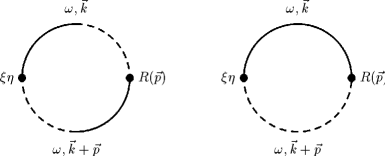
Figure 1: Feynman diagrams for calculating the coefficient $c_{1}$. The energy and momentum flow counter-clockwise around the loop.

References

- [1] M.H. Anderson et al., Science 269, 198 (1995); C.C. Bradley et al., Phys. Rev. Lett. 75, 1687 (1995); K.B. Davis et al., Phys. Rev. Lett. 75, 1969 (1995).
- [2] A.L. Fetter, Ann. Phys. (N.Y.) 70, 67 (1972).
- [3] V.V. Goldman, I.F. Silvera and A.J. Leggett, Phys. Rev. B 24, 2870 (1981).
- [4] D.A. Huse and E.D. Siggia, J. Low Temp. Phys. 46, 127 (1982).
- [5] A. Griffin, Phys. Rev. B 53, 9341 (1996).
- [6] P.C. Hohenberg and P.C. Martin, Ann. Phys. (N.Y.) 34, 291 (1965).
- [7] E. Braaten and A. Nieto, Phys. Rev. B 56, 14745 (1997).
- [8] D.M. Stamper-Kurn et al., Phys. Rev. Lett. 80, 2027 (1998).
- [9] S. Inouye et al., Nature 392, 151 (1998).
- [10] G. Baym and C.J. Pethick, Phys. Rev. Lett. 76, 6 (1996).
- [11] E. Braaten and A. Nieto, Phys. Rev. B 55, 8090 (1997).
- [12] E. Braaten and A. Nieto, cond-mat/9712041.
- [13] T. Haugset, H. Haugerud, and F. Ravndal, Ann. Phys. 226, 27 (1998).
- [14] V.N. Popov, Functional Integrals and Collective Excitations, Chapter 7 (Cambridge University Press, 1987).
- [15] S. Stringari, Phys. Rev. Lett. 77, 2360 (1996).
- [16] E. Timmermans, P. Tommasini, and K. Huang, Phys. Rev. A 55, 3645 (1997).
- [17] P.O. Fedichev and G.V. Shlyapnikov, cond-mat/9805015.