Wandering of a contact-line at thermal equilibrium

Abstract

We reconsider the problem of the solid-liquid-vapour contact-line on a disordered substrate, in the collective pinning regime. We go beyond scaling arguments and perform an analytic computation, through the replica variational method, of the fluctuations of the line. We show how gravity effects must be included for a proper quantitative comparison with available experimental data of the wetting of liquid helium on a caesium substrate. The theoretical result is in good agreement with experimental findings for this case.

1 Introduction

When a liquid partially wets a solid, the liquid-vapour interface terminates on the solid, at the contact line. If the solid surface is smooth, then at equilibrium, we expect no distortions of the contact line, and the Young’s relation [1] giving the contact angle in terms of the interfacial tensions holds, that is

$$\gamma_{sv}-\gamma_{sl}=\gamma\cos(\theta_{eq})$$ (1)

where $\gamma=\gamma_{lv}$, and $\theta_{eq}$ is the equilibrium mean contact angle.

We consider a case where the substrate is weakly heterogeneous and where the heterogeneities are “wettable” defects, leading to a space dependance of the interfacial tensions $\gamma_{sv}$ and $\gamma_{sl}$. Favoured configurations are those where the liquid can spread on a maximum number of defects. We thus expect distortions of the contact line which tends to be pinned by the defects. Moreover, the energy due to the liquid-vapour interface induces an elastic energy of the line. The competition between the elastic energy and the pinning due to the disorder gives rise to a non trivial wandering of the line, a typical example of the general problem of manifolds in random media [2, 3]. The case of the contact line is of special interest for several reasons. There exists by now good experimental data for the correlations which characterize the wandering of the line [4]. On the theoretical side, the problem presents two specific features. The elasticity of the line is non local. The pinning energy due to the surface heterogeneities is, up to a constant, a sum of local energy contributions due to the wetted defects. It has therefore non-local correlations which are of the “random field” type in the usual nomenclature of manifolds in random media.

In this paper we will consider the case of collective pinning where the strength of the individual pinning sites is small, but pinning occurs due to a collective effect. This seems to be the relevant situation for the experiments. The case of strong pinning by individual impurities was studied by Joanny and De Gennes [5]. Collective pinning is a particularly interesting phenomenon since the balance between the elastic energy and the pinning one results in the existence of a special length scale $\xi$, first discussed by Larkin in the context of vortex lines in superconductors [6]. This Larkin length is such that the lateral wandering of a line, thermalized at low temperatures, on length scales smaller than $\xi$, are less than the correlation length $\Delta$ of the disorder (range of the impurities), while beyond $\xi$ the lateral fluctuations become larger than $\Delta$ and the line probes different impurities. The Larkin length scale diverges in the limit where the strength of disorder goes to zero. At zero temperature, the line has a single equilibrium position when its length is smaller than $\xi$, while metastable states appear only for lengths larger than $\xi$. Therefore one can think of the contact line, qualitatively, as an object which is rigid on small length scales (less than $\xi$), and fluctuates on larger length scales. A third length scale which is relevant for the discussion is the capillary length $L_{c}$, which is the length scale beyond which effects due to gravity become important: the line then becomes “flat” in the sense that its fluctuations do not grow any longer with the distance.

The collective pinning of the contact line was first addressed by Vannimenus and Pomeau [7]. They considered the case of very weak disorder in which the Larkin length $\xi$ is larger than the capillary length. So their analysis only probes the “Larkin regime” of length scales less than $\xi$, in which there exist only very few metastable states. A more complete qualitative picture, making clear the role of $\xi$, can be obtained by some scaling arguments originally developped for some related problems by Larkin [6] and Imry-Ma [8]. For the case of the contact line, these arguments were introduced by Huse [10] and developped by De Gennes [1] and by Joanny and Robbins [9]. They lead to interesting predictions concerning the lateral fluctuations of the line: these should grow like the distance to the power $1/2$ on length scales less than $\xi$, and to the power $1/3$ on larger distances on length scales between $\xi$ and $L_{c}$. More recently, Kardar and Ertaz [11] have performed a dynamic renormalisation group calculation for the contact-line at zero temperature, subject to a uniform pulling force and also find a roughness exponent $1/3$. These scaling laws have been confirmed in recent experiments on the wetting of helium on a caesium substrate [4], confirming the validity of the collective pinning picture in this case.

The aim of our paper is to go beyond the scaling analysis and provide a quantitative computation of the correlation function of the line. We use the replica method together with a gaussian variational approximation, with replica symmetry breaking [12]. This approach, which is exact in the limit of large dimensions, is known to give good results even for one dimensional systems as this one [13, 14, 15]. It confirms the scaling exponents derived before, but also provides the prefactors and a full description of the crossover between the two regimes around the Larkin length.

The paper is organised as follows: We introduce the model in section (2). In section (3), we present for completeness a scaling argument which gives the roughness exponents, and we obtain an expression for the Larkin length by a perturbative approach. In section (4), we present the replica calculation and compute within a variational approximation the full correlation function in the limit of low temperatures, first neglecting gravity effects, and then including them. In section (5), we compare our theoretical prediction with experimental data.

2 The model

Figure 1: Sketch of the experimental set up

Consider a situation given by figure (1), where the liquid wets an impure substrate which is slightly inclined with respect to the horizontal. We denote by $(x,y)$ the space co-ordinates of the substrate. The excess energy per unit area due to pinning is given by

$$e(x,y)=\gamma_{sl}(x,y)-\gamma_{sv}(x,y)-\overline{\gamma_{sl}(x,y)-\gamma_{sv}(x,y)}$$ (2)

resulting in a total pinning energy

$$\int_{0}^{L}dx\int_{0}^{\Phi(x)}dy\ e(x,y)$$ (3)

where $\Phi(x)$ is the height of the the contact line at the abscissa $x$ (overhangs are neglected), and $L$ the width of the substrate. As for the pinning energy per unit area or force per unit length $e(x,y)$, we shall suppose that it is gaussian distributed, which is the case if it results from a large number of microscopic interactions, and that it has local correlations on length scales of order $\Delta$. Specifically, we choose

$$\overline{e(x,y)e(x^{\prime},y^{\prime})}=\frac{W}{\Delta^{2}}\delta(x-x^{\prime})C\biggl{(}\displaystyle\biggl{|}\frac{y-y^{\prime}}{\Delta}\biggr{|}\biggr{)}$$ (4)

where the correlation function $C(r)$ is normalised to $C(0)=1$ and $C^{\prime\prime}(0)=-1$, and decreases fast enough to zero for $r\gg 1$. The asymmetry introduced in (4) between the two directions $x$ and $y$ is for computational convenience. In most physical situations,the distribution of disorder should be isotropic in the $x-y$ plane, leading to a correlation in the $x$ direction on length scales of order $\Delta$. As we shall explain below, we have found that this correlation has only small effects, which exist only on very short distances and are not relevant experimentally. As for the shape of the function $C(r)$, we shall first use for simplicity

$$C(r)=f(r)=\exp(-r^{2}/2)\ ,$$ (5)

and we shall later comment on the modification of our result for more general correlations.

We must also add to the random potential term, a capillary energy term, which, if we neglect gravity and suppose that the slope of the liquid-vapour interface varies smoothly, is given by

$$E_{\rm cap}=\frac{c}{2}\displaystyle\int_{\frac{2\pi}{L}\leq|k|\leq\frac{2\pi}{\Delta}}\frac{dk}{2\pi}|k||\Phi(k)|^{2}$$ (6)

with $c=\displaystyle\frac{\gamma\sin^{2}\theta_{eq}}{2}$, $\theta_{eq}$ being the average equilibrium contact angle[9].

The final hamiltonian is thus

$$H=\frac{c}{2}\displaystyle\int_{\frac{2\pi}{L}\leq|k|\leq\frac{2\pi}{\Delta}}\frac{dk}{2\pi}|k|\ |\Phi(k)|^{2}+\int_{0}^{L}dx\ V(x,\Phi(x))$$ (7)

where $\displaystyle V(x,\Phi)=\int_{0}^{\Phi(x)}dy\ e(x,y)$. As a sum of independent gaussian variables, $V(x,\Phi)$ is gaussian distributed, and up to a uniform arbitrary random shift we can choose:

$$\overline{V(x,\Phi)V(x^{\prime},\Phi^{\prime})}=-W\delta(x-x^{\prime})f\biggl{(}\biggl{(}\frac{\Phi-\Phi^{\prime}}{\Delta}\biggr{)}^{2}\biggr{)}$$ (8)

where $f(u)$ is a function which grows as $\sqrt{|u|}$ for large $|u|$. Its precise form depends on the correlation function $C$ of the energy per unit area, and is given in the simple case (5) by

$$f(u^{2})=\displaystyle|u|\int_{0}^{|u|}dv\ e^{-v^{2}/2}-(1-e^{-u^{2}/2})$$ (9)

This model provides a good description of the problem of a contact line on a disordered substrate under the following hypotheses:

$\bullet$ The slope of the liquid-vapour interface is everywhere small.

$\bullet$ The length of the contact line is small compared with the capillary length, so that one can neglect gravity.

$\bullet$ The defects in the substrate are weak and give rise to collective pinning.

The main part of our work will be dedicated to the analytical study of this simplified model. We shall then examine the corrections due to gravity, to more general correlations of the disorder, and to the correlations in the $x$ direction. The quantity which is measured experimentally and which we shall compute is the correlation function of the position of the line:

$$\overline{\langle(\Phi(x)-\Phi(y))^{2}\rangle}$$ (10)

where thermal averages are denoted by angular brackets and the average over disorder by an overbar. As we shall see, in different length regimes, this correlation increases as a power law, which defines locally the wandering exponent $\zeta$ from:

$$\overline{\langle(\Phi(x)-\Phi(x))^{2}\rangle}\sim|x-x^{\prime}|^{2\zeta}\ .$$ (11)

3 Perturbation theory and scaling arguments

For completeness we rederive in this section an expression for the Larkin length by perturbation theory, and review the scaling derivation of the roughness exponents.

3.1 The Larkin length

On a sufficiently small length scale, we can assume that the difference in heights between any two points is small compared with the correlation length $\Delta$ of the potential. We can thus linearize the potential term [6] such that $V(x,\Phi(x))\simeq V(x,0)-e(x)\Phi(x)$. This leads to a random force problem with a force correlation function $\displaystyle\overline{e(x)e(x^{\prime})}=\frac{W}{\Delta^{2}}\delta(x-x^{\prime})$. Rewriting the hamiltonian as:

$$H=\displaystyle\frac{c}{2}\displaystyle\int\frac{dk}{2\pi}\ |k|\ \biggl{|}\Phi(k)-\frac{e(k)}{c|k|}\biggr{|}^{2}-\frac{1}{2c}\displaystyle\int\frac{dk}{2\pi}\ \frac{|e(k)|^{2}}{|k|}$$ (12)

we get for $T\rightarrow 0$ and $\Delta\ll|x-x^{\prime}|\ll L$,

$$\overline{<(\Phi(x)-\Phi(x^{\prime}))^{2}>}=\frac{2W}{c^{2}\Delta^{2}}\int\ \frac{dk}{2\pi}\frac{(1-\cos(k(x-x^{\prime})))}{k^{2}}=\frac{W}{c^{2}\Delta^{2}}|x-x^{\prime}|$$ (13)

The wandering exponent in the Larkin regime is given by $\zeta=1/2$. The linear approximation is no longer valid when $|\Phi(x)-\Phi(x^{\prime})|$ becomes of the order $\Delta$. Typically $|x-x^{\prime}|$ is then of order $\displaystyle\xi=\frac{c^{2}\Delta^{4}}{W}$, where $\xi$ is the so called Larkin length.

3.2 Roughness exponent for large fluctuations

On length scales larger than $\xi$, the fluctuations of the line are greater than the correlation length $\Delta$ and perturbation theory breaks down. One can estimate the wandering exponent by a simple scaling argument as follows [12]. The hamiltonian is given by (7) and we can no longer linearize the potential term in (7).

We consider the scale transformation, $x\rightarrow lx$, $\Phi(x)\rightarrow l^{\zeta}\Phi(x)$, $V(x,\Phi(x))\rightarrow l^{\lambda}V(x,\Phi(x))$. Imposing that the two terms in the hamitonian scale in the same way and that the potential term keeps the same statistics after rescaling, we have

$$\lambda=2\zeta-1\quad\mbox{and}\quad 2\lambda=-1+\zeta$$ (14)

and so $\zeta=1/3$. Note that this is less than the value $1/2$ obtained in the Larkin regime. On a still larger length scale (larger than the capillary length), we expect the line to be flat and $\zeta=0$.

This exponent can be recovered by the following Imry-Ma argument [8, 10, 1, 9]. On a scale $L$, the line fluctuates over a distance $\Phi$. The elastic energy contribution then scales as $c{\Phi}^{2}$. As for the pinning energy, since it is a sum of independant gaussian variables, it scales as $\displaystyle\sqrt{W\Delta}\sqrt{\frac{L\Phi}{\Delta^{2}}}$, where $\sqrt{W\Delta}$ is a measure of the pinning energy on an area $\Delta^{2}$ and $\displaystyle\frac{L\Phi}{\Delta^{2}}$ an order of magnitude of the number of such pinning sites. Minimising the total energy $\displaystyle c{\Phi}^{2}-\sqrt{W\Delta}\sqrt{\frac{L\Phi}{\Delta^{2}}}$ with respect to $\Phi$, we get $\displaystyle\Phi\simeq\Delta\biggl{(}\frac{L}{\xi}\biggr{)}^{1/3}$ with $\displaystyle\xi\sim\frac{c^{2}\Delta^{4}}{W}$.

4 The replica computation

4.1 Computation of the free energy

We now turn to a microscopic computation of the free energy $F=-T\ln Z$. Since the free energy is a self averaging quantity, the typical free energy is equal to the average of $F$ over the disorder. We compute it from the replica method with an analytic continuation of $\overline{Z^{n}}$, for $n\rightarrow 0$ [16]. The $n^{th}$ power of the partition function

$$Z^{n}=\int\prod_{a=1}^{n}d[\Phi_{a}]\ \exp\left\{-\frac{\beta c}{2}\int\frac{dk}{2\pi}\sum_{a}|k||\Phi_{a}(k)|^{2}-\beta\sum_{a}\int_{0}^{L}dx\ V(x,\Phi_{a}(x))\right\}$$ (15)

gives after averaging over the disorder

$$\overline{Z^{n}}=\int\prod_{a=1}^{n}d[\Phi_{a}]\ \exp\left\{-\beta{\cal H}_{n}[\Phi_{a}]\right\}$$ (16)

where

$${\cal H}_{n}=\frac{c}{2}\int\frac{dk}{2\pi}\sum_{a}|k||\Phi_{a}(k)|^{2}+\frac{\beta W}{2}\sum_{a,b}\int_{0}^{L}dx\ f\biggl{(}\biggl{(}\frac{\Phi_{a}(x)-\Phi_{b}(x)}{\Delta}\biggr{)}^{2}\biggr{)}$$ (17)

We note that the expression of the free energy is invariant with respect to a translation of the centre of mass of the line $\Phi_{CM}=\frac{1}{L}\int_{0}^{L}dx\ \Phi(x)=\frac{1}{L}\Phi(k=0)$. We can fix the centre of mass so that there is no integration on the $k=0$ mode. The partition function $\overline{Z^{n}}$ cannot be computed directly. Following [12], we perform a variational calculation based on the variational hamiltonian

$${\cal H}_{o}=\int\frac{dk}{2\pi}\sum_{a,b=1}^{n}\Phi_{a}(-k)G_{ab}^{-1}(k)\Phi_{b}(k)$$ (18)

where $G^{-1}$ is a hierarchical Parisi matrix.

The variational free energy

$${\cal F}=\frac{-1}{\beta n}\ln Z_{o}+\frac{1}{n}<{\cal H}_{n}-{\cal H}_{o}>_{o}$$ (19)

gives up to a constant term,

$$\frac{{\cal F}}{L}=\lim_{n\rightarrow 0}\ \frac{1}{n}\biggl{[}\frac{-1}{2\beta}\int\frac{dk}{2\pi}\mbox{Tr}_{a}\ln G+\frac{c}{2\beta}\int\frac{dk}{2\pi}|k|\sum_{a}G_{aa}(k)+\frac{\beta W}{2}\sum_{a\not=b}{\hat{f}}\biggl{(}\frac{B_{ab}}{\Delta^{2}}\biggr{)}\biggr{]}$$ (20)

where

$$\hat{f}(z)\ =\int_{-\infty}^{\infty}\ \frac{du}{\sqrt{2\pi}}f(u^{2}z)\ e^{-u^{2}/2}\ =\sqrt{1+z}-1$$ (21)

and

$$B_{ab}=\frac{1}{\beta}\int\frac{dk}{2\pi}\ (G_{aa}(k)+G_{bb}(k)-2G_{ab}(k))$$ (22)

The optimal free energy is obtained for a matrix $G$ verifying the stationarity conditions $\displaystyle\frac{\partial{\cal F}}{\partial G_{ab}}=0$, which read

$$\begin{array}[]{l}G_{ab}^{-1}=\displaystyle\frac{-2\beta W}{\Delta^{2}}{\hat{f}^{\prime}}\biggl{(}\frac{B_{ab}}{\Delta^{2}}\biggr{)}\quad\mbox{for}\quad a\not=b\\ \\ \displaystyle\sum_{b}G_{ab}^{-1}=c|k|\end{array}$$ (23)

More details on this approach can be found in [12, 16, 17].

4.2 The replica symmetry breaking solution

To solve equations (23), we suppose that the matrix $G$ has a hierarchical replica symmetry breaking stucture à la Parisi. We can write $G_{ab}^{-1}=(c|k|-{\tilde{\sigma}})\delta_{ab}-\sigma_{ab}$. $G^{-1}$ is thus parametrised by a diagonal part $c|k|-{\tilde{\sigma}}$, and a function $\sigma(u)$ defined on the interval $[0,1]$ . The optimisation equations for $G$ can then be written as:

$$\sigma(u)=\frac{2\beta W}{\Delta^{2}}{\hat{f}^{\prime}}\biggl{(}\frac{B(u)}{\Delta^{2}}\biggr{)}$$ (24)

with

$$B(u)=\frac{2}{\beta}\int\frac{dk}{2\pi}({\tilde{g}(k)}-g(k,u))$$ (25)

The solution to these equations is described in appendix A. It is best written in terms of the function

$$[\sigma](u)=u\sigma(u)-\int_{0}^{u}\ dv\ \sigma(v)$$ (26)

which is given by

$$\begin{array}[]{l}[\sigma](u)=\displaystyle\frac{W}{\pi c\Delta^{4}}\displaystyle\biggl{(}\frac{u}{u_{c}}\biggr{)}^{3/2}\quad\mbox{for}\quad u\leq u_{c}\par\\ \\ [\sigma](u)=\displaystyle\frac{W}{\pi c\Delta^{4}}\quad\mbox{for}\quad u\geq u_{c}\end{array}$$ (27)

We shall give the value of the breakpoint $u_{c}$ in the (experimentally relevant) limit of low temperatures. Defining

$$T_{c}=\pi c\frac{\Delta^{2}}{3}\ ,$$ (28)

we get $u_{c}\simeq T/T_{c}$. From the expression

$$G_{aa}(k)=\frac{1}{c|k|}\biggl{[}1+\int_{0}^{1}\frac{du}{u^{2}}\frac{[\sigma](u)}{[\sigma](u)+c|k|}\biggr{]}$$ (29)

we obtain in the regime $\Delta\ll|x-x^{\prime}|\ll L$

$$\sqrt{\overline{<(\Phi(x)-\Phi(x^{\prime}))^{2}>}}=\Delta{\cal H}\biggl{(}\frac{x-x^{\prime}}{\xi}\biggr{)}$$ (30)

where

$${\cal H}^{2}(x)=\frac{4}{3}\biggl{(}\frac{x}{\pi}\biggr{)}^{2/3}\int_{0}^{\infty}dk\frac{(1-\cos(k))}{k^{5/3}}\int_{0}^{(x/{\pi k})^{1/3}}\frac{dw}{w^{3}+1}\ +\frac{2x}{3\pi}\int_{0}^{\infty}dk\frac{(1-\cos(k))}{k(x/{\pi}+k)}$$ (31)

and $\displaystyle\xi=\displaystyle\frac{c^{2}\Delta^{4}}{W}$.

The function ${\cal H}$ is the analytical prediction in the regime where gravity effects can be neglected. It is plotted in figure 2 and has the following asymptotic behaviour. For small $x$, ${\cal H}(x)\simeq\sqrt{|x|}$ and for large $x$, ${\cal H}(x)\simeq 1.14|x|^{1/3}$. Therefore the predictions in the various scaling regimes, including prefactors, is as follows.

When $|x-x^{\prime}|\ll\xi$, (Larkin regime):

$$\sqrt{\overline{<(\Phi(x)-\Phi(x^{\prime}))^{2}>}}\simeq\Delta\left|\frac{x-x^{\prime}}{\xi}\right|^{1/2}$$ (32)

When $|x-x^{\prime}|\gg\xi$, (random manifold regime):

$$\sqrt{\overline{<(\Phi(x)-\Phi(x^{\prime}))^{2}>}}\simeq 1.14\Delta\left|\frac{x-x^{\prime}}{\xi}\right|^{1/3}$$ (33)

Before turning to the comparison with the experiment, we first compute various correction factors to this formula.

Figure 2: The theoretical predictions for the rescaled height correlations. From top to bottom, the curve ${\cal H}(x)$ (30) where gravity is neglected ($\lambda=\pi\xi/L_{c}=0$), and the curves ${\cal H}_{g}(x,\lambda)$ for values of $\lambda$ such that $\lambda=0.1,0.2,0.4,0.6,0.8$. Notice the need to have a very small ratio of Larkin length to capillary length in order for the zero gravity result to be good.

4.3 A more general form of the disorder

We show that even in the more general case where we only impose that the correlation function of the potential has the asymptotic behaviour $f(|u|)\sim\sqrt{|u|}$ for large $|u|$, the height correlation function can be put in the form

$$\sqrt{\overline{<(\Phi(x)-\Phi(x^{\prime}))^{2}>}}=\Delta{\cal G}\biggl{(}\frac{x-x^{\prime}}{\xi}\biggr{)}$$ (34)

in the limit $T\rightarrow 0$, and for $\Delta\ll|x-x^{\prime}|\ll L$. The derivation of ${\cal G}$, for an arbitrary correlation function $f$, is given in appendix B.

4.4 Effect of the cut-off $\Delta$ at small $x$

Coarse-graining the force in the $x$ direction on scales of order $\Delta$ leads to a discretized (in $x$) version of (4), which is equivalent to the form which we use, but with a cut off of order $\Delta$ at small $x$. On scales comparable to $\Delta$, there are thus corrections to equation (31) due to this cutoff, which are easily computed. When we take into account the cut-off $\Delta$, the correlation function ${\cal H}$ becomes

$${\cal H}_{1}^{2}(x,\nu)=\frac{4}{3}\biggl{(}\frac{x}{\pi}\biggr{)}^{2/3}\int_{0}^{2\pi\nu x}\frac{dk}{k^{5/3}}(1-\cos(k))\int_{0}^{(x/{\pi k})^{1/3}}\frac{dw}{w^{3}+1}\ +\frac{2x}{3\pi}\int_{0}^{2\pi\nu x}\frac{dk}{k(x/{\pi}+k)}(1-\cos(k))$$ (35)

where $\displaystyle\nu=\frac{\xi}{\Delta}$. The effect of the cut-off is to shift slightly downwards the theoretical curve, especially in the region of small $x$.

4.5 Effect of gravity

In the geometry considered, the effective capillary length is given by $\displaystyle\sqrt{\frac{\gamma}{\rho g\sin\alpha}}$, where $\alpha$ is the tilt angle of the substrate with respect to to horizontal [4]. To take into account gravity we must replace the kernel $|k|$ in the hamiltonian (7) by $\sqrt{k^{2}+1/L_{c}^{2}}$, where $L_{c}$ is the capillary length. Generalising the previous calculation we have computed the corrections due to gravity. The fluctuation of the line at distance $x$ now depends on two parameters, $x/\xi$ and $\lambda=\pi\xi/L_{c}$. The computation done in appendix C expresses $[\sigma](u)$ in the terms of an inverse function ${\cal I}^{-1}$. When the Larkin length is sufficiently small compared with the capillary length, that is when $\xi$ is less than approximately $0.5L_{c}$, we have in the limit where $T\ll T_{c}$

$$\begin{array}[]{l}[\sigma](u)=0\quad\mbox{for}\quad u\leq u_{1}\par\\ \\ [\sigma](u)=\displaystyle\mu c\ {\cal I}^{-1}\biggl{(}\frac{L_{c}}{\pi\xi}\displaystyle\biggl{(}\frac{u}{u_{c}}\biggr{)}^{3/2}\biggr{)}\quad\mbox{for}\quad u_{1}\leq u\leq u^{\prime}_{c}\par\\ \\ [\sigma](u)=\displaystyle\mu c\ {\cal I}^{-1}\biggl{(}\frac{L_{c}}{\pi\xi}\biggl{(}\frac{u^{\prime}_{c}}{u_{c}}\biggr{)}^{3/2}\biggr{)}\quad\mbox{for}\quad u\geq u^{\prime}_{c}\par\\ \\ \mbox{with}\quad\displaystyle u_{1}=u_{c}\biggl{(}\frac{\pi\xi}{L_{c}}{\cal I}(0)\biggr{)}^{2/3}\quad\mbox{and}\quad u_{c}\simeq\displaystyle\frac{T}{T_{c}}\end{array}$$ (36)

As for $u^{\prime}_{c}$, it is slightly larger than $u_{c}$ and also of order $\displaystyle\frac{T}{T_{c}}$. When the capillary length goes to infinity $u_{1}$ tends towards $0$ and $u^{\prime}_{c}$ towards $u_{c}$. The function ${\cal I}(x)$ is given by

$${\cal I}(x)=\displaystyle\biggl{(}\int_{0}^{\infty}\frac{dk}{(\sqrt{q^{2}+1}+x)^{2}}\biggr{)}^{2}\biggl{(}2\int_{0}^{\infty}\frac{dk}{(\sqrt{q^{2}+1}+x)^{3}}\biggr{)}^{-3/2}$$ (37)

and for large $x$, ${\cal I}(x)\simeq x$. This asymptotic behaviour ensures that we do recover the results of section (5) when $\mu$ goes to zero. The correlation is now given by

$$\sqrt{\overline{<(\Phi(x)-\Phi(x^{\prime}))^{2}>}}=\Delta{\cal H}_{g}\biggl{(}\frac{x-x^{\prime}}{\xi},\frac{\pi\xi}{L_{c}}\biggr{)}$$ (38)

where

$$\begin{array}[]{ll}{\cal H}^{2}_{g}(x,\lambda)=&\displaystyle\frac{4}{3}\int_{0}^{\infty}dk\frac{(1-\cos(kx/\pi)}{\sqrt{k^{2}+\lambda^{2}}}\displaystyle\int_{(\lambda{\cal I}(0))^{1/3}}^{(u^{\prime}_{c}/u_{c})^{1/2}}\frac{dw}{w^{3}}\frac{\lambda{\cal I}^{-1}(w^{3}/\lambda)}{\lambda{\cal I}^{-1}(w^{3}/\lambda)+\sqrt{k^{2}+\lambda^{2}}}\par\\ \\ &+\displaystyle\frac{2}{3}\frac{u_{c}}{u^{\prime}_{c}}\int_{0}^{\infty}dk\ \frac{(1-\cos(kx/\pi)}{\sqrt{k^{2}+\lambda^{2}}}\frac{\lambda{\cal I}^{-1}(1/\lambda)}{\lambda{\cal I}^{-1}(1/\lambda)+\sqrt{k^{2}+\lambda^{2}}}\end{array}$$ (39)

The asymptotic behaviour of ${\cal H}_{g}$ is different from that of $\cal H$. For small $x$

$${\cal H}^{2}_{g}(x,\lambda)\simeq x\biggl{\{}\frac{2}{3}\int_{(\lambda{\cal I}(0))^{1/3}}^{(u^{\prime}_{c}/u_{c})^{1/2}}dw\ \frac{\lambda}{w^{3}}{\cal I}^{-1}(w^{3}/\lambda)+\frac{u_{c}}{3u^{\prime}_{c}}\lambda{\cal I}^{-1}(1/\lambda)\biggl{\}}$$ (40)

and for large $x,{\cal H}_{g}(x,\lambda)$ tends towards a constant depending on $\lambda$.

From the previous equations we can see that gravity has a significant effect when $\displaystyle\lambda=\frac{\pi\xi}{L_{c}}$ becomes of order $1$, where $\xi$ is the Larkin length and $L_{c}$ the capillary length. Moreover we can also note that the correction for small $\lambda$ to the case without gravity is of order $\lambda^{1/3}$. The limit $\lambda$ going to $0$ is thus a rather slow one. This is illustrated in figure (2).

5 Comparison with experiment

5.1 The experimental set up

We have fitted the data from experiments carried out by C.Guthmann and E.Rolley [4] with our theoretical curve. The experiments study the wetting properties of liquid helium 4 on caesium below the wetting transition temperature which is about $2K$. Above that temperature caesium is wetted by helium. In the experiments carried out by Guthmann and Rolley the substrate consists of caesium deposited on a gold mirror which is slightly inclined with respect to the horizontal (see figure 1). The wetted defects are small areas on the substrate where the caesium has been oxydised. The experiments are carried out on a range of temperatures going from about $1K$ to $2K$. There is a constant inflow of helium at the bottom of the helium reservoir to maintain the contact angle to its maximum value $\theta_{a}$, the advancing angle, which is in general different from the equilibrium contact angle $\theta_{eq}$ (see figure 1). This is necessary because otherwise, the liquid would recede and the contact angle would shrink to zero due to strong hysteresis. Height correlations are calculated from snapshots of the advancing line when it is pinned. The incoming helium is regulated to ensure that the line moves with a small velocity and so we can probably suppose can we are just at the limit of depinning.

The predicted order of magnitude of $T_{c}$ given by (28) is $\displaystyle\frac{\pi c\Delta^{2}}{3}=\displaystyle\frac{\pi\gamma\sin^{2}(\theta_{eq})\Delta^{2}}{6}$. The size of the impurities can be measured experimentally and is of the order of $20\mu m$. We thus expect the correlation length to be a few times this size. Its precise value depends on the details of the disorder. For temperatures not too close to transition temperature, $\theta_{eq}\sim 20$ degrees, and $\gamma\sim 10^{19}Km^{-2}$. This leads to a typical estimate $T_{c}\sim 10^{8}K$, in the experimental conditions of [4]. Therefore $T/T_{c}$ is of order $10^{-8}$ and the system is effectively at low temperatures, justifying the low temperature limit in our computations.

5.2 Comparison between experimental data and the theory neglecting gravity

We consider experimental data for height correlations ${\cal H}_{exp}(x)=\sqrt{\overline{<(\Phi(x)-\Phi(0))^{2}>}}$ for temperatures $T=1.72,1.8,1.9,1.93K$. The equilibrium angle $\theta_{eq}$, the liquid-vapour interfacial tension $\gamma$ and the “potential stength” $W$ depend on the temperature, and so the various experimental curves correspond a-priori to different values of the Larkin length. Instead, the correlation length $\Delta$ which depends only on the substrate, is expected to remain constant. We have thus fitted the experimental curves to the theoretical prediction in the absence of gravity (30) and (38), with the same $\Delta$ but different $\xi$’s.

We proceed as follows. We first minimise the error function

$${\cal E}=\displaystyle\frac{1}{\displaystyle\sum_{j}N_{j}}\sum_{j=1}^{4}\sum_{i=1}^{N_{j}}\biggl{(}\Delta{\cal H}(x_{i}/\xi_{j})-{\cal H}_{exp}(x_{i})\biggl{)}^{2}$$ (41)

with respect to $\Delta$ and $\xi_{j}$ for $j\in[1,4]$, where $j$ denotes a given experimental curve at the temperature $T_{j}$, $x_{i}$ the experimental points, $N_{j}$ the number of points of curve $j$, and $\xi_{j}$ the correlation length at temperature $T_{j}$. This procedure yields $\Delta\simeq 18\mu m$ and ${\cal E}\simeq 0.3\mu m^{2}$.

Figure 3: The experimental data for the fluctuation of the line as a function of the distance (circles). From top to bottom, the temperatures are $1.93K$, $1.9K$, $1.8K$ and $1.72K$. The full curves are the theoretical predictions in absence of gravity (30), using the values of Larkin lengths shown in table $1$.

In figure (3), we show the four experimental curves, together with the corresponding theoretical fit $\Delta{\cal H}(x/\xi_{j})$. The values of the Larkin lengths $\xi_{j}$ are given in table $1$ below. The dependance of $\xi$ on the temperature is related to the variations of $W$, $\gamma$ and $\theta_{eq}$, which are not known well enough for a detailed comparison between theory and experiment. It should be noted that the determinations of $\Delta$ on the one hand, and the $\xi_{j}$ on the other hand, are strongly correlated. (To give an idea, with $\Delta=19\mu m$, $\xi_{1}=60\mu m$, $\xi_{2}=104\mu m$, $\xi_{3}=163\mu m$, $\xi_{4}=248\mu m$ the error (41) differs from the previous case by about only $10{\%}$). In the absence of detailed information on the experimental error, it is thus difficult to give an error bar on $\xi$. On the other hand, the ratios of the Larkin lengths in different experiments are much less sensitive to this correlation. They are given in table $1$ as well.

T(K)	1.72	1.8	1.9	1.93
$\xi$($\mu m$)	220	145	92	53
$\xi/\xi_{1}$	4.1	2.7	1.7	1

Table 1: Values of the Larkin length scale used in the fit to the experiment shown in figures (3,4).

Figure 4: Collapse plot of all the experimental data on fluctuations of the line at various temperatures onto the theoretical prediction neglecting gravity (30), using the values of Larkin lengths shown in table $1$.

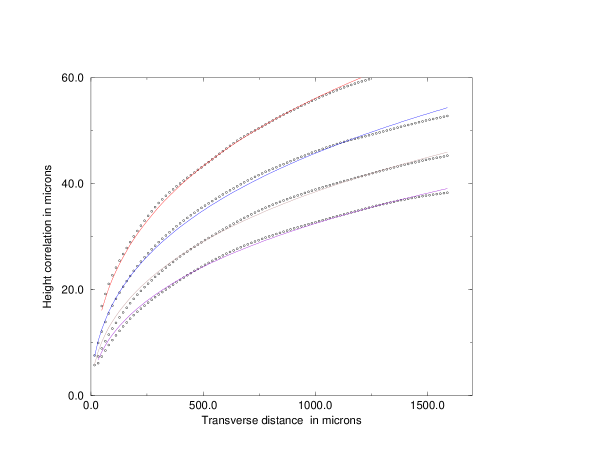
In figure (4), we show a collapse plot of all the experimental curve on the theoretical one with gaussian correlated disorder. We have rescaled each experimental curve by the corresponding $1/\xi$ in the $x$ direction and by $1/\Delta$ in the $y$ direction. This collapse gives several interesting results: the curves nearly collapse one onto the other, as expected from the general form (34). Furthermore it seems that the simplest correlation function that we have studied in most details (5) gives a reasonable fit to the data. We have also checked that the small $x$ cut-off discussed in section (4.4) is irrelevant. However there is also clearly, a systematic difference at large distances, which we shall now discuss.

5.3 Comparison between experimental data and the theory including gravity

In figure (4), we note that each of the rescaled experimental curves lies below the theoretical curve at large distances. Moreover the experimental curves have a slightly larger curvature than the rescaled theoretical curve. These are indications that gravity cannot be totally neglected. Indeed the effective capillary length in the experimental conditions is of the order of $2mm$, and experimentally the correlations are measured for distances up to about $1.5mm$, which is actually not small compared with the capillary length.

To check whether gravity has or not a significant effect, we have tried to fit the experiments with the full theoretical prediction including gravity (38). Encouraged by the results of the previous analysis, we keep to the case of a gaussian correlation function of the disorder given by (8),(9). We have carried out the same analysis as in the previous subsection, using as theoretical input ${\cal H}_{g}(x,\lambda)$ instead of ${\cal H}(x)$. The capillary length $L_{c}$ is not adjustable: it is calculated for the different temperatures from the experimental measurements of $\gamma$, and are given in table $2$. Therefore this new fit has the same number of adjustable parameters as the previous one. We now minimise the error function:

$${\cal E}_{g}=\displaystyle\frac{1}{\displaystyle\sum_{j}N_{j}}\sum_{j=1}^{4}\sum_{i=1}^{N_{j}}\biggl{(}\Delta{\cal H}_{g}(x_{i}/\xi_{j},\pi\xi_{j}/L_{c}^{j})-{\cal H}_{exp}(x_{i})\biggl{)}^{2}$$ (42)

As one could expect form the rather slow convergence of the theoretical curves ${\cal H}_{g}(x,\lambda)$ towards the gravity-free one ${\cal H}(x)={\cal H}_{g}(x,0)$ at small $\lambda$ (see figure 2), we find rather different values for the parameters. In this case, $\Delta\simeq 75\mu m$ and ${\cal E}_{g}\simeq 0.26\mu m^{2}$. The values of the Larkin lengths for the different temperatures are given in table $2$. We have the same problem of correlations between the determination of $\Delta$ and the Larkin lengths as before. The ratios of the Larkin lengths in different experiments are also given in table $2$.

T(K)	1.72	1.8	1.9	1.93
$L_{c}$ ($\mu m$)	1855	1838	1819	1823
$\xi$($\mu m$)	480	425	365	295
$\xi/\xi_{1}$	1.6	1.4	1.2	1

Table 2: Values of the experimental capillary lengths, and of the Larkin length scale used in the fit to the experiment shown in figure (5).

Figure 5: The experimental data for the fluctuation of the line as a function of the distance (circles). From top to bottom, the temperatures are $1.93K$, $1.9K$, $1.8K$ and $1.72K$. The full curves are the theoretical predictions in the presence of gravity (38), using the values of Larkin lengths shown in table $2$.

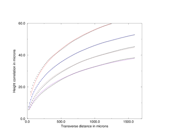In figure (5), we show the experimental curves together with the corresponding theoretical curve ${\cal H}_{g}(x,\lambda)$ including gravity. The fit is clearly better in this case since we have got rid of the systematic drift from the theory for large $x$. The exponents of the two experimentally observed regimes are correctly predicted by a theory without gravity, but to obtain the correct values of the correlation length and Larkin lengths it is necessary to take into account the effect of gravity.

6 Discussion and perspectives

Our analytic computation for the wandering of a contact line on a disordered substrate fits quite well the experimental data. We have shown that gravity effects are far from negligible and should be taken into account in order to extract the relevant parameters (which are basically the correlation length of the disorder as well as the Larkin length scale) from the experiments. Taking into account gravity in the theory clearly improves the fit to the data. Moreover, the theory including gravity will allow larger experimental length scales in the analysis.

A few comments about the validity of our computation are the following. First of all, we have used in most of our analysis a simple form for the correlation function of the disorder (5) which is not necessarily the correct one. It is true that some of our predictions are independant of this form, like for instance the existence of a scaling behaviour in absence of gravity. It is an experimental problem to have a better description of the pinning disorder at work, and we have shown that our computation can be extended to any type of correlation. The simplest one seems to give already a good account of the data. The variational method which has been used in this work is also an approximation. So far there is no other analytic quantitative method available, and it seems to work quite well, confirming previous evidence found in other problems [13, 14, 15].

A more interesting question concerns our assumption of an equilibrium situation. We have supposed that the line is in thermal equilibrium in order to write the usual partition function, and at the end of the calculation, we have taken the temperature to zero since, as we can see from the numerical values of the parameters, thermal fluctuations are irrelevant. In doing so, we retain only the states with the lowest energy. Experimentally the state of the line has no apparent reason to be a low temperature equilibrium state. It is difficult so far to characterize fully the metastable states that can be reached dynamically by the experimental procedure. They might have generically the same statistical properties as the ground state, this is actually under study ([18]). A less interesting but may be more realistic alternative, could be that because of gravity, the fluctuations of the line do not go much beyond the correlation length. So, even though we are out of the Larkin regime, we are not yet deep in the random manifold regime and there are thus not so many metastable states.

A purely dynamical computation could also be done. While the properties of the unpinned line have already been studied in [11], the dynamics of the pinned object could also be very interesting. If the correlation length of the disorder can be made much smaller, so that thermal fluctuation are no longer negligeable, we expect the onset of some ageing dynamics [19]. It will be interesting both to compute its properties and to measure them. In particular, this system might present a nice situation to measure the fluctuation-dissipation ratio in a system which has a full (continuous) replica symmetry breaking, offering a chance to measure directly the function $[\sigma](u)$.

Appendix A Computation of the function $[\sigma](u)$

We give in this appendix some details of the calculation of the function $[\sigma](u)$. We have from section (4),

$$\sigma(u)=\displaystyle\frac{2\beta W}{\Delta^{2}}{\hat{f}^{\prime}}\biggl{(}\frac{B(u)}{\Delta^{2}}\biggr{)}\\$$ (43)

where

$$B(u)=\frac{2}{\beta}\int\frac{dk}{2\pi}({\tilde{g}(k)}-g(k,u))$$ (44)

and from [12],

$${\tilde{g}(k)}-g(k,u)=\frac{1}{u(c|k|+[\sigma](u))}-\int_{u}^{1}\frac{dv}{v^{2}}\frac{1}{c|k|+[\sigma](v)}$$ (45)

Differentiating (43) gives

$$\sigma^{\prime}(u)=\displaystyle\frac{2\beta W}{\Delta^{4}}B^{\prime}(u){\hat{f}^{\prime\prime}}\biggl{(}\frac{B(u)}{\Delta^{2}}\biggr{)}\\$$ (46)

and replacing $B^{\prime}(u)$ in (46) by its expression

$$B^{\prime}(u)=\displaystyle-\frac{2}{\beta\pi c}\frac{\sigma^{\prime}(u)}{[\sigma](u)}$$ (47)

leads to

$$\begin{array}[]{c}\displaystyle\sigma^{\prime}(u)=0\quad\quad\mbox{or}\\ \\ \displaystyle 1=\displaystyle-\frac{4W}{\pi c\Delta^{4}}\frac{1}{[\sigma](u)}{\hat{f}}^{\prime\prime}\biggl{(}\frac{B(u)}{\Delta^{2}}\biggr{)}\end{array}$$ (48)

We express $\displaystyle\frac{B(u)}{\Delta^{2}}$ in terms of $[\sigma](u)$ by inverting the second equation of (48). This gives:

$${\hat{f}}^{\prime\prime-1}\biggl{(}\displaystyle-\frac{\pi c\Delta^{4}}{4W}[\sigma](u)\biggr{)}=\displaystyle\frac{B(u)}{\Delta^{2}}$$ (49)

Differentiating (49), and using expression (46) to express $B^{\prime}(u)$, and the fact that $[\sigma]^{\prime}(u)=u\sigma^{\prime}(u)$, we get

$$\frac{{\hat{f}}^{{}^{\prime\prime\prime}}}{{\hat{f}}^{{}^{\prime\prime}}}\biggl{(}\frac{B(u)}{\Delta^{2}}\biggr{)}=\displaystyle-\frac{\beta\pi c\Delta^{2}}{2}u=\displaystyle-\frac{3T_{c}}{2T}u$$ (50)

where

$${\hat{f}}^{\prime}(x)=\frac{1}{2\sqrt{1+x}}$$ (51)

From (50) and (51), we have

$$\frac{B(u)}{\Delta^{2}}=-1+\frac{3T}{\pi cu\Delta^{2}}=-1+\frac{T}{T_{c}}\frac{1}{u}$$ (52)

Multiplying both sides of equation (47) by $u$, and using (52) we get after integrating over u

$$[\sigma](u)=Au^{3/2}$$ (53)

The breakpoint $u_{c}$, above which the solutions to (52) and (53) are no longer valid is given by

$$B(u_{c})=\Delta^{2}\biggl{(}-1+\frac{T}{T_{c}}\frac{1}{u_{c}}\biggr{)}=\frac{2}{3}\frac{T}{T_{c}}\ln\biggl{(}1+\frac{2\pi c}{\Delta[\sigma](u_{c})}\biggr{)}$$ (54)

When $\displaystyle\frac{T}{T_{c}}$ goes to $0$, $u_{c}\simeq\displaystyle\frac{T}{T_{c}}$. Now since $B(u)$ tends to infinity when $u$ tends to $0$, we have $\sigma(0)=0$. For $u\geq u_{c}$, $B(u)=B(u_{c})$ and $[\sigma](u)=[\sigma](u_{c})$. To obtain $A$, we can differentiate (53) and compare the result with the expression for $\sigma^{\prime}(u)$. We find $\displaystyle A=\frac{W}{\pi c\Delta^{4}}\frac{1}{u_{c}^{3/2}}$. For $u\geq u_{c}$, $\sigma^{\prime}(u)=0$ and so $\displaystyle[\sigma](u)=[\sigma](u_{c})=\displaystyle\frac{W}{\pi c\Delta^{4}}$.

Appendix B General form of the correlation function for arbitrary disorder

In this appendix we derive the height correlation function for a more general form of the function $f$ appearing in the correlation function of the disorder (8). We only impose that $f(|u|)\sim\lambda\sqrt{|u|}$ for large $u$ where $\lambda$ is some constant, such that ${\hat{f}}(u)\sim\sqrt{|u|}$. We shall keep the same notations as in appendix A. In this more general case, equations (43),(47),(50) from appendix A are still valid. We define the function $h^{-1}$ for positive $x$ as

$$h^{-1}(x)=\displaystyle\frac{{\hat{f}}^{{}^{\prime\prime\prime}}(x)}{{\hat{f}}^{{}^{\prime\prime}}(x)}$$ (55)

where $\displaystyle h^{-1}(x)\sim-\frac{3}{2x}$ for large $x$. The asymptotic behaviour of $h(y)$ for small and negative $y$ is then $\displaystyle-\frac{3}{2y}$. We now express $B(u)$ in terms of $h$, from equations (50) and (55). This gives

$$B(u)=\Delta^{2}h\biggl{(}-\frac{\pi c\Delta^{2}}{2T}u\biggr{)}$$ (56)

Differentiating the previous equation (56) gives

$$B^{\prime}(u)=-\frac{\pi c\Delta^{4}}{2T}h^{\prime}\biggl{(}-\frac{\pi c\Delta^{2}}{2T}u\biggr{)}$$ (57)

which can be rewritten as

$$\frac{2T}{3T_{c}}\frac{d}{du}\log[\sigma](u)=wh^{\prime}(-w)$$ (58)

where $w=\displaystyle\frac{\pi c\Delta^{2}}{2T}u$. Integrating (58) gives

$$[\sigma](u)=\displaystyle[\sigma](\epsilon)\displaystyle\exp\displaystyle\int_{3\epsilon/2u_{c}}^{3u/2u_{c}}dw\ wh^{\prime}(-w)$$ (59)

For $\epsilon\leq u\ll u_{c}$, we can use the asymptotic form of $h$ in (59), which then reads

$$[\sigma](u)=[\sigma](\epsilon)\biggl{(}\frac{u}{\epsilon}\biggr{)}^{3/2}$$ (60)

Now for small $u$, equation (46) becomes in this case

$$\sigma^{\prime}(u)=\frac{3}{2}\frac{W}{\pi c\Delta^{4}}\biggl{(}\frac{T_{c}}{T}\biggr{)}^{3/2}\frac{1}{\sqrt{u}}$$ (61)

and so for small $u$, since $[\sigma](0)=0$, we get

$$[\sigma](u)=\frac{W}{\pi c\Delta^{4}}\biggl{(}\frac{u}{u_{c}}\biggr{)}^{3/2}$$ (62)

A comparison of this last expression with (60) gives

$$[\sigma](\epsilon)=\frac{W}{\pi c\Delta^{4}}\biggl{(}\frac{\epsilon}{u_{c}}\biggr{)}^{3/2}$$ (63)

Replacing this last expression in (59) and taking $\epsilon$ to zero leads to

$$[\sigma](u)=\frac{W}{\pi c\Delta^{4}}{\cal S}(u)$$ (64)

where

$${\cal S}(u)=\displaystyle\biggl{(}\frac{u}{u_{c}}\biggr{)}^{3/2}\exp\displaystyle{\int_{0}^{3u/2u_{c}}dw\ w\biggl{(}h^{\prime}(-w)-\frac{3}{2w^{2}}\biggr{)}}$$ (65)

For the sake of simplicity, we will suppose that in this case the break-point up to which expression (65) is valid, is also $u_{c}$ in the limit of low temperatures. This implicitely requires that $h(-3/2)=0$. Then for $u\geq u_{c}$

$${\cal S}(u)={\cal S}(u_{c})=\displaystyle\exp\displaystyle{\int_{0}^{3/2}dw\ w\biggl{(}h^{\prime}(-w)-\frac{3}{2w^{2}}\biggr{)}}$$ (66)

When ${\hat{f}^{\prime}}$ has the simple form (51), $\displaystyle h^{\prime}(-w)=\frac{3}{2w^{2}}$, and we recover the expression of $[\sigma](u)$ derived in appendix A.In the limit of low temperatures and for $\Delta\ll|x-x^{\prime}|\ll L$, the height correlation function is given by

$$\sqrt{\overline{<(\Phi(x)-\Phi(x^{\prime}))^{2}>}}=\Delta{\cal G}\biggl{(}\frac{x-x^{\prime}}{\xi}\biggr{)}$$ (67)

with

$$\begin{array}[]{ll}{\cal G}^{2}(x)=&\displaystyle\frac{4}{3}\biggl{(}\frac{x}{\pi}\biggr{)}^{2/3}\int_{0}^{\infty}dk\frac{(1-\cos(k))}{k^{5/3}}\int_{0}^{(x/{\pi k})^{1/3}}dv\ \displaystyle\frac{1}{v^{3}+\exp\displaystyle\biggl{(}-\int_{0}^{\frac{3v^{2}}{2}(\pi k/x)^{2/3}}dw\displaystyle\biggl{(}h^{\prime}(-w)-\frac{3}{2w^{2}}\biggr{)}\biggr{)}}\par\\ \\ &\quad\quad\quad\quad+\ \displaystyle\frac{2x}{3\pi}\int_{0}^{\infty}dk\displaystyle\frac{(1-\cos(k))}{k\biggl{(}x/{\pi}+k\exp\displaystyle\biggl{(}-\int_{0}^{3/2}dw\displaystyle\biggl{(}h^{\prime}(-w)-\frac{3}{2w^{2}}\biggr{)}\biggr{)}\biggr{)}}\end{array}$$ (68)

Appendix C Effect of gravity

In this appendix, we consider a specific case of the disorder given by equations (8) and (9). To take into account gravity, we must replace the kernel $|k|$ by $\sqrt{|k|^{2}+\mu^{2}}$, with $\displaystyle\mu=\frac{1}{L_{c}}$, where $L_{c}$ is the capillary length. The equations derived in appendix A are thus no longer valid. If $\sigma^{\prime}(u)$ is not zero then, equation (49) of appendix A becomes

$$\frac{B(u)}{\Delta^{2}}={\hat{f}}^{\prime\prime-1}\biggl{(}-\frac{\pi c\Delta^{4}}{4W}{\cal K}([\sigma](u))\biggl{)}$$ (69)

where

$${\cal K}(x)=c\mu\ g\biggl{(}\frac{x}{c\mu}\biggr{)}$$ (70)

with

$$\frac{1}{g(x)}=\int_{0}^{\infty}\frac{dk}{(\sqrt{k^{2}+1}+x)^{2}}$$ (71)

Differentiating (45) gives

$$B^{\prime}(u)=-\frac{2\sigma^{\prime}(u)}{\pi\beta c}\frac{1}{{\cal K}([\sigma](u))}$$ (72)

Differentiating (69), and using (46) and (51), we have

$$1+\frac{B(u)}{\Delta^{2}}=\frac{T}{T_{c}}\frac{1}{u{\cal K}([\sigma](u))}$$ (73)

Differentiating the previous expression (73), and using (72), we can express $[\sigma](u)$ as

$$\frac{{\cal K}([\sigma](u))}{({\cal K}^{\prime}([\sigma](u)))^{3/2}}=Au^{3/2}$$ (74)

where $A$ is a constant to be determined. Replacing in equation (46), $B^{\prime}(u)$ by its expression (69) and reexpressing (51) using (73) leads to

$$1=\frac{W}{\pi c\Delta^{4}}\frac{1}{u_{c}^{3/2}}\frac{(u{\cal K}^{\prime}([\sigma](u)))^{3/2}}{{\cal K}([\sigma](u))}$$ (75)

Comparing the previous expression with (74) gives

$$A=\frac{W}{\pi c\Delta^{4}}\frac{1}{u_{c}^{3/2}}$$ (76)

To express $[\sigma]$, it is convenient to introduce the function ${\cal I}$

$${\cal I}(x)=\displaystyle\frac{g(x)}{(g^{\prime}(x))^{3/2}}$$ (77)

which is strictly positive and increasing. ${\cal I}(0)\simeq 0.87$ and ${\cal I}(x)$ goes as $x$ when $x$ goes to infinity.

The inverse function ${\cal I}^{-1}$ is thus defined on the interval $[{\cal I}(0),\infty]$. Since $[\sigma](u)$ must be continuous and $[\sigma](0)=0$, the function $[\sigma]$ necessarily has a first plateau where $[\sigma](u)=0$ from $u=0$ up to a value $u_{1}$ given by

$${\cal I}(0)=\frac{W}{\pi c\Delta^{4}}\frac{1}{\mu c}\biggl{(}\frac{u_{1}}{u_{c}}\biggr{)}^{3/2}=\frac{L_{c}}{\pi\xi}\biggl{(}\frac{u_{1}}{u_{c}}\biggr{)}^{3/2}$$ (78)

For $u_{1}\leq u\leq u^{\prime}_{c}$, where $u^{\prime}_{c}$ is the new break-point to be determined

$$[\sigma](u)=c\mu\ {\cal I}^{-1}\biggl{(}\frac{L_{c}}{\pi\xi}\biggl{(}\frac{u_{1}}{u_{c}}\biggr{)}^{3/2}\biggr{)}$$ (79)

The break-point $u^{\prime}_{c}$ is obtained using (73) and (45) is given

$$\frac{B(u^{\prime}_{c})}{\Delta^{2}}=-1+u_{c}\frac{1}{u^{\prime}_{c}{\cal K}^{\prime}([\sigma](u^{\prime}_{c}))}=\displaystyle\frac{2}{3}u_{c}\int\displaystyle\frac{dk}{\displaystyle\biggl{(}\sqrt{k^{2}+1}+\frac{[\sigma](u^{\prime}_{c})}{\mu c}\biggr{)}}$$ (80)

and when $T$ goes to zero

$$u_{c}\simeq u^{\prime}_{c}{\cal K}^{\prime}([\sigma](u^{\prime}_{c}))\ =\displaystyle u^{\prime}_{c}g^{\prime}\biggl{(}\frac{[\sigma](u^{\prime}_{c})}{\mu c}\biggr{)}$$ (81)

where

$$g^{\prime}(u)=\displaystyle 2\int_{0}^{\infty}\frac{dq}{(\sqrt{q^{2}+1}+u)^{3}}\ \displaystyle\biggl{(}\int_{0}^{\infty}\frac{dq}{(\sqrt{q^{2}+1}+u)^{2}}\biggr{)}^{-2}$$ (82)

Since $g^{\prime}$ is a strictly increasing function, with $g^{\prime}(0)=8/\pi^{2}$ and $g^{\prime}(\infty)=1$, in the limit of low temperatures $\displaystyle u_{c}\leq u^{\prime}_{c}\leq\frac{u_{c}}{g^{\prime}(0)}$. Since ${\cal I}(x)$ is almost linear, we can suppose that $\displaystyle[\sigma](u^{\prime}_{c})\simeq\frac{W}{\pi c\Delta^{4}}\biggl{(}\frac{u^{\prime}_{c}}{u_{c}}\biggr{)}^{3/2}$ and so equation (81) can be rewritten as

$$\frac{1}{\lambda^{2/3}}=\Omega^{2/3}g^{\prime}(\Omega)$$ (83)

with

$$\Omega=\frac{1}{\lambda}\biggl{(}\frac{u^{\prime}_{c}}{u_{c}}\biggr{)}^{3/2}\quad\mbox{and}\quad\lambda=\frac{\pi\xi}{L_{c}}$$ (84)

We can solve for $u^{\prime}_{c}$ perturbatively using the solution without gravity. As a first approximation, we can take for $\lambda$ the its value in the absence of gravity. We can then solve numerically for $\Omega$ and for $u^{\prime}_{c}$. For our experimental data, we get by this method $u^{\prime}_{c}\simeq u_{c}$. For $u\geq u^{\prime}_{c}$, $[\sigma](u)=[\sigma](u^{\prime}_{c})$. The height correlation function is then given by

$$\sqrt{\overline{<(\Phi(x)-\Phi(x^{\prime}))^{2}>}}=\Delta{\cal H}_{g}\biggl{(}\frac{x-x^{\prime}}{\xi},\frac{\pi\xi}{L_{c}}\biggr{)}$$ (85)

where

$$\begin{array}[]{ll}{\cal H}_{g}^{2}(x,\lambda)=&\displaystyle\frac{4}{3}\int_{0}^{\infty}dk\frac{(1-\cos(kx/\pi))}{\sqrt{k^{2}+\lambda^{2}}}\displaystyle\int_{(\lambda{\cal I}(0))^{1/3}}^{(\lambda\Omega)^{1/3}}\frac{dw}{w^{3}}\frac{\lambda{\cal I}^{-1}(w^{3}/\lambda)}{\lambda{\cal I}^{-1}(w^{3}/\lambda)+\sqrt{k^{2}+\lambda^{2}}}\par\\ \\ &+\displaystyle\frac{2}{3}(\lambda\Omega)^{-2/3}\int_{0}^{\infty}dk\ \frac{(1-\cos(kx/\pi))}{\sqrt{k^{2}+\lambda^{2}}}\frac{\lambda{\cal I}^{-1}(1/\lambda)}{\lambda{\cal I}^{-1}(1/\lambda)+\sqrt{k^{2}+\lambda^{2}}}\end{array}$$ (86)

References

- [1] P.G de Gennes “Wetting: statics and dynamics” Reviews of Modern Physics, Vol. 57, No 3, Part I, (1985)
- [2] G. Forgas, R. Lipowsky, Th.M. Nieuwenhuizen “The behaviour of interfaces in ordered and disordered systems”, in “Phase Transitions and critical phenomena” edited by C.Domb and J.Lebowitz. (Academic, NY 1991)
- [3] T. Halpin-Healy and Y.C. Zhang “Kinetic roughning phenomena, stochastic growth, directed polymers, and all that. Aspects of multidisciplinary statistical mechanics”, Physics Reports 254 (1995) 215-414
- [4] C. Guthmann, R. Gombrowicz, V. Repain and E. Rolley “The roughness of the contact line on a disordered substrate”, Phys. Rev. Lett. 80, 2865 (1998)
- [5] J.F. Joanny and P.G de Gennes “A model for contact angle hysteresis”, J.Chem. Phys.81(1), pp 552, 1984
- [6] A.I. Larkin “Effect of inhomogeneities on the structure of the mixed state of superconductors”, Sov. Phys JETP 31, 784 (1970)
- [7] Y. Pomeau and J. Vannimenus “Contact Angle on Heterogeneous Surfaces: Weak Heterogeneities”, Journal of Colloid and Interface Science, Vol. 104, No. 2, 1985
- [8] Y. Imry and S.K. Ma “Random field instabilities of the ordered state of continuous symmetry”, Phys. Rev. Lett. 35 (1975) 1399
- [9] M.O. Robbins and J.F. Joanny “Contact angle hysteresis on random surfaces”, Europhys. Lett., 3 (6), pp.729-735 (1987)
- [10] D. Huse (unpublished), see ref[1], p.835
- [11] D. Ertaz and M. Kardar “Critical dynamics of contact line depinning”, Phys. Rev E 49, No 4 (1994)
- [12] M. Mézard and G. Parisi “Manifolds in random media”, J.Phys. (France) I 1, 809 (1991)
- [13] A. Engel “Replica symmetry breaking in zero dimensions”, Nucl. Phys. B410[FS] (1993) 617-646
- [14] K. Broderix and R. Kree “Thermal equilibrium with the Wiener potential: testing the replica variational approximation”,Cond-mat 9507099
- [15] M. Mézard and G. Parisi “Manifolds in random media: two extreme cases”, J.Phys. I France 2 (1992) 2231-2242
- [16] M. Mézard, G. Parisi and M. Virasoro “Spin glass theory and beyond”, (World scientific, Singapore 1987)
- [17] J.-P. Bouchaud, M. Mézard, and G. Parisi “Scaling and intermittency in Burgers turbulence”, Phys. Rev E 52, No 4 (1995)
- [18] A. Hazaressing and M. Mézard, in preparation.
- [19] A recent review, with reference to the original litterature, can be found in J.-P. Bouchaud, L. Cugliandolo, J. Kurchan and M. Mézard, “Out of equilibrium dynamics in spin-glasses and other glassy systems”, in “Spin glasses and random field”, A.P. Young ed., World scientific 1998.
Appendix A Computation of the function