Exploring Level Statistics from Quantum Chaos to Localization with the Autocorrelation Function of Spectral Determinants

Abstract

The autocorrelation function of spectral determinants (ASD) is used to characterize the discrete spectrum of a phase coherent quasi- 1- dim., disordered metal wire as a function of its length L at finite, weak magnetic field. An analytical function is obtained, depending only on the dimensionless conductance $g=\xi/L$, where $\xi$ is the localization length, the scaled frequency $x=\omega/\Delta$, where $\Delta$ is the average level spacing of the wire, and the global symmetry of the system. A metal-insulator crossover is observed, showing that information on localization is contained in the disorder averaged ASD.

Pacs- numbers: 72.15.Rn,73.20.Fz,73.23.-b

I Introduction

Since the pioneering work of Anderson on localization[2], it was realized by Mott and Twose[3], that all states in an infinite 1- dimensional chain are localized at arbitrary disorder strength, at zero temperature. They could show that solutions of the corresponding Schroedinger equation at points at a distance $x$ are with a probability $P=\exp(-x/(4l))$ in resonance, where $l$ is the mean free path. Thus, its exponential decrease gives a localization length of the order of $l$. Later on Thouless argued that this statement can be extended to a thin disordered wire, and he found that the localization length is given by $\xi=(\pi/3)Ml$ where $l$ is the elastic mean free path, and $M=Sk_{F}^{2}/\pi$ the number of transverse channels, with the Fermi wave vector $k_{F}$, and the cross section of the wire, $S$[4]. This was proven rigourously for a matrix of $M$ chains, when $M$ is small, by Anderson et al., Weller et al., and then by Dorokhov by solution of a Fokker- Planck Equation[5], calculating the transmission probability through the wire. In the limit of a thin wire, where the motion of the electrons is diffusive in all directions on small length scales, the proof of complete localization at zero temperature was given by Efetov and Larkin with a field theoretical method, obtaining an exponential decrease of the density-density correlation function in space, in the zero frequency limit. They discovered in addition that the localization length depends on the global symmetry of the wire[6, 7]. The localization length was found to be given by $L_{c}=(1/3)\beta Ml$, where $\beta=1,2,4$ for orthogonal, unitary, and symplectic symmetry, which corresponds to no magnetic field, weak magnetic field, and strong spin- orbit interaction, respectively.

The density autocorrelation function was recently studied for the total spectrum as a function of the length of the mesoscopic wire by Altland and Fuchs [8]. Because of the complexity of the problem, they did not obtain a closed analytical expression for arbitrary frequency, but succeeded to do a numerical analysis in the unitary regime. New information on the level statistics of the wire as a function of its length was found in the metal-insulator-crossover regime.

In this article we argue that in order to study the level statistics, it is enough to calculate the simpler ASD. This function contains information on the spectrum, but its complexity is reduced so that it can be calculated analytically more easily. We will show that it provides a usefull tool to study localization, and could be used in situations which have been unaccessible to other analytical methods.

The article is organized as follows. In the first part the characterization of level statistics by an autocorrelation function is reviewed, and the ASD is defined. In the second part the result for the disorder averaged ASD for a quasi-1-dimensional wire in a weak magnetic field is presented and discussed for various regimes in the frequency-length plane. Information on the metal-insulator-crossover is obtained. We conclude with a discussion of the results and the potential of the ASD as a new tool to study Anderson localization.

II Level Statistics as Characterized by an Autocorrelation Function

The crossover from a metal to an insulator in a finite coherent, disordered metal particle is accompanied by a change in the statistics of the discrete energy levels[7]. This can be studied by calculating a disorder averaged autocorrelation function between two energies at a distance $\omega$ in the energy level spectrum. Then, considering a quasi-1-dim. disordered metal wire with crossection $S$, a map as a function of its length $L$ and the energy $\omega$ can be drawn as in Fig. 1. Here, $\Delta=1/(\nu SL)$ is the total mean level spacing with the average density of states $\nu=mk_{F}/(\pi^{2}\hbar^{2})=3n/(2\epsilon_{F})$. $n=N/V$ is the number $N$ of electrons per volume $V=SL$. $\epsilon_{F}$ is the Fermi energy, and $m$ the electron mass. $\Delta_{c}=1/(\nu S\xi)$ is the local mean level spacing, when the length of the wire, $L$, exceeds its localization length $\xi$.

FIG. 1.: The map of the energy level spectrum of a quasi-1-dim. conductor as a function of its length L and characterized by an autocorrelation function at two points of the spectrum, a distance $\omega$ away from each other.

The Thouless energy $E_{c}=\pi^{2}\hbar D/L^{2}$ is defined through the diffusion time across the length L, $t_{c}=2\pi\hbar/E_{c}$ when the diffusion is free, as obtained from the classical diffusion equation $\partial_{t}n=D\partial_{x}^{2}n$, where $n$ is the electron density. The classical Diffusion constant D in 3 dimensions is related to the elastic mean free time $\tau$ by $D=v_{F}^{2}\tau/3$. $\gamma_{1}$ is the energy which limits the universal (ergodic) regime of nonintegrable ballistic quantum billiards [9], [10]. Since $\gamma_{1}$ depends on the exact boundary conditions, it may change as a function of L in a continous, but nonmonotonous way as indicated in Fig. 1. This map has been explored by considering the autocorrelation function of density of states, see [7, 8] and references therein.

Here, we will restrict us to the ASD, as defined by

$$C(\omega)=\frac{\bar{C}(\omega)}{\bar{C}(0)},$$ (1)

where

$$\bar{C}(\omega)=<det(E+\frac{1}{2}\omega-H)det(E-\frac{1}{2}\omega-H)>.$$ (2)

$H$ is the hamiltonian of the considered system, and $E$ a central energy. It contains only information about the spectrum, not on the wave functions of the mesoscopic system.

This function was recently obtained for the Wigner- Dyson random matrices (GUE[11], GOE[12], CUE, COE[13] and crossover[12]) and successfully used to characterize the spectrum of nonintegrable quantum systems, like a Sinai billiard[12], for energies $\omega<\gamma_{1}$, where the average over the energy $E$ had to be done in order to obtain a universal function.

In the following , it is obtained for free electrons in a random potential in a finite system, which can be used for the study of a disordered mesoscopic metal of which at least one dimension exceeds the mean free path l. The ASD can be calculated analytically and shown to agree with the one for Wigner-Dyson random matrices, when the dimensions of the system do not exceed a localization length $\xi$. This is expected, since a disordered metal particle is an example of a nonintegrable physical system, and should therefore have the same energy level statistics as f.e. the Sinai billiard, for frequencies not exceeding the Thouless energy, the ergodic regime, where a particle has time enough to cover the whole sample uniformly[14].

Here, we will derive the ASD for the more general case, when one dimension may exceed the localization length $\xi$, a quasi-1-dim. conductor, of length $L$ and crossection $S$ where the number of transverse channels is much larger than 1, $M=Sk_{F}^{2}/\pi\gg 1$, in order to find out if this relatively simple function does contain information about the metal-insulator crossover.

III From Quantum Chaos to Localization: the frequency- length plane

The hamiltonian is given by,

$$H=({\bf p}-q/c{\bf A})^{2}/(2m)+V({\bf x}),$$ (3)

where $q$ is the electron charge, c the velocity of light, and ${\bf A}$ the vector potential due to an external magnetic field ${\bf B}$. $V({\bf x})$ is a Gaussian distributed random function

$$<V({\bf x})>=0,<V({\bf x})V({\bf x^{\prime}})>=\frac{\Delta}{\tau}\frac{\delta({\bf x}-{\bf x^{\prime}})}{2\pi SL},$$ (4)

which models randomly distributed, uncorrelated impurities in the wire.

The ASD can be calulated for such a Hamiltonian as a function of the length of the wire $L$ and energy difference $\omega$.

The unitary limit is considered, where the magnetic flux through the wire, $\phi$, exceeds $\sqrt{L/\xi}\phi_{0}$.

The ASD can be written in terms of Grassmannian functional integrals. This allows to perform the impurity averaging as a Gaussian integral. The resulting interacting theory of Grassman fields can be decoupled by a transformation, introducing a functional integral over a $2\times 2$-matrix Q. Next, the Grassmann fields can be integrated out. The integral over Q can be simplified for $\omega<1/\tau$ to an integral over gapless fluctuations around the saddle point which have the action of an O(3) nonlinear sigma model

$$F[Q]=\frac{\pi}{2}\int\frac{dx}{SL}[gTr(\frac{\nabla}{\pi/L}Q)^{2}+i\frac{\omega}{\Delta}Tr\Lambda Q],$$ (5)

with the nonlinear constraint $Q^{2}=1$. Here, $g={E_{c}/\Delta}=\xi/L$ which has the physical meaning of the dimensionless conductance $g=G/(e^{2}/h)$ of the wire, as long as the Einstein relation to the diffusion constant $D$ holds, $G=(\pi/4)e^{2}\nu(S/L)D$. The derivation is given in [15]. A nonlinear sigma model for disordered electron systems had been first derived in [16] for N replicas using a functional integral over conventional numbers, in [17] for Grassmann variables, and then for superfields [7].

Choosing a representation of the matrix $Q$, the integrals can be performed by means of the transfer matrix method. Thus, the problem can be reduced to the solution of the equation[15],

$$-Lg\frac{d}{dz}P_{z}(\lambda)=\hat{H}[\lambda]P_{z}(\lambda),$$ (6)

with the boundary condition $P_{L}(\lambda)=1$. Here, $-1~{}<~{}\lambda~{}<~{}1$, $0~{}<~{}z~{}<~{}L$, and the Hamilton operator is,

$$\hat{H}[\lambda]=-i\pi g\frac{\omega}{\Delta}\lambda+\frac{\pi}{2}\partial_{\lambda}(1-\lambda^{2})\partial_{\lambda}.$$ (7)

The ASD is then given by

$$C(\omega)=\frac{1}{2}\int_{-1}^{1}d\lambda P_{0}(\lambda).$$ (8)

While we did not succeed to find an exact analytical solution of this initial value problem, the function

$$P_{x}(\lambda)=\exp[i\frac{\omega}{\Delta}g\lambda(\exp(\pi(\frac{x}{L}-1)/g)-1)]$$ (9)

$$\exp[\frac{\pi}{2}(\frac{\omega}{\Delta})^{2}g^{2}\int_{1/g}^{x/(Lg)}ds(\exp(\pi(s-1/g))-1)^{2}]$$ (10)

is a good approximation when $\omega^{2}<\Delta^{2}g$, for arbitrary $g$, and becomes exact for $g\rightarrow 0$ when $\omega^{2}>\Delta^{2}/g$.

Thus, the ASD is obtained as

$$C(\omega)=\frac{\sin(A_{g}\pi\omega/\Delta)}{A_{g}\pi\omega/\Delta}\exp(-B_{g}(\frac{\omega}{\Delta})^{2}).$$ (11)

with

$$A_{g}=\frac{g}{\pi}(\exp(-\frac{\pi}{g})-1),$$ (12)

and

$$B_{g}=\frac{g^{2}}{4}(-\exp(-\frac{2\pi}{g})+4\exp(-\frac{\pi}{g})-3+\frac{2\pi}{g}).$$ (13)

Fig. 2 shows a plot of the ASD as a function of the scaled frequency $x$ and the scaled length $t=L/\xi=1/g$. A clear damping of the amplitude of oscillations accompanied by a shift of their phase is seen.

This shows that there is an effect of localization on level correlations. At smaller $g$, the oscillations are damped more strongly, and the envelope approaches a Gaussian decaying function.

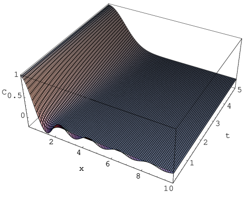
FIG. 2.: The ASD as a function of scaled frequency $x=\omega/\Delta$, and the parameter $t=1/g=L/\xi$.

To see this in more detail, let us consider approximations of Eq. (11) in various regimes of interest.

1. In the metallic regime $g>1$ for $x\ll g$ we obtain :

$$C(x)=\frac{\sin(\pi x)}{\pi x}\exp(-\frac{\pi^{3}}{6}\frac{1}{g}x^{2}),$$ (14)

where $x=\omega/\Delta$, which for $g\rightarrow\infty$ reduces to the result obtained with the unitary Wigner-Dyson ensemble of random matrices[12].

2. In the strongly localized regime $g\ll 1$, one obtains:

$$C(\omega)=\frac{\sin(gx)}{gx}\exp(-\frac{g}{2}\pi x^{2}).$$ (15)

Rescaling $\tilde{x}=(g/\pi)\omega/\Delta=(1/\pi)\omega/\Delta_{c}$, we note the similarity to Eq. (14).

This result shows clearly that the correlations between energy levels belonging to states which are spatially separated by more than the localization length $\xi$ are weak. As a result, the ASD shows only correlations with the period of twice the effective local energy level spacing $\pi~{}\Delta_{c}$ of energy levels whose wave functions overlap spatially.

As $g\rightarrow 0$, the function is dominated by the Gaussian factor. Thus, $C(\omega)=0$ exactly as $g\rightarrow 0$, and $\omega^{2}~{}>~{}\Delta^{2}/g$.

In Fig. 3 a plot of

$$F(t)=C(\Delta_{c})=\frac{\sin(\exp(-\pi t)-1)}{\exp(-\pi t)-1}$$ (16)

$$\exp(-\frac{1}{4}(-\exp(-2\pi t)+4\exp(-\pi t)-3+2\pi t)),$$ (17)

is shown, where $t=1/g=L/\xi$. The ASD is decaying from $1$ to $0$ as the frequency is held constant at $\omega=\Delta_{c}$ and one varies the length of the wire $L$ or the parameter $t$ in Fig. 3, compare with Fig. 1.

FIG. 3.: $F(t)$, as a function of the scaled length of the wire $t=1/g=L/\xi$.

IV Discussion

In summary, the ASD is established as a tool to study the level statistics of disordered metals. An analytical expression is obtained for the ASD of a quasi-1-dim. disordered mesoscopic wire. At frequencies below the mean level spacing $\Delta$ the ASD approaches 1 like a Gaussian for any value of the conductance g, and there is no information on localization in this regime. This was pointed out by Efetov [7] when studying the weakening of level repulsion by localization. It was stressed there, that the noncompact degrees of freedom are needed to describe localization that way. Here, it is shown that the information is rather contained in the large frequency correlations. The ASD shows a crossover to a strong damping of the correlations as the length of the wire exceeds the localization length $\xi$, accompanied by the convergence of the period of the strongly damped oscillations to the constant $2\pi\Delta_{c}$. Thus, the wire can be thought of as effectively separated into localization volumes, as obtained earlier in Refs. [18, 8].

One may argue that, since the averaging over the impurity potential was done before normalization, the resulting function might contain different information than the one obtained by normalizing for a given impurity potential before doing the averaging[19]. The goal of this article is however to show that level statistics can be characterized with the simplest tool, $C(\omega)$.

Now, it might become possible to address problems analytically, which could not be solved with the methods known so far, due to their complexity. While the ASD cannot contain any information on the eigenfunctions of the system, we have seen that it contains enough information to characterize the energy level statistics.

The function $F(t)$ may serve as a parameter characterizing localization : it is $1$ in the metallic regime and $0$, when all states at all energies are localized. It decays to approximately $1/e$ when the length of the wire coincides with the localization length, $L=\xi$.

In addition, recently it has been shown that the ASD can contain information not only on a metal-insulator-crossover, but also on a -transition, as demonstrated with the Anderson model on a Bethe lattice[15].

The author would like to thank Uzy Smilansky for drawing his attention to the ASD as a tool to study level statistics, and Thomas Dittrich, Konstantin Efetov, Dietrich Klakow, D. E. Khmel’nitskii, Igor Lerner, Daniel Miller, Vladimir Prigodin and Klaus Ziegler for usefull discussions, and Simon Villain- Guillot for critical reading of the manuscript.

This work was possible thanks to a scholarship by Minerva and support by the Max Planck Institute of Physics of Complex Systems in Dresden.

REFERENCES

- [1] present address, E- mail: ketteman@idefix.mpipks-dresden.mpg.de
- [2] P. W. Anderson, Phys. Rev. 109, 1492(1958).
- [3] N. F. Mott, W. D. Twose, Adv. Phys. 10, 107(1961).
- [4] D. J. Thouless, Phys. Rev. Lett. 39, 1167(1977).
- [5] P. W. Anderson, D. J. Thouless, E. Abrahams, D. S. Fisher Phys. Rev. B22, 3519 (1980); W. Weller, V. N. Prigodin, Y. A. Firsov, Phys. Stat. Sol. 110, 143(1982); N. Dorokhov, Sov. Phys. JETP Lett. 36, 318(1982); Sov. Phys. JETP 58, 606(1983).
- [6] K. B. Efetov, A. I. Larkin, Zh. Eksp Teor. Fiz. 85, 764(1983) ( Sov. Phys. JETP 58, 444 ).
- [7] K. B. Efetov, Adv. Phys. 32, 53 (1983); Supersymmetry in Disorder and Chaos (Cambridge University Press, Cambridge,1997).
- [8] A. Altland, D. Fuchs, Phys. Rev. Lett. 74, 4269(1995).
- [9] O. Agam, B. L. Altshuler and A. V. Andreev, Phys. Rev. Lett. 75, 4389 (1995).
- [10] A. Altland, Y. Gefen, G. Montambaux, Phys. Rev. Lett. 76, 1130(1996).
- [11] A. V. Andreev and B. D. Simmons, Phys. Rev. Lett. 75, 2304 (1995).
- [12] S. Kettemann, D. Klakow, U. Smilamsky, J. Phys. A,3643(1997).
- [13] F. Haake, M. Kus, H.- J. Sommers, H. Schomerus, and K. Zychowski, J. Phys. A 29, 3641(1996).
- [14] O. Bohigas, M. Giannoni, C. Schmit, Phys. Rev. Lett. 52, 1(1984).
- [15] S. Kettemann, unpublished(1998).
- [16] F. Wegner, Z. Phys. B 35, 207(1979); L. Schaefer, F. Wegner, Z. Phys. B 38, 113(1980).
- [17] K. B. Efetov, A. I. Larkin, D. E. Khmel’nitskii, Sov. Phys. JETP 52, 568(1980) ( Zh. Eksp. Teor. Fiz. 79, 1120(1980)).
- [18] S. Kettemann, K. B. Efetov, Phys. Rev. Lett. 74, 2547(1995).
- [19] K. Ziegler, I. Lerner, private discussion.