Logarithmic corrections of the avalanche distributions of sandpile models at the upper critical dimension

Abstract

We study numerically the dynamical properties of the BTW model on a square lattice for various dimensions. The aim of this investigation is to determine the value of the upper critical dimension where the avalanche distributions are characterized by the mean-field exponents. Our results are consistent with the assumption that the scaling behavior of the four-dimensional BTW model is characterized by the mean-field exponents with additional logarithmic corrections. We benefit in our analysis from the exact solution of the directed BTW model at the upper critical dimension which allows to derive how logarithmic corrections affect the scaling behavior at the upper critical dimension. Similar logarithmic corrections forms fit the numerical data for the four-dimensional BTW model, strongly suggesting that the value of the upper critical dimension is four.

]

I Introduction

The concept of self-organized criticality introduced by Bak, Tang, and Wiesenfeld allows to describe scale invariance in driven systems [2]. Sandpile models and especially the Bak-Tang-Wiesenfeld (BTW) sandpile model are known as the paradigm of self-organized criticality. The steady state dynamics of the system is characterized by the probability distributions for the occurrence of relaxation clusters of a certain size, area, duration, etc. Despite numerous theoretical efforts [3, 4, 5, 6] the values of the exponents of the probability distribution characterizing the critical behavior of the system were determined only numerically for $D=2$ and $D=3$ [7, 8]. These investigations are based on an accurate finite-size scaling analysis and were confirmed in a recently published work [9]. In higher dimensions the scaling behavior of the BTW model is still controversial. Especially, the value of the upper critical dimension $D_{u}$ where the mean-field solution describes the scaling behavior of the system is not known exactly. Whereas renormalization group approaches predicted $D_{u}=4$ [10, 11, 12] the results of numerical simulations are not consistent. Several authors were led by their investigations to the conjecture that $D_{u}=4$ [8, 13]. On the other hand comparable simulations in various dimension display no mean-field behavior for $D=4$ which was interpreted as an evidence that the values of the upper critical dimension is greater than four [9, 14].

In this paper we consider the BTW model in various dimensions and improve the accuracy of the analysis significantly. Our analysis reveals that the scaling behavior of the four dimensional model is characterized by the mean-field exponents with additional logarithmic corrections. We benefit in our analysis from the exact solution of the directed BTW model which displays logarithmic corrections at the upper critical dimension $D_{u}=3$ [15]. This solution is used in order to develop a scaling analysis for the directed BTW model which takes these logarithmic corrections into account. This type of scaling analysis will then be applied to the usual BTW model. The important result of this analysis is that the scaling behavior of the probability distributions as well as the usual finite-size scaling ansatz are affected by logarithmic corrections for $D=4$. These logarithmic corrections are a particular feature of the four-dimensional system and could not observed in higher dimensions. This suggest that the value of the upper critical dimension is indeed four.

II The BTW model

We consider the $D$-dimensional BTW model on a square lattice of linear size $L$ in which integer variables $E_{\bf r}\hskip 2.15277pt\raisebox{1.72218pt}{$\scriptstyle\geq$}\hskip 2.15277pt0$ represent local energies. One perturbes the system by adding particles at a randomly chosen site ${\bf r}$ according to

$$E_{\bf r}\,\mapsto\,E_{\bf r}+1\,.$$ (1)

A site is called unstable if the corresponding energy $E_{\bf r}$ exceeds a critical value $E_{c}$, i.e., if $E_{\bf r}\hskip 2.15277pt\raisebox{1.72218pt}{$\scriptstyle\geq$}\hskip 2.15277ptE_{c}$, where $E_{c}$ is given by $E_{c}=2D$. An unstable site relaxes, its energy is decreased by $E_{c}$ and the energy of the $2D$ next neighboring sites are increased by one unit, i.e.,

$$E_{\bf r}\;\to\;E_{\bf r}\,-\,E_{c}$$ (2)

$$E_{{\rm nn},\bf r}\;\to\;E_{{\rm nn},\bf r}\;+\;1.$$ (3)

In this way the neighboring sites may be activated and an avalanche of relaxation events may take place. The sites are updated in parallel until all sites are stable. Starting with a lattice of randomly distributed energies $E\in\{0,1,2,...,E_{c}-1\}$ the system is perturbed according to Eq. (1) and Dhar’s ’burning algorithm’ is applied in order to check if the system has reached the critical steady state [3]. Usually one studies several different quantities in order to characterize the avalanches: the number of relaxation events $s$ (size), the number of distinct toppled lattice site $a$ (area or volume), the duration $t$, and the radius $r$. In the critical steady state the corresponding probability distributions should obey power-law behavior characterized by exponents $\tau_{s}$, $\tau_{a}$, $\tau_{t}$ and $\tau_{r}$ according to

$$P_{x}(x)\,\sim\,x^{-{\tau_{x}}},$$ (4)

with $x\in\{s,a,t,r\}$. Because a particular lattice site may topple several times the number of toppling events exceeds the number of distinct toppled lattice sites, i.e., $s\hskip 2.15277pt\raisebox{1.72218pt}{$\scriptstyle\geq$}\hskip 2.15277pta$. It is known that multiple toppling events can be neglected for $D\hskip 2.15277pt\raisebox{1.72218pt}{$\scriptstyle\geq$}\hskip 2.15277pt3$ [8, 13], i.e., the distributions $P_{s}(s)$ and $P_{a}(a)$ display the same scaling behavior and especially $\tau_{s}=\tau_{a}$.

Scaling relations for the exponents $\tau_{s},\tau_{a},\tau_{t}$ and $\tau_{r}$ can be obtained if one assumes that the size, area, duration and radius scale as a power of each other, for instance

$$t\,\sim\,r^{\gamma_{tr}}.$$ (5)

The transformation law of probability distributions $P_{t}(t)\mbox{d}t=P_{r}(r)\mbox{d}r$ leads to the scaling relation

$${\gamma_{tr}}\;=\;\frac{\tau_{r}-1}{\tau_{t}-1}.$$ (6)

The scaling exponents $\gamma_{xx^{\prime}}$ are important for the description of the avalanches properties and their propagation. For instance the exponent $\gamma_{sa}$ indicates if multiple toppling events are relevant ($\gamma_{sa}>1$) or irrelevant ($\gamma_{sa}=1$). Since the exponent $\gamma_{ar}$ determine the scaling behavior of the avalanche area with its radius, $\gamma_{ar}$ is an appropriate tool to investigate whether the avalanche shape displays a fractal behavior or not. Finally, the exponent $\gamma_{tr}$ is usually identified with the dynamical exponent $z$.

The measurement of the probability distributions and the corresponding exponents [Eq. (4)] is affected by the finite system size $L$. If the avalanche exponents $\tau_{x}$ exhibit no system size dependence the finite-size scaling analysis could be applied [16]. In that case the probability distributions obey the scaling equation

$$P_{x}(x,L)\;=\;L^{-\beta_{x}}\,g_{x}(xL^{-\nu_{x}}),$$ (7)

where the exponents have to fulfill the scaling equation $\beta_{x}=\tau_{x}\nu_{x}$ [16]. The exponent $\nu_{x}$ determines the cut-off behavior of the probability distribution and it was shown that $\nu_{x}=\gamma_{xr}$ (see for instance [8]). The advantage of the finite size scaling analysis is that it yields additionally to the avalanche exponents $\tau_{x}$ the important scaling exponents: the avalanche dimension $\nu_{a}$, the dynamical exponent $\nu_{t}=z$, etc.

The value of the upper critical dimension $D_{u}$ of the undirected BTW model is not known rigorously. Several attempts were made to determine the value of $D_{u}$ using numerical simulations [8, 9, 13, 14]. Usually one considers the probability distributions and compares the avalanche exponents with the known mean-field values (see for instance [17]). But due to the limited computer power the implementation of the higher dimensional systems reduces considerably the system sizes $L$ and consequently also the straight portion of the probability distributions. This makes a determination of the avalanche exponents via regression very difficult for $D>3$. This disadvantage can be avoided by applying a finite-size scaling analysis. Our results obtained in this way are consistent with the assumption that $D_{u}=4$ and that the avalanche dimension is $v_{a}=4$ for $D\hskip 2.15277pt\raisebox{1.72218pt}{$\scriptstyle\geq$}\hskip 2.15277pt4$ [8].

Recently, Chessa et al. considered the BTW model in various dimensions using the same finite-size scaling analysis [9]. Compared to [8] they examined larger system sizes in $D\hskip 2.15277pt\raisebox{1.72218pt}{$\scriptstyle\geq$}\hskip 2.15277pt3$ and used an improved statistics (up to $10^{7}$ nonzero avalanches). From their results which differ for $D\hskip 2.15277pt\raisebox{1.72218pt}{$\scriptstyle\geq$}\hskip 2.15277pt4$ from those in [8] they concluded that $D=4$ is not the upper critical dimension. Especially they obtained from their finite-size scaling analysis $v_{a}\approx 3.5$ for the four-dimensional BTW model, i.e., the avalanches display a fractal behavior already for $D=4$. The origin of these conflicting results is that the used statistics ($2\times 10^{6}$ nonzero avalanches) in [8] is not sufficient. Especially the fluctuating data points at the cut-off of the distribution $P_{a}(a)$ lead to uncertain results (see Fig. 5 in [8]). For instance it is possible to obtain with this data a collapse of the distributions $P_{a}(a,L)$ for values of the avalanche dimension between $v_{a}=3.4$ and $v_{a}=4.1$.

Thus, there is no agreement in the literature on the behavior of the BTW model in different dimensions: Chessa et al. concluded from their analysis that the upper critical dimension is larger than four and that the avalanches displays fractility already for $D=4$. On the other hand there exist several theoretical approaches which leads to the conclusion that $D_{u}=4$: Real space [10] as well as momentum space [11, 12] renormalization group analysis predicted both $D_{u}=4$. From their exact solution of the BTW model on the Bethe lattice Majumdar and Dhar concluded that $D_{u}\hskip 2.15277pt\raisebox{1.72218pt}{$\scriptstyle\geq$}\hskip 2.15277pt4$ because the fractal dimension of avalanche clusters must be lower than that of the embedding space [18]. This leads the authors to the conjecture that the avalanches are compact for $D\hskip 2.15277pt\raisebox{1.72218pt}{$\scriptstyle\leq$}\hskip 2.15277ptD_{u}$ and fractal above the critical dimension. This fractility of the avalanche structure was already observed. Considering the avalanche propagation in higher dimension it was found that the avalanches are characterized by a compact activation front for $D=3$ and $D=4$. For $D>4$ the compact shape of the activation front is lost and several branches propagate through the system without coalesce together again (see Fig. 8 in [8]). Here, the avalanche propagation can be described as a branching process which is the main feature of the mean-field solution of sandpile models (see for instance [17]). Assuming that the clusters are compact and neglecting multiple toppling events (which is justified for $D=3$ and $D=4$ [8, 13]) Zhang derived in the continuum limit the equation $\tau_{a}=2-2/D$ [19] which gives the mean-field value $\tau_{a}=3/2$ again for $D=4$.

This incoherent picture of the behavior of the BTW model in higher dimensions leads us to reconsider the avalanche distributions again and compare our results with those of [9]. In contrast to our previous work [8] we use now larger system sizes ($L\hskip 2.15277pt\raisebox{1.72218pt}{$\scriptstyle\leq$}\hskip 2.15277pt128$ for $D=4$, $L\hskip 2.15277pt\raisebox{1.72218pt}{$\scriptstyle\leq$}\hskip 2.15277pt48$ for $D=5$, and $L\hskip 2.15277pt\raisebox{1.72218pt}{$\scriptstyle\leq$}\hskip 2.15277pt24$ for $D=6$) and increase the statistics significantly, i.e., we averaged all measurements over at least $5\times 10^{7}$ non-zero avalanches. As usual we measure the avalanche distributions [Eq. (4)] by counting the numbers of avalanches corresponding to a given area, duration, etc. and integrate these numbers over bins of increasing length (see for instance [20]). Successive bin length increases by a factor $b>1$. Throughout this work we performed all measurements with the factor $b=1.2$ since larger values of $b$ may change the cut-off shape of the distributions. Applying the finite-size scaling analysis this effect could lead to uncertain results for the scaling exponent $v_{a}$ (we found that this effect has to be taken into consideration at least for $b\hskip 2.15277pt\raisebox{1.72218pt}{$\scriptstyle\geq$}\hskip 2.15277pt1.5$).

FIG. 1.: The finite-size scaling exponents $\nu_{a}$ of the BTW model for various dimensions. The values of the exponents are obtained from the finite-size scaling analysis [Eq. (7)] of two probability distributions corresponding to two different system size $L_{1}$ and $L_{2}$ and are plotted as a function of $L=(L_{1}L_{2})^{1/2}$. In order to compare the different dimensions $\nu_{a}+1$ is plotted for $D=3$.

We focus our attention on the finite-size scaling analysis. Performing this analysis it is informative to produce the data-collapse not only for all curves corresponding to different system sizes but also to check the obtained data collapse for selected curves. For instance the finite-size scaling analysis of two curves corresponding to two successive system size ($L_{1}<L_{2}$) allows to check whether the actual scaling regime is already reached. This analysis is shown in Fig. 1 for the three-dimensional BTW model where it is known that finite-size scaling works for $L\hskip 2.15277pt\raisebox{1.72218pt}{$\scriptstyle\geq$}\hskip 2.15277pt64$ [8]. If one performs the finite-size scaling analysis for two system sizes with $L_{1}<L_{2}<64$ it is possible to obtain a data collapse (with small but systematic deviations, especially at the cut-off) but then the scaling exponents depend on the system sizes. In Fig. 1 we plot the scaling exponent $\nu_{a}(L_{1},L_{2})$ as a function of the average system size $L=(L_{1}L_{2})^{1/2}$. With increasing system sizes the exponent tends to the value $\nu_{a}=3$. For $L\hskip 2.15277pt\raisebox{1.72218pt}{$\scriptstyle\geq$}\hskip 2.15277pt64$ no significant system size dependence could be observed, i.e., a cross-over to the actual scaling regime where finite-size scaling works takes place at $L_{co}\approx 64$.

Analogous to the three-dimensional model we perform the same analysis for $D=4$, $D=5$, and $D=6$ and plot the obtained results in Fig. 1. It is remarkable that within the error-bars the values $\nu_{a}(D=3)+1$, $\nu_{a}(D=5)$, and $\nu_{a}(D=6)$ display for small system sizes the same finite-size dependence whereas the behavior of the four-dimensional system differs significantly from the other dimensions. The conjecture that the system size dependence of $\nu_{a}$ is independent of the dimension (except of the case $D=4$) implies that the cross-over to the actual scaling regime takes place at a comparable value $L_{co}\approx 64$. This could explain why the finite-size scaling analysis performed by Chessa et al. for $D\hskip 2.15277pt\raisebox{1.72218pt}{$\scriptstyle\geq$}\hskip 2.15277pt5$ yields exponents which are lower than the mean-field value $\nu_{a}=4$ [9]. Their considered system sizes for $D\hskip 2.15277pt\raisebox{1.72218pt}{$\scriptstyle\geq$}\hskip 2.15277pt5$ are outside the scaling regime where finite-size scaling works. Thus, they (and of course all other previous numerical investigations [8, 13, 14]) observed only the cross-over to the real scaling regime and not the real scaling behavior itself.

The significantly different behavior of the scaling exponent $\nu_{a}$ for $D=4$ (see Fig. 1) is remarkable since with increasing system size no cross-over to a scaling regime with a system size independent exponent $\nu_{a}$ could be observed. It seems that the scaling behavior of the four-dimensional model differs in principle from all other dimensions. A possible explanation is that the value of the upper critical dimension is $D_{u}=4$. Then the unique behavior of the exponent $\nu_{a}$ and the observed deviations to the expected pure mean-field scaling behavior for $D=4$ [9] could be explained by additional logarithmic corrections which affect the scaling behavior and which typically occur at the upper critical dimension.

In the rest of this paper we will show that our results are consistent with the assumption that the scaling behavior of the four-dimensional BTW model is characterized by the mean-field exponents with additional logarithmic corrections. In the next section we consider the BTW model with a preferred direction of the dynamics. This directed BTW model is exactly solved and it is known that logarithmic corrections occur for $D_{c}=3$ [15]. The directed BTW model is therefore a suitable paradigm to learn how the logarithmic corrections enters the scaling behavior at the upper critical dimension. This method of analysing will then be applied to the four dimensional BTW model in the last section.

III The directed BTW model at the upper critical dimension

In this section we consider the directed version of the BTW model which was introduced and exactly solved in all dimensions by Dhar and Ramaswamy [15]. Directed models are characterized by a preferred direction of the toppling rules. For instance a relaxation process takes place in a two-dimensional model if the energy of a given lattice site $(i,j)$ exceeds the critical value $E_{c}=D$:

$$E_{i,j}\; \to \;E_{i,j}\,-\,E_{c}$$ (8)

$$E_{i+1,j}\; \to \;E_{i+1,j}\,+\,E_{c}/D$$ (10)

$$E_{i,j+1}\; \to \;E_{i,j+1}\,+\,E_{c}/D.$$ (12)

One usually considers in simulations directed systems on a square lattice with periodic boundary conditions in the direction perpendicular to the preferred direction and open boundary conditions parallel to the preferred direction. The system is perturbed on the first line only (top of the pile) and particle could leave the system only on the last line (bottom of the pile).

Caused by the definition of the toppling rules no multiple toppling events can occur ($\Rightarrow\tau_{s}=\tau_{a}$). Since the perturbation takes place only on the top of the pile the average flux of particles through a surface in a given distance from the top is constant. This flux conservation leads to the scaling relation [15]

$$\tau_{a}\;=\;2-\frac{1}{\tau_{t}}.$$ (13)

According to Dhar and Ramaswamy the avalanche exponents of the two-dimensional model can be obtained by mapping the avalanche propagation onto a random walk and one gets $\tau_{a}=4/3$ and $\tau_{t}=3/2$, respectively.

For $D\hskip 2.15277pt\raisebox{1.72218pt}{$\scriptstyle\geq$}\hskip 2.15277pt3$ the exponents equal the mean-field values, i.e., $\tau_{a}=3/2$ and $\tau_{t}=2$, and additional logarithmic corrections to the power-law behavior occur in $D=3$ which is the value of the upper critical dimension [15]. A snapshot of several avalanches of the three-dimensional model are shown in Fig. 2. The shape of the avalanches reminds of a branching process which characterizes the avalanche propagation in the mean-field solution.

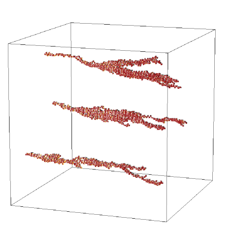
FIG. 2.: Snapshots of three arbritrary chosen avalanche of the directed BTW model at the upper critical dimension for $L=128$.

FIG. 3.: The probability distributions $P(t\hskip 2.15277pt\raisebox{1.72218pt}{$\scriptstyle\geq$}\hskip 2.15277ptT)$ of an avalanche of duration greater than or equal to $T$ for the directed BTW model at the upper critical dimension $D_{u}=3$. According to Eq. (15) $T\,P(t\hskip 2.15277pt\raisebox{1.72218pt}{$\scriptstyle\geq$}\hskip 2.15277ptT)$ is plotted as a function of $\ln{T}$. The dotted line is plotted to guide the eye.

According to the exact solution of Dhar and Ramaswamy the mean square flux $m(t)$ out of a given surface $t$ is given by

$$m(t)\;=\;\sum_{t^{\prime}=1}^{t}\,F(t^{\prime})$$ (14)

with $F(t)\sim 1/\ln{t}$ for $D=3$ [15]. Since the average flux through a surface $t$ is constant in the steady state the probability distribution of an avalanche of duration greater than or equal to $T$ scales in leading order as

$$P(t\hskip 2.15277pt\raisebox{1.72218pt}{$\scriptstyle\geq$}\hskip 2.15277ptT)\;\sim\;\frac{1}{m(T)}\;\sim\;\frac{\ln{T}}{T}.$$ (15)

The corresponding plot of the rescaled distribution $T\,P(t\hskip 2.15277pt\raisebox{1.72218pt}{$\scriptstyle\geq$}\hskip 2.15277ptT)$ as function of the duration in a logarithmic diagram is shown in Fig. 3 and confirms Eq. (15). The scaling behavior of the corresponding density distribution $P_{t}(t)$ is then given by

$$P_{t}(t)\;\sim\;\frac{\ln{t}}{t^{2}}.$$ (16)

In Fig. 4 we plot the rescaled distribution $P_{t}(t)/\ln{t}$ as a function of the duration $t$. The rescaled distribution exhibits a power-law behavior with the exponent $\tau_{t}=2$, in agreement with Eq. (16). The inset of Fig. 4 shows that a fit of the unscaled distribution $P_{t}(t)$ leads to lower values of the exponents $\tau_{t}$, i.e., a simple regression analysis can lead to the wrong result that the probability distributions are not characterized by the mean-field exponents.

The scaling behavior of the average avalanche duration $\langle t\rangle_{L}$ confirms the relevance of the logarithmic corrections. Using Eq. (16) the average duration is given by

$$\langle t\rangle_{L}\;=\;\int\limits^{t_{\rm max}}t\,P_{t}(t)\,\mbox{d}t\;\sim\;(\ln{L})^{2},$$ (17)

because in directed models the maximum value of the avalanche duration $t_{\rm max}$ equals the system size $L$. The scaling behavior of the average duration clearly displays the relevance of the logarithmic corrections since without these corrections the average duration scales as $\sim\ln{L}$. In order to confirm this result we plot in Fig. 5 the square root of the average duration as a function of the system size $L$ in a logarithmic diagram. The scaling behavior of the average duration agrees with Eq. (17).

FIG. 4.: The probability distributions $P_{t}(t)$ of the directed BTW model for $D=3$. According to Eq. (16) $P_{t}(t)/\ln{t}$ is plotted as a function of the duration $t$. The dashed line corresponds to a power-law with the exponent $\tau_{t}=2$. In the inset we plot $P_{t}(t)$ vs. $t$. Here, the curvature is caused by the logarithmic corrections. The inset shows that wrong results of the exponents were obtained if one does not take the logarithmic corrections into account.

FIG. 5.: The square root of the average avalanche distribution ${\langle t\rangle_{L}^{1/2}}$ vs. $L$ of the directed BTW model for $D=3$. The solid line corresponds to a logarithmic dependence of $\langle t\rangle_{L}^{1/2}$ according to Eq. (17).

The scaling behavior of the probability distribution $P_{a}(a)$ of the avalanche area displays also logarithmic corrections. The area $a$ of an avalanche of total duration $t$ is determined by the average number of toppling events in each surface $t^{\prime}\hskip 2.15277pt\raisebox{1.72218pt}{$\scriptstyle\leq$}\hskip 2.15277ptt$ (see [15]) and one gets to leading order

$$a(t)\;=\;\sum_{t^{\prime}=1}^{t}\,m(t)\;\sim\;\frac{t^{2}}{\ln{t}}.$$ (18)

Instead of the usual scaling behavior $a\sim t^{2}$ which is valid for $D>D_{u}$ the leading order of the area scales with the duration as $a\sim t^{2}/\ln{t}$. Since the maximum value of the duration $t_{\rm max}$ equals the system size the maximum avalanche area scales as

$$a_{\rm max}\;\sim\;\frac{L^{2}}{\ln{L}}.$$ (19)

The maximum area $a_{\rm max}$ determines the cut-off behavior of the probability distribution and Eq. (19) indicates that the usual finite-size scaling ansatz [Eq. (7)] has to be modified in the presence of logarithmic corrections. In the following we derive this modified finite-size scaling ansatz which describes the scaling behavior of the avalanche distribution $P_{a}(a)$ for $D=D_{u}$. We assume that the leading order of the probability distribution of the avalanche area is given by

$$P_{a}(a)\;\sim\;\frac{(\ln{a})^{x_{a}}}{a^{\tau_{a}}}$$ (20)

with the mean-field exponent $\tau_{a}=3/2$ and where the exponent of the logarithmic corrections $x_{a}$ has to be determined. Comparing Eq. (16) with Eq. (20) the corresponding exponent of the duration distribution is given by $x_{t}=1$. Using the transformation law for probability distributions $P_{a}(a){\rm d}a=P_{t}(t){\rm d}t$ one can derive the exponent $x_{a}$. Inserting Eq. (18) into Eq. (20) one gets

$$P_{a}[a(t)]\;\sim\;t^{-3}\,(\ln{t})^{x_{a}+3/2}\,\left(2-\frac{\ln{\ln{t}}}{\ln{t}}\right)^{x_{a}}$$ (21)

and analogous

$$\frac{{\rm d}a(t)}{{\rm d}t}\;\sim\;t\,\frac{2\ln{t}-1}{(\ln{t})^{2}}.$$ (22)

The term of leading order in the transformation law has to vanish and thus we get $x_{a}=1/2$.

Due to the logarithmic corrections of the probability distribution $P_{a}(a)$ the simple finite-size scaling ansatz Eq. (7) does not work. The simplest ansatz is to assume that the rescaled distribution $P_{a}(a)(\ln{a})^{x_{a}}$ obeys the finite-size scaling equation

$$P_{a}(a,L)\,(\ln{a})^{-x_{a}}\;\sim\;f(L)\;g(a/a_{\rm max})$$ (23)

with the universal function $g$ and where the scaling function $f(L)$ has to be determined. For low values of the argument of the universal function ($a\ll a_{\rm max}$) the rescaled probability distribution is independent of the system size and characterized by the power-law behavior $g(x)\sim x^{-\tau_{a}}$ only. Thus we obtain $f(L)\sim a_{\rm max}^{-\tau_{a}}$. Using the known scaling behavior of $a_{\rm max}$ we get the modified finite-scaling ansatz

$$P_{a}(a,L)\,(\ln{a})^{-x_{a}}\;=\;L^{-2\tau_{a}}\,(\ln{L})^{\tau_{a}}\,\;g(aL^{-2}\ln{L}).$$ (24)

We present the corresponding scaling plot in Fig. 6. The data collapse of the different curves corresponding to different system size $L$ confirms the above analysis.

FIG. 6.: The modified finite-size scaling plot of the probability distribution $P_{a}(a)$ of the directed BTW model for $D=3$. The data collapse of the different curves corresponding to different system sizes $L$ confirms Eq. (24). The dashed line corresponds to a power-law with the mean-field exponent $\tau_{a}=3/2$.

In summary we showed that the scaling behavior of the directed BTW model at the upper critical dimension is characterized by strong logarithmic corrections. These logarithmic corrections affect the usual probability distributions [Eq. (4)], the scaling equations [Eq. (5)], and the finite-size scaling analysis [Eq. (7)]. The corrections are relevant in the sense that one has to take them into account in order to describe the real scaling behavior, otherwise one gets wrong values for the exponents (see Fig. 4).

Additionally we simulated the directed BTW model for $D=4$ and performed a finite-size scaling analysis. In agreement with the exact solution of Dhar and Ramaswamy the simple finite-size scaling ansatz, i.e., without logarithmic corrections, works quite well and the corresponding exponents equal the mean-field exponents. Thus, the logarithmic corrections to the scaling behavior occur only at the upper critical dimension $D_{c}=3$ [15].

IV The undirected BTW model for $D=4$

In the following we return to the investigation of the undirected BTW model for $D=4$ and show that the avalanche distributions are characterized by logarithmic corrections comparable to the directed BTW model at the upper critical dimension. First we generalize the scaling equations by introducing certain exponents which describe the logarithmic corrections. Guided by our previous analysis we assume that the probability distributions are given by

$$P_{t}(t)\;\sim\;\frac{(\ln{t})^{x_{t}}}{t^{\tau_{t}}}\quad\mbox{\rm and}\quad P_{a}(a)\;\sim\;\frac{(\ln{a})^{x_{a}}}{a^{\tau_{a}}}.$$ (25)

The maximal avalanche duration and area which determine the cut-off behavior of the corresponding distributions should scale with the system size as

$$t_{\rm max}\;\sim\;\frac{L^{\nu_{t}}}{(\ln{L})^{N_{t}}}\quad\mbox{\rm and}\quad a_{\rm max}\;\sim\;\frac{L^{\nu_{a}}}{(\ln{L})^{N_{a}}}.$$ (26)

The fifth introduced exponent describes how the area scales with the duration

$$a(t)\;\sim\;\frac{t^{\gamma_{at}}}{(\ln{t})^{\Gamma_{at}}}.$$ (27)

At the upper critical dimension the avalanche and scaling exponents equal the mean-field values $\tau_{a}=3/2$, $\tau_{t}=2$, $\nu_{a}=4$, $\nu_{t}=2$, and $\gamma_{at}=2$. In this way the logarithmic corrections are determined by five non-negative exponents which have to fulfill two scaling relations. The transformation law of probability distributions leads to the first scaling equation:

$$P_{a}[a(t)]\,\frac{{\rm d}a(t)}{{\rm d}t}\,{\rm d}t\; = \;P_{t}(t)\,{\rm d}t$$ (28)

$$\Longrightarrow\quad\quad\quad\frac{\Gamma_{at}}{2}\; = \;x_{t}\,-\,x_{a},$$ (29)

where we make use of the equation $\gamma_{at}=(\tau_{t}-1)/(\tau_{a}-1)$ and assume that the term of leading order of the logarithmic corrections has to vanish. Under the condition that the scaling behavior of the leading order of the maximum avalanche area $a_{\rm max}$ is given by Eq. (26) and Eq. (27) we obtain the second scaling relation

$$a_{\rm max}\; = \;a(t_{\rm max})\;=\;\frac{L^{\nu_{t}\gamma_{at}}}{(\ln{L})^{N_{t}\gamma_{at}+\Gamma_{at}}}$$ (30)

$$\Longrightarrow\quad\quad\quad N_{a}\; = \;\Gamma_{at}\,+\,\gamma_{at}\,N_{t}.$$ (31)

Here, we use that the scaling exponents equal the avalanche dimension ($\nu_{a}=\gamma_{ar}$) and the dynamical exponent ($\nu_{t}=\gamma_{tr}$), respectively. The relation $\gamma_{tr}\gamma_{at}=\gamma_{ar}$ [14] leads to Eq. (31). Thus, the logarithmic corrections to the usual scaling behavior are determined by only three independent exponents.

Corresponding to the directed BTW model for $D=D_{u}$ we assume that the distributions obey the finite-size scaling ansatz

$$P_{t}(t,L)\,(\ln{t})^{-x_{t}}\;\sim\;f_{t}(L)\;g_{t}(t/t_{\rm max}),$$ (32)

$$P_{a}(a,L)\,(\ln{a})^{-x_{a}}\;\sim\;f_{a}(L)\;g_{a}(a/a_{\rm max}),$$ (33)

where the scaling functions $f_{t}$ and $f_{a}$ are given by

$$f_{t}(L)\;\sim\;L^{-\nu_{t}\tau_{t}}\;(\ln{L})^{N_{t}\tau_{t}},$$ (34)

$$f_{a}(L)\;\sim\;L^{-\nu_{a}\tau_{a}}\;(\ln{L})^{N_{a}\tau_{a}},$$ (35)

since for small values of the argument of the universal functions ($t\ll t_{\rm max}$ and $a\ll a_{\rm max}$) the probability distributions are independent of the system size. For $D=D_{u}$ the avalanche and scaling exponents equal the mean-field values $\tau_{a}=3/2$, $\tau_{t}=2$, $\nu_{a}=4$, and $\nu_{t}=2$. Thus the finite-size scaling analysis of the area and duration distribution gives the correction exponents $N_{t}$, $x_{t}$, $N_{a}$, $x_{a}$, and the obtained values have to fulfill the equation [Eq. (29) and Eq. (31)]

$$2(x_{t}-x_{a})\;=\;N_{a}\,-\,2N_{t}.$$ (36)

FIG. 7.: The system size dependence of the average avalanche duration ${\langle t\rangle_{L}}$ of the BTW model for $D=4$. To guide the eye we plot the solid line which corresponds to Eq. (37).

FIG. 8.: The modified finite-size scaling plot of the probability distribution $P_{t}(t)$ of the BTW model for $D=4$ and $L=24,32,40,48,56,64,72,80,96,128$. The data collapse of the different curves corresponding to different system sizes $L$ confirms Eq. (32). The dashed line corresponds to a power-law with the mean-field exponent $\tau_{t}=2$.

Analogous to the analysis of the directed BTW model we consider the scaling behavior of the average avalanche duration $\langle t\rangle_{L}$ before we apply the finite-size scaling analysis. According to Eq. (25) and Eq. (26) the average duration is given by

$$\langle t\rangle_{L}\;=\;\int\limits^{t_{\rm max}}t\,P_{t}(t)\,\mbox{d}t\;\sim\;\left(\ln{\frac{L^{2}}{(\ln{L})^{N_{t}}}}\right)^{x_{t}+1}$$ (37)

which allows additionally to the finite-size scaling analysis an independent determination of the exponents $x_{t}$ and $N_{t}$. We tried several values of $x_{t}$ and $N_{t}$ and obtained a good result for $x_{t}\approx 1/2$ and $N_{t}\approx 1/2$. In Fig. 7 we present in an logarithmic diagram $\langle t\rangle^{2/3}$ vs. $L^{2}/(\ln{L})^{1/2}$. The plotted values are located on a straight line, in agreement with Eq. (37).

These values are confirmed by the finite-size scaling analysis of the duration distribution $P_{t}(t)$ according to Eq. (32). A satisfying data collapse is obtained for $x_{t}=1/2$ and $N_{t}=1/2$ as one can see in Fig. 8.

FIG. 9.: The modified finite-size scaling plot of the probability distribution $P_{a}(a)$ of the BTW model for $D=4$ and $L=24,32,40,48,56,64,72,80,96,128$. The data collapse of the different curves corresponding to different system sizes $L$ confirms Eq. (33). The dashed line corresponds to a power-law with the mean-field exponent $\tau_{a}=3/2$.

Now we consider the finite-size scaling analysis of the area duration $P_{a}(a)$. Since the correction exponents have to fulfill Eq. (36) it must be possible to produce the data collapse of $P_{a}(a)$ by varying one parameter only if we assume that the above determined values $x_{t}=1/2$ and $N_{t}=1/2$ are correct. We eliminated $N_{a}$ in the scaling ansatz [Eq. (33) and Eq. (35)] and varied the exponent $x_{a}$. An almost perfect data collapse is obtained for $x_{a}\approx 1/4$. The corresponding scaling plot is shown in Fig. 9 and confirms the accuracy of the above determined exponents $x_{t}$ and $N_{t}$. In contrast to the three dimensional model, where the simple finite-size scaling works for $L\hskip 2.15277pt\raisebox{1.72218pt}{$\scriptstyle\geq$}\hskip 2.15277pt64$ [8], the finite-size behavior of the four-dimensional model are governed by the logarithmic corrections and the modified finite-size scaling ansatz works very well already for $L\hskip 2.15277pt\raisebox{1.72218pt}{$\scriptstyle\geq$}\hskip 2.15277pt24$. Finally we mention that Chessa et al. who used the simple finite-size scaling ansatz obtained a less accurate data collapse for $L\hskip 2.15277pt\raisebox{1.72218pt}{$\scriptstyle\geq$}\hskip 2.15277pt48$ [9] since they did not take the logarithmic corrections into account.

V Conclusions

We studied numerically the dynamical properties of the BTW model on a square lattice for $D\hskip 2.15277pt\raisebox{1.72218pt}{$\scriptstyle\geq$}\hskip 2.15277pt3$. Our investigation of the avalanche distribution which includes a careful examination of the finite-size corrections shows that analyses [8, 9] of the BTW model for $D\hskip 2.15277pt\raisebox{1.72218pt}{$\scriptstyle\geq$}\hskip 2.15277pt4$ are not conclusive. Our results are consistent with the assumption that the scaling behavior of the four-dimensional BTW model is characterized by the mean-field exponents with additional logarithmic corrections. We provide numerical tests for the theoretically predicted logarithmic correction terms for the directed BTW model at the upper critical dimension $D_{u}=3$. We introduce a refined finite-size scaling analysis which takes these logarithmic corrections into account. These logarithmic corrections occur for $D=4$ only, strongly suggesting that the value of the upper critical dimension is four. To proof this definitely in our opinion it is necessary to show that the distributions of the five dimensional model are characterized by the pure mean-field values. Unfortunately, due to the limited computer power it is at present impossible to consider the actual scaling regime for $D=5$.

- [1] E-mail: sven@thp.uni-duisburg.de
- [2] P. Bak, C. Tang and K. Wiesenfeld, Phys. Rev. Lett. 59, 381 (1987), Phys. Rev. A 38, 364 (1988).
- [3] D. Dhar, Phys. Rev. Lett. 64, 1613 (1990).
- [4] S. N. Majumdar and D. Dhar, J. Phys. A 24, L357 (1991). S. N. Majumdar and D. Dhar, Physica A 185, 129 (1992).
- [5] V. B. Priezzhev, J. Stat. Phys. 74, 955 (1994).
- [6] E. V. Ivashkevich, J. Phys. A 76, 3643 (1994).
- [7] S. Lübeck and K. D. Usadel, Phys. Rev. E 55, 4095 (1997).
- [8] S. Lübeck and K. D. Usadel, Phys. Rev. E 56, 5138 (1997).
- [9] A. Chessa, E. Marinari, A. Vespignani, and S. Zapperi, Phys. Rev. E 57, R6241 (1998).
- [10] S. P. Obukhov, in Random Fluctuations and Pattern Growth, edited by H. E. Stanley and N. Ostrowsky, Kluwer 1988 (Dordrecht, Netherlands).
- [11] A. Díaz-Guilera, Europhys. Lett. 26, 177 (1994).
- [12] A. Corral and A. Díaz-Guilera, Phys. Rev. E 55, 2434 (1997).
- [13] P. Grassberger and S. S. Manna, J. Phys. 51, 1077 (1990).
- [14] K. Christensen and Z. Olami, Phys. Rev. E 48, 3361 (1993).
- [15] D. Dhar and R. Ramaswamy, Phys. Rev. Lett. 63, 1659 (1989).
- [16] L. P. Kadanoff, S. R. Nagel, L. Wu and S. M. Zhou, Phys. Rev. A 39, 6524 (1989).
- [17] M. Vergeles, A. Maritan, and J. Banavar, Phys. Rev. E 55, 1998 (1997).
- [18] D. Dhar and S. N. Majumdar, J. Phys. A 23, 4333 (1990).
- [19] Y.-C. Zhang, Phys. Rev. Lett. 63, 470 (1989).
- [20] S. S. Manna, J. Phys. A 24, L363 (1991).