What do noise measurements reveal about fractional charge in FQH liquids?

Abstract

We present a calculation of noise in the tunneling current through junctions between two two-dimensional electron gases (2DEG) in inequivalent Laughlin fractional quantum Hall (FQH) states, as a function of voltage and temperature. We discuss the interpretation of measurements of suppressed shot noise levels of tunneling currents through a quantum point contact (QPC) in terms of tunneling of fractionally charged states. We show that although this interpretation is always possible, for junctions between different FQH states the fractionally charged states involved in the tunneling process are not the Laughlin quasiparticles of the isolated FQH states that make up the junction, and should be regarded instead as solitons of the coupled system. The charge of the soliton is, in units of the electron charge, the harmonic average of the filling fractions of the individual Laughlin states, which also coincides with the saturation value of the differential conductance of the QPC. For the especially interesting case of a QPC between states at filling fractions $\nu=1$ and $\nu={\frac{1}{3}}$, we calculate the noise in the tunneling current exactly for all voltages and temperatures and investigate the crossovers. These results can be tested by noise experiments on $(1,{\frac{1}{3}})$ QPCs. We present a generalization of these results for QPC’s of arbitrary Laughlin fractions in their weak and strong coupling regimes. We also introduce generalized Wilson ratios for the noise in the shot and thermal limits. These ratios are universal scaling functions of $V/T$ that can be measured experimentally in a general QPC geometry.

I INTRODUCTION

Recently, two experimental groups, in Saclay [1] and at the Weizmann Institute [2], have been able to measure suppressed shot noise in a quantum point contact (QPC) geometry - a constriction in the plane of a 2DEG. In this setup the two edges of the FQH system are brought together by applying a gate voltage that creates the QPC. In what follows we will refer to this particular geometry as tunneling between the edges of the same FQH system (see Fig. 1(a)). The quantum shot noise in this case reflects the fluctuations in the tunneling current that result from the presence of the constriction. The results obtained in these experiments for FQH systems at filling fraction $\nu=1/3$ are consistent with the interpretation of uncorrelated tunneling events of fractionally charged quasiparticles ($e^{*}=e/3$) between the edges of the FQH system at the QPC.

At filling fraction $\nu={\frac{1}{3}}$, the Hall conductance and the fractional charge of the quasiparticles are determined by the same universal coefficient, the filling fraction. Thus, it is natural to ask if the noise experiments measure the fractional charge or the conductance. Clearly, one way to address this issue is to extend these measurements to a range of filling fractions not in the Laughlin sequence, where the charges of the quasiparticles (in units of $e$) are not equal to the filling fraction. However, the theory of tunneling in generic FQH states is only understood qualitatively and many important issues, such as edge reconstructions, still need to be understood. In contrast, there exists a rather detailed and well understood theory of tunneling between the edges of the Laughlin states.

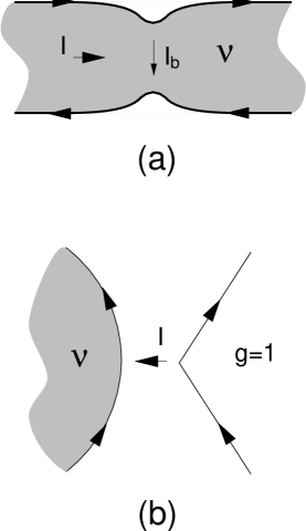
FIG. 1.: Different geometries for measuring shot noise in FQH systems: a) Geometry with tunneling between the edges of the same FQH systems with filling fraction $\nu$; b) Geometry with tunneling between the edges of two different FQH system with filling fractions $\nu$ and 1 (representing a normal metal) respectively.

Shot noise measurements can be an important probe of the edges of FQH states in other, more general, geometries. From this point of view, we consider the problem of tunneling from a Fermi liquid (i. e., $\nu=1$) to a Laughlin FQH state at filling fraction $\nu$ or, more generally, between FQH edge states with different filling fractions, $(\nu_{1},\nu_{2})$. An instructive example is presented in Fig. 1(b) which is a schematic representation inspired by the geometry used in the experiments by A. Chang and coworkers [3, 4].

A possible experimental realization of the geometry depicted in Fig. 1 (b) is suggested in Fig. 2, where the strong tunneling region or “hot spot” is assumed to be designed to be small, of the order of a few cyclotron lengths. These sizes are similar to the ones in the QPC experiments of Refs. [1, 2].

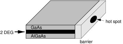
FIG. 2.: A possible experimental realization of the QPC junction between an electron gas and a FQH liquid, inspired by the cleaved edge overgrowth samples of A. Chang and coworkers. The electron gas reservoirs make contact to the FQH liquid formed in the 2DEG via tunneling through a “hot spot”, where the barrier is made weaker. This tunneling region should be small, of the order of a few cyclotron lengths.

In this paper we consider the more general problem of non-equilibrium noise in tunnel junctions between different FQH states. We will show here that, while noise measurements always constitute a detailed probe of the theory of the edge states, their interpretation in terms of the (generally fractional) charges of the quasiparticles is actually quite subtle. In particular, it is both natural and important to inquire if measurements of suppressed shot noise level in a generic QPC junction provide unambiguous evidence for fractional charge in the isolated FQH fluid and what is its relation with the conductance. In the example that we will discuss here, we will find that the level of the shot noise in the weak backscattering regime tracks the differential conductance of the junction instead of being determined by the (fractional) charge of the FQH quasiparticles or by the electron charge. In fact, we will also discuss an example in which in a two-terminal measurement of the shot noise level, it is impossible to distinguish between tunneling of electrons between the edges of identical Laughlin states and electrons between (carefully chosen) different FQH states (see Fig. 3), for instance $({\frac{1}{3}},{\frac{1}{3}})$ and $({\frac{1}{5}},1)$. Logically, there are two related issues involved in this problem. One is the charge of the quasiparticle participating in the tunneling process, and another are the properties of the isolated fluids connected by the junction.

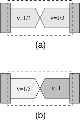
FIG. 3.: Two different junctions $(\nu_{1},\nu_{2})$ which cannot be told apart if one only looks at the two-terminal properties measured outside of the dashed region. The effective Luttinger parameter $g=\frac{2\nu_{1}\nu_{2}}{\nu_{1}+\nu_{2}}$ is the same in both cases. Therefore, the $(\frac{1}{3},\frac{1}{3})$ junction in (a) and the $(\frac{1}{5},1)$ junction in (b) have both: i) the same asymptotic conductance at large voltages $G=\frac{1}{3}\frac{e^{2}}{h}$, ii) the same shot noise level $S=2eI$ for small voltages, and iii) the same shot noise level $S=2\frac{e}{3}I_{b}$ for small backscattering currents $I_{b}=GV-I$

Let us begin by reviewing the basic theoretical assumptions and interpretations involved in the various studies of noise in tunneling between Luttinger liquids [5, 6, 7, 8, 9, 10]. Within the theoretical framework of tunneling between the edges of a given FQH system, the low temperature (shot) noise spectrum $S$ is calculated in terms of the correlation function of the tunneling current, which in the geometry of Fig. 1 (a) corresponds to the backscattering current $I_{b}$. In this limit, the shot noise level $S$ is

$$S=2qI_{b}$$ (1)

This result can be interpreted as meaning that the backscattering current is due to ‘uncorrelated’ tunneling of Laughlin quasiparticles carrying fractional charge, i.e., the current corresponds to a sequence of uncorrelated Poisson distributed quasiparticles that tunnel through the QPC. This result applies provided the backscattering current $I_{b}$ is arbitrarily small. Thus, the shot noise level for small tunneling currents reflects the charge of the carriers and, consequently, in the geometry of Fig. 1 (a), it measures the fractional charge. Alternatively, in the same geometry, we may also regard the transmission current as being carried by electrons, which are strongly correlated. This description corresponds to the dual picture of Ref. [11]. In this picture, defects in the transmission of electrons correspond to backscattering of kinks (i. e., “magnetic charges”) or quasiparticles. Thus, in this representation, the suppression factor in the shot noise level is a measure of the correlations among the electrons. In this dual picture, although the transmission current is large, the fluctuations of this current (i. e., the noise) are small and due to defects (or kinks) which play the role of the backscattering current $I_{b}$ in the quasiparticle picture.

Naturally, both pictures are completely equivalent and consistent with each other, and they yield the same result, as they should. Nevertheless, it is worth to stress that the physical interpretation of the coefficient $q$ of the shot noise as the charge of the quasiparticle of the FQH state is not based on a direct measurement of the charge. Instead, this interpretation relies on the existence of the quasiparticle picture since it is precisely the tunneling of quasiparticles which causes the fluctuations of the current in that picture. This interpretation is physically consistent because it is possible to determine independently by a transport measurement that the 2DEG is in a Laughlin state.

From a conceptual point of view it is then natural to ask if it is always possible to find an analog of the quasiparticle picture in which the coefficient of the shot noise is always necessarily determined by the charge of a physical eigenstate of an isolated FQH state. We will see now that answering this question leads to an interesting paradox, shown in Fig. 3. Let us reexamine the problem of quasiparticle tunneling between the edges of a $\nu={\frac{1}{3}}$ Laughlin state but as seen from the dual picture. In this representation, we have electrons tunneling between two $\nu={\frac{1}{3}}$ Laughlin states. It turns out that, using the methods of ref. [12], it is straightforward to show (see below) that this tunnel junction is equivalent to a tunnel junction between Laughlin states $\nu=1$ and $\nu={\frac{1}{5}}$ in which electrons hop between the two fluids at the QPC. The paradox resides in the fact that the noise in the tunneling current is determined by a coefficient which is still $q={\frac{1}{3}}$ in spite of the fact that there are no such quasiparticles in the bulk of the isolated $\nu=1$ and $\nu={\frac{1}{5}}$ states. In this picture, $q={\frac{1}{3}}$ is the charge of the soliton which diagonalizes the junction Hamiltonian. From the point of view of a $(1,{\frac{1}{5}})$ junction, these states are complicated non-local superpositions of the quantum states of the two isolated inequivalent FQH fluids. The only way to distinguish cases (a) and (b) in Fig. 3 is to determine the conductance of the fluids independently through a four-terminal measurement. In fact, a two-terminal measurement cannot distinguish these two cases. It is also worth to remark that, as we will see below, the coefficient of the noise level of picture (b) in Fig. 3, is precisely the same (in units of ${\frac{e^{2}}{h}}$) as the saturation value of the differential conductance of the $(1,{\frac{1}{5}})$ junction!

One may also ask, given a QPC between two inequivalent FQH states, if it is always possible to find an equivalent system in which the noise in the tunneling current can be interpreted as due to tunneling of quasiparticles of isolated FQH fluids. The answer to this question is no. We will see below that a generic QPC $(\nu_{1},\nu_{2})$, for the Laughlin states $\nu_{i}^{-1}=2k_{i}+1$ and $k_{i}\in{\bf Z}$ ($i=1,2$), is equivalent to the QPC $(\nu_{eff},\nu_{eff})$ with $\nu_{eff}^{-1}=k_{1}+k_{2}+1$. Hence, the equivalent junction represents tunneling between fermion Laughlin states only if either $k_{1}$ or $k_{2}$ (but not both) are odd integers. However, what it is always true, is the statement that the noise level is determined by the charge of the soliton (kinks) states that diagonalize the Hamiltonian of the junction and, in general, these states cannot be represented simply in terms of the quasiparticles of the isolated fluids. Superficially, this result may appear to violate the basic bulk-edge correspondence which is crucial for the theory of edge states of FQH fluids[13], as it involves tunneling of objects which are neither electrons nor quasiparticles of the isolated fluids. Actually, as we discuss below (see also the appendix of Ref. [14]), this is not a real paradox or contradiction since the edges are gapless and the structure of the Hilbert space is respected by these tunneling processes.

Measurements of noise, in addition to being useful tools to investigate experimentally the problem of fractional charge in FQH fluids, can also be used to probe the properties of the edges in greater detail. For instance, for the special and exactly solvable case of the $(1,{\frac{1}{3}})$ junction, we calculate the current correlation functions exactly for all voltages, temperatures and tunneling amplitudes, and show that the temperature and voltage dependence of the noise contains a great deal of information on the edge states, on the fixed points of the junctions and of their crossovers. For a generic $(\nu_{1},\nu_{2})$ junction, for which the correlation functions cannot be computed exactly, we find the noise in the asymptotic regimes of large and small voltages, and for high and low temperatures. The results are discussed in the form of a phase (or rather, crossover) diagram. To analyze the information obtained from the asymptotic regimes, we introduce a generalization of Wilson ratios useful in quantum impurity problems [16]. We define a generalized Wilson ratio as the quotient between the shot noise and the thermal noise levels. Near the two fixed points this ratio becomes a universal scaling function of $V/T$ independent of the coupling constant. The ratio contains information on the Luttinger liquid behavior through the parameter $g^{\prime}$ both in the exponent of the $V/T$ dependence and in the constant $g^{\prime}$ dependent prefactor. The ratios in the two fixed points are also related by duality. Finally, these ratios can be used to analyze the experimental data from both limits of thermal and shot noise in a unified way.

The paper is organized as follows. In Section II we review the model of Refs. [12, 14] and we introduce the relations among the charge densities of the rotated and the dual fields. We also define the backscattering current $I_{b}$ and introduce the definitions for the noise in both currents $S_{I}$ and $S_{I_{b}}$. In section III we discuss a generic junction between two FQH states at filling fractions $\nu_{1}$ and $\nu_{2}$. Here we give a general result for the current shot noise at both small and large tunneling amplitudes. In Section IV we consider in detail the $(1,{\frac{1}{3}})$ junction. Here we review (briefly) the refermionization procedure used to diagonalize exactly the Hamiltonian for this junction [10]. For this particular case, we calculate the noise at zero temperature in the current through the junction. We show that the noise in the limit of strong coupling (or weak backscattering current) is not a direct measurement of the fractional charge of the decoupled FQH fluid but, instead, it measures the charge of the soliton that diagonalizes the Hamiltonian, which also determines the saturation value of the conductance of the junction. In Section V we calculate the noise in the current $I$ and the backscattering current $I_{b}$ as a function of temperature $T$ and voltage $V$. We present our results in the form of a $T-V$ diagram for the noise. In particular, we show that the strong coupling regime relates the equilibrium and non-equilibrium regimes of the junction. The weak coupling region characterizes the regime of low temperatures and low voltages. We introduce ratios between the thermal and shot noise limits for both currents $I$ and $I_{b}$. In section VI we define generalized Wilson ratios as quotients between noise in the thermal and shot noise regimes for junctions with a generic value of $g^{\prime}$ using perturbative methods. These ratios are universal scaling functions of $V/T$ around both the weak and the strong coupling fixed points. In particular, we calculate the value of these ratios for the geometry depicted in Fig. 1 (a) used in recent experiments by L. Saminadayar et. al[1] and R. de Picciotto[2] for a $(\frac{1}{3},\frac{1}{3})$ junction. In section VII we discuss a four probe geometry and calculate the noise in all four channels. We show that, as a consequence of chirality, the noise in the incoming channels is insensitive to the presence of the QPC; it is given by the Johnson-Nyquist noise level, and it is proportional to the conductance determined by the respective filling fraction in either side of the junction. The noise in the outgoing channels, on the other hand, contains the information on the tunneling coupling, and depends on both filling fractions $\nu_{1}$ and $\nu_{2}$. Finally, in SectionVIII we summarize our main results and discuss its experimental implications.

II Model for the junction

In this section we review the model for a mismatched FQH junction used in Ref.[14]. We start with a Lagrangian for the FQH-normal metal junction that describes the dynamics on the edge of a FQH liquid, the electron gas reservoirs, and the tunneling between them through a single point-contact of the form

$${\cal L}={\cal L}_{edge}+{\cal L}_{res}+{\cal L}_{tun}\,.$$ (2)

The dynamics of the edge of the FQH liquid with a Laughlin filling fraction $\nu=\frac{1}{2k+1}$ is described by a free chiral boson field $\phi_{1}$ with the Lagrangian [15]

$${\cal L}_{edge}=\frac{1}{4\pi}\partial_{x}\phi_{1}(\partial_{t}-\partial_{x})\phi_{1}\,.$$ (3)

The edge electron and quasiparticle operators are given by

$$\psi_{e}\propto\,:e^{-i\frac{1}{\sqrt{\nu}}\phi_{1}(x,t)}:\,\,\,;\,\,\,\psi_{qp}\propto\,:e^{-i\sqrt{\nu}\phi_{1}(x,t)}:$$ (4)

${\cal L}_{res}$ describes the dynamics of the electron gas reservoir. As shown in Ref. [12], a 2D or 3D electron gas can be mapped to a 1D chiral Fermi liquid (FL) ($\nu=1$) when the tunneling is through a single point-contact. This 1D chiral Fermi liquid is represented by a free chiral boson field $\phi_{2}$. ${\cal L}_{res}$ is given by

$${\cal L}_{res}=\frac{1}{4\pi}\partial_{x}\phi_{2}(\partial_{t}-\partial_{x})\phi_{2}\,.$$ (5)

In this case, the electron operator is given by

$$\psi_{res}\propto:e^{-i\phi_{2}(x,t)}:$$ (6)

The tunneling Lagrangian between the FQH system and the reservoir is

$${\cal L}_{tun}=\Gamma\;\delta(x)\;e^{-i\omega_{0}t}\;:e^{i[\frac{1}{\sqrt{\nu}}\phi_{1}(x,t)-\phi_{2}(x,t)]}:+{\rm h.\ c.\ }\,,$$ (7)

where $\Gamma$ represents the strength of the electron tunneling amplitude which takes place at a single point in space $x=0$, the QPC. In what follows, by analogy with quantum impurity problems, we will refer to the QPC as the impurity.

The voltage difference between the two sides of the junction is introduced in the model by letting $\Gamma\rightarrow\Gamma e^{-i\omega_{0}t}$, where $\omega_{0}=eV/\hbar$. The external voltage $V$ can be interpreted as the difference between the chemical potentials of the two systems: $V=\mu_{1}-\mu_{\nu}$.

The density operators at both sides of the junction are defined as follows:

$$\rho_{1}=\frac{\sqrt{\nu}}{2\pi}\partial_{x}\phi_{1}\,\;,\;\;\;\;\;\rho_{2}=\frac{1}{2\pi}\partial_{x}\phi_{2}$$ (8)

By a suitable rotation the original Lagrangian ${\cal L}$ can be mapped into a new one [12, 14]:

$${\cal L} = \frac{1}{4\pi}\partial_{x}\phi^{\prime}_{1}(\partial_{t}-\partial_{x})\phi^{\prime}_{1}+\frac{1}{4\pi}\partial_{x}\phi^{\prime}_{2}(\partial_{t}-\partial_{x})\phi^{\prime}_{2}$$ (9)

$$\ +\Gamma\,\delta(x)\,e^{-i\omega_{0}t}e^{i\frac{1}{\sqrt{g^{\prime}}}[\phi^{\prime}_{1}(x,t)-\phi^{\prime}_{2}(x,t)]}+h.c.$$ (10)

where the new fields $\phi^{\prime}_{1}$ and $\phi^{\prime}_{2}$ have been introduced, and $g^{\prime}$ is an effective Luttinger parameter (which can also be regarded as an “effective filling fraction”) given by:

$$g^{\prime-1}=\frac{(1+\nu^{-1})}{2}.$$ (11)

In particular, this rotation relates the densities as follows:

$$\left(\matrix{\rho_{1}\cr\rho_{2}}\right)=\left(\matrix{\frac{1+\sqrt{\nu}}{2}&\frac{\sqrt{\nu}-1}{2}\cr\frac{1-\sqrt{\nu}}{2\sqrt{\nu}}&\frac{1+\sqrt{\nu}}{2\sqrt{\nu}}}\right)\left(\matrix{\rho^{\prime}_{1}\cr\rho^{\prime}_{2}}\right)$$ (12)

Next, we introduce the fields $\phi_{-}$ and $\phi_{+}$ that separate ${\cal L}$ into two decoupled Lagrangians ${\cal L}_{+}$ and ${\cal L}_{-}$,

$$\phi_{+}=\frac{\phi^{\prime}_{1}+\phi^{\prime}_{2}}{\sqrt{2}}\,\;,\;\phi_{-}=\frac{\phi^{\prime}_{1}-\phi^{\prime}_{2}}{\sqrt{2}}.$$ (13)

The densities associated with these new fields are defined as

$$\rho_{\pm}=\frac{1}{2\pi}\partial_{x}\phi_{\pm}$$ (14)

and they are related to the densities of the $\varphi^{\prime}_{1}$ and $\varphi^{\prime}_{2}$ fields by

$$\left(\matrix{\rho^{\prime}_{1}\cr\rho^{\prime}_{2}}\right)=\sqrt{\frac{g^{\prime}}{2}}\left(\matrix{1&1\cr 1&-1}\right)\left(\matrix{\rho_{+}\cr\rho_{-}}\right)$$ (15)

The successive rotations are schematized in Fig.(4).

FIG. 4.: Set of rotations from $\phi_{1,2}$ to $\phi_{\pm}$. The first rotation maps the original junction between two different FQH liquids to one between FQH with the same filling fraction $g^{\prime}$, the second one decouples the problem into two separate ones.

In terms of the $\phi_{\pm}$ fields the total Lagrangian reads:

$${\cal L} = \frac{1}{4\pi}\partial_{x}\phi_{+}(\partial_{t}-\partial_{x})\phi_{+}+\frac{1}{4\pi}\partial_{x}\phi_{-}(\partial_{t}-\partial_{x})\phi_{-}$$ (16)

$$+ \Gamma\delta(x)e^{-i\omega_{0}t}e^{\sqrt{\frac{2}{g^{\prime}}}\phi_{-}(x,t)}+h.c.$$ (17)

The strong coupling limit of this system is considerably simpler in the dual picture described by the dual fields ${\tilde{\phi}}_{\pm}$. In terms of the dual fields the effective Lagrangian has a new Luttinger parameter ${\tilde{g}}^{\prime}=1/g^{\prime}$ and an effective tunneling amplitude ${\tilde{\Gamma}}\sim\Gamma^{-{\frac{1+\nu}{2\nu}}}$. The (dual) Lagrangian is

$${\tilde{\cal L}} = \frac{1}{4\pi}\partial_{x}{\tilde{\phi}}_{+}(\partial_{t}-\partial_{x}){\tilde{\phi}}_{+}+\frac{1}{4\pi}\partial_{x}{\tilde{\phi}}_{-}(\partial_{t}-\partial_{x}){\tilde{\phi}}_{-}$$ (18)

$$+ {\tilde{\Gamma}}\delta(x)e^{-i\omega_{0}t}e^{\sqrt{2g^{\prime}}{\tilde{\phi}}_{-}(x,t)}+h.c.$$ (19)

The dual transformation in the strong coupling limit ($\Gamma\rightarrow\infty$ or ${\tilde{\Gamma}}=0$) can be expressed in terms of the fields $\phi^{\prime}_{1}$ and $\phi^{\prime}_{2}$:

$$\phi^{\prime}_{1} = \tilde{\phi}^{\prime}_{1}\Theta(-x)+\tilde{\phi}^{\prime}_{2}\Theta(x)$$ (20)

$$\phi^{\prime}_{2} = \tilde{\phi}^{\prime}_{2}\Theta(-x)+\tilde{\phi}^{\prime}_{1}\Theta(x)\ .$$ (21)

(here $\Theta(x)$ is the step function). The expectation values that appear in the correlation functions are taken with respect to the dual Lagrangian (with effective Luttinger parameter 1/g’ and coupling constant ${\tilde{\Gamma}}$). As mentioned above, the duality transformation relates the densities of the original fields and the densities of the dual fields. Notice that the densities in the incoming channels of the original fields $\rho^{\prime}_{1,2}(x<0)$, are the same as the densities in the incoming channels of the dual fields ${\tilde{\rho}}_{1,2}(x<0)$, i.e. the matrices given by Eqs. (12, 13) can be used to express the original fields $\phi_{1,2}(x<0)$ in terms of the fields ${\tilde{\phi}}_{+,-}(x<0)$. In order to write the densities in the outgoing channels of the original fields $\rho_{1,2}(x>0)$ in terms of the fields ${\tilde{\phi}}_{+,-}(x>0)$ it is necessary to realize that the duality transformation exchanges $\phi^{\prime}_{1}$ and $\phi^{\prime}_{2}$ for $x>0$. As a consequence, for $x>0$ Eq.(12) reads:

$$\left(\matrix{\rho_{1}\cr\rho_{2}}\right)=\left(\matrix{\frac{1+\sqrt{\nu}}{2}&\frac{\sqrt{\nu}-1}{2}\cr\frac{1-\sqrt{\nu}}{2\sqrt{\nu}}&\frac{1+\sqrt{\nu}}{2\sqrt{\nu}}}\right)\left(\matrix{\tilde{\rho}^{\prime}_{2}\cr\tilde{\rho}^{\prime}_{1}}\right)$$ (22)

Let us now use this formulation of the junction to calculate the current correlation functions, necessary to compute both the current through the junction and the noise. As shown in Fig. (5) there are incoming ($x<0$) and outgoing ($x>0$) scattering states with respect to the impurity location ($x=0$).

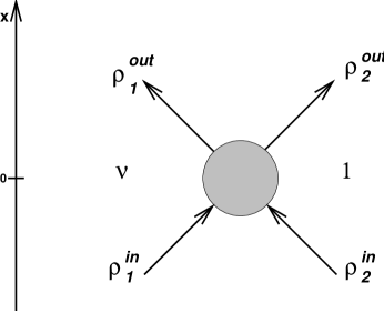
FIG. 5.: Four probe geometry for measurement of noise. The incident currents are those at $x<0$ while the outgoing currents are at $x>0$.

The current flowing from the reservoir (or $\nu=1$ state) to the filling fraction $\nu$ FQH state, can be written in terms of the imbalance of the densities before ($x=0_{-}$) and after the impurity ($x=0_{+})$:

$$I=\rho_{1}^{\rm out}-\rho_{1}^{\rm in}=\rho_{2}^{\rm in}-\rho_{2}^{\rm out}\ \$$ (23)

Likewise, the current $I^{\prime}$ and the densities $\rho^{\prime}$ of the rotated fields are related by

$$I^{\prime}=\rho^{\prime\rm out}_{1}-\rho^{\prime\rm in}_{1}=\rho^{\prime\rm in}_{2}-\rho^{\prime\rm out}_{2}\ \$$ (24)

As a consequence of current conservation and crossing symmetry (see Fig. 5) it follows that

$$I=I^{\prime}$$ (25)

Notice that Eqs. (23-25) are operator identities and not just relations between quantum averages.

The quantum noise for the current $I$, $S_{I}(\omega)$, is defined to be

$$S_{I}(\omega)\equiv\int_{-\infty}^{\infty}dt\;\cos\omega t\;\langle\{I(t),I(0)\}\rangle\ \$$ (26)

The noise $S_{I}(\omega)$ defined in Eq. (26) is, in general, a function of the tunneling amplitude $\Gamma$, the voltage $V$ and the temperature $T$. For the purpose of clarifying the physics, we will separate the contributions to the noise into an equilibrium piece, $S_{I}^{\rm eq}$, and an excess piece, $S_{I}^{\rm ex}$. The latter, as the name suggests, is the amount by which the noise, in the presence of a voltage $V$, exceeds the equilibrium ($V=0$) level.

Along the same lines, we can study the noise in the backscattering current. The backscattering current $I_{b}$ is defined by (see Fig. 6):

$$I_{b}=I_{m}-I$$ (27)

where the current $I_{m}$ is the limiting value of $I$ in the strong coupling (or large voltage) regime,i. e., the maximum current through the junction. Because of the operator identity between $I$ and $I^{\prime}$ (the current in the rotated system), $I_{m}=I^{\prime}_{m}$. $I_{m}$ has the following properties [5, 6, 7, 8, 9, 10, 11, 12]: its mean value is $\langle I_{m}\rangle=g^{\prime}\;{\frac{e^{2}}{h}}\;V$ and it is a dissipationless current ,i. e., its noise spectrum is completely determined by the value of the conductance:

$$S_{I_{m}}(\omega)=g^{\prime}{\frac{e^{2}}{2\pi}}|\omega|\coth{\frac{|\omega|}{2T}}\ \ .$$ (28)

From the definition of $I_{b}$ and the identity $I_{m}=I^{\prime}_{m}$, it follows that $I_{b}=I^{\prime}_{b}$. Its noise is defined naturally as

$$S_{I_{b}}(\omega)\equiv\int_{-\infty}^{\infty}dt\;\cos\omega t\;\langle\{I_{b}(t),I_{b}(0)\}\rangle\ \$$ (29)

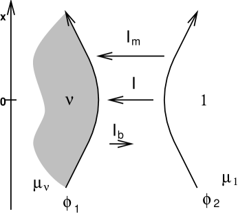
FIG. 6.: Backscattering current $I_{b}$. $I$ is the current through the junction for $\Gamma\neq 0$ and $I_{m}$ is the maximum current through the junction.

III Shot noise for a mismatched junction

The procedure outlined in the previous section can be generalized for a junction between two FQH liquids with filling fractions $\nu_{1},\nu_{2}$. In this case the effective filling fraction $g^{\prime}$ takes the value:

$$g^{\prime-1}=\frac{1}{2}(\nu_{1}^{-1}+\nu_{2}^{-1})$$ (30)

i.e., it is the harmonic average of both filling fractions.

Recall that the tunneling current is unaffected by the rotation,

$$I=I^{\prime}\ \$$ (31)

Since this is an operator identity, it follows that the noise in this current is also the same in both the original and the rotated problem (with the effective Luttinger parameter $g^{\prime}$), hence $S_{I}=S^{\prime}_{I^{\prime}}$.

Let us focus now on the tunneling current $I$ and analyze its noise $S_{I}$ in the two extreme regimes of weak and strong coupling, by directly applying the known results for Luttinger liquids with the same parameter [5, 6, 7, 8, 9, 10].

For the rest of this section we will only consider the shot noise, namely the static $\omega=0$, zero temperature behavior of the noise.

A Shot noise in the weak coupling or strong backscattering regime

This is the limit where we can apply our physical intuition easily. Here, the tunneling current between the distinct FQH liquids is carried by electrons, the only common carriers between the decoupled Laughlin states. This can be checked promptly by also looking at the effective or rotated problem of tunneling between two Luttinger liquids with $g^{\prime}$ as given by Eq. (30). In the weak tunneling limit of the problem, the relation between the zero frequency shot noise level $S^{\prime}_{I^{\prime}}$ and the current $I^{\prime}$ is $S^{\prime}=2e\;I^{\prime}$. Using the correspondence between the original problem and the rotated one, we recover the intuitive result

$$S=2\;e\;I$$ (32)

Once we have checked this simple case, let us consider next the non-trivial problem of strong coupling.

B Shot noise in the strong coupling or weak backscattering regime

It is in this case that the use of well established results for tunneling between chiral Luttinger liquids with the same parameter $g^{\prime}$ is fundamental. The strong coupling limit of the problem correspond to a dual system which can be treated in the weak coupling limit. The relation of noise and current in this limit is $S^{\prime}_{I^{\prime}}=2\;(g^{\prime}e)\;I^{\prime}_{b}$, where $I^{\prime}_{b}=I^{\prime}_{m}-I^{\prime}$ is the backscattering current, or deviations from the large voltage (or large coupling) asymptotic current $I^{\prime}_{m}=I_{m}=g^{\prime}\;\frac{e^{2}}{h}\;V$. Such expression implies that the noise-current relation for the mismatched FQH junctions is

$$S=2\;(g^{\prime}e)\;I_{b}\ \$$ (33)

This result can be interpreted as a consequence of uncorrelated or Poissonian tunneling events of fractionally charged carriers of charge $g^{\prime}$ given by the harmonic average of the filling factors $\nu_{1},\nu_{2}$ on the two sides of the junction. The important question is which carriers have such charge. The state of charge $g^{\prime}e$ does not exist in either isolated FQH system, be it in the bulk or in the edge. Such state is a soliton of the strongly coupled edges of the two FQH states. The shot noise suppression factor should be a measure of the charge of these soliton states, which in general differ from the charges of the Laughlin quasiparticles.

An important special case is that of $\nu_{1}=\nu_{2}$. Here, the charge of the soliton state for the strongly coupled FQH edges is the same as that of the quasiparticle states or solitons constructed in the isolated system. In general, the soliton quantum numbers are a property of the coupled system as a whole.

IV Exact solution for tunneling between a Fermi Liquid and a $\nu=1/3$ FQH state

In this section we present the results for the noise $S_{I}$ and $S_{I_{b}}$ in a junction between a normal metal and a $1/3$ FQH state at zero temperature. This case corresponds to an exactly solvable point which can be studied via refermionization for the entire range of couplings, voltages and temperatures. In this section we discuss the $T=0$ case and devote the next section for finite temperature effects.

A Refermionization

For a junction between a normal metal and a FQH system with filling fraction $\nu=1/3$, the value of the ’effective’ filling fraction is $g^{\prime}=1/2$. Thus, for $g^{\prime}=1/2$ the coefficient in front of ${\tilde{\phi}}_{-}$ in the tunneling term is $\sqrt{2g^{\prime}}=1$. In this particular case the effective Hamiltonian can be diagonalized by defining a fermion operator $\psi(x,t)\propto:e^{i{\tilde{\phi}}_{-}(x,t)}:$. As shown in Ref. [10], the diagonalization carried out through this refermionization procedure allows an exact solution for all values of ${\tilde{\Gamma}}$ . Thus, for a junction $(1,{\frac{1}{3}})$ a full solution for the correlation functions and hence the noise spectrum can be obtained.

The fermionic fields that diagonalize exactly the Hamiltonian are given by [10]:

$$\psi(x)=\cases{\sum_{\omega}A_{\omega}e^{i(\omega+\omega_{qp})x}e^{-i\omega t}&for $x<0$\cr\sum_{\omega}B_{\omega}e^{i(\omega+\omega_{qp})x}e^{-i\omega t}&for $x>0$\cr}$$ (34)

and

$$\psi^{\dagger}(x)=\cases{\sum_{\omega}A^{\dagger}_{-\omega}e^{i(\omega-\omega_{qp})x}e^{-i\omega t}&for $x<0$\cr\sum_{\omega}B^{\dagger}_{-\omega}e^{i(\omega-\omega_{qp})x}e^{-i\omega t}&for $x>0$,\cr}$$ (35)

where

$$B_{\omega}={(1+e^{i\phi(\omega)})A_{\omega}+(1-e^{i\phi(\omega)})A^{\dagger}_{-\omega}\over 2},$$ (36)

and

$$e^{i\phi(\omega)}={i\omega+4\pi|{\tilde{\Gamma}}|^{2}\over i\omega-4\pi|{\tilde{\Gamma}}|^{2}}.$$ (37)

The commutation relations obeyed by the operators $A_{\omega}$ are:

$$\{A_{\omega_{1}},A^{\dagger}_{\omega_{2}}\}=\delta_{\omega_{1},\omega_{2}}.$$ (38)

The scattering state $|\Phi\rangle$ incident upon the junction is in equilibrium with the reservoir (the normal metal side of the junction), which has energy $\omega_{qp}=(1/2)(eV/\hbar)$. At zero temperature all the states with energies $\omega<\omega_{0}$ are filled. This implies:

$$A^{\dagger}_{\omega}|\Phi\rangle = 0\qquad{\rm for}\quad\omega<\omega_{qp}$$ (39)

$$A_{\omega}|\Phi\rangle = 0\qquad{\rm for}\quad\omega>\omega_{qp}.$$ (40)

As a consequence of the anticommutation relations from Eq. (38) we have,

$$\langle\Phi|A_{\omega_{1}}A_{\omega_{2}}|\Phi\rangle = 0$$ (41)

$$\langle\Phi|A^{\dagger}_{\omega_{1}}A_{\omega_{2}}|\Phi\rangle = n_{\omega_{1}}\delta_{\omega_{1},\omega_{2}},$$ (42)

where at temperature $T=0$

$$n_{\omega}=\cases{1&for $\omega<\omega_{qp}$\cr 0&for $\omega>\omega_{qp}$.\cr}$$ (43)

and for $T\neq 0$ it corresponds to the Fermi distribution function with $\omega_{qp}$ as the chemical potential. The density ${\tilde{\rho}}_{-}=(1/2\pi)\partial_{x}{\tilde{\phi}}_{-}$ can be written in terms of these fermionic fields as ${\tilde{\rho}}_{-}(x)=\psi^{\dagger}(x)\psi(x)$, so that all correlation functions of ${\tilde{\rho}}_{-}$ can be derived from the correlations of the fermions.

B Noise in current $I$

The current correlations can be calculated by expressing the current operator in terms of the densities $\tilde{\rho}_{\pm}$, the natural quantities that appear in the exact solution. The current $I$ through the junction is given by Eq. (23), which we repeat below for the sake of completeness:

$$I=\rho_{1}^{\rm out}-\rho_{1}^{\rm in}=\rho_{2}^{\rm in}-\rho_{2}^{\rm out}\ \$$ (44)

By using Eqs.(12), (15) and (22) the densities $\rho_{1,2}$ can be written in terms of the densities of the fields ${\tilde{\phi}}_{+,-}$:

$$\rho_{1}(x=0_{-},t) = \sqrt{\frac{g^{\prime}\nu}{2}}{\tilde{\rho}}_{+}(0_{-},t)+\sqrt{\frac{g^{\prime}}{2}}{\tilde{\rho}}_{-}(0_{-},t)$$ (45)

$$\rho_{2}(x=0_{-},t) = \sqrt{\frac{g^{\prime}}{2\nu}}{\tilde{\rho}}_{+}(0_{-},t)-\sqrt{\frac{g^{\prime}}{2}}{\tilde{\rho}}_{-}(0_{-},t)$$ (46)

and

$$\rho_{1}(x=0_{+},t) = \sqrt{\frac{g^{\prime}\nu}{2}}{\tilde{\rho}}_{+}(0_{+},t)-\sqrt{\frac{g^{\prime}}{2}}{\tilde{\rho}}_{-}(0_{+},t)$$ (48)

$$\rho_{2}(x=0_{+},t) = \sqrt{\frac{g^{\prime}}{2\nu}}{\tilde{\rho}}_{+}(0_{+},t)+\sqrt{\frac{g^{\prime}}{2}}{\tilde{\rho}}_{-}(0_{+},t)$$ (49)

The current is therefore given by

$$I=\sqrt{\frac{g^{\prime}}{2}}\left[{\tilde{\rho}}_{-}(0_{+},t)+{\tilde{\rho}}_{-}(0_{-},t)\right]$$ (51)

Notice that the contribution to $I$ due to $\tilde{\rho}_{+}$ drops out, since this is a free field, and thus continuous across the impurity.

The backscattering current $I_{b}$ can be shown to be given by

$$I_{b}=\sqrt{\frac{g^{\prime}}{2}}\left[-{\tilde{\rho}}_{-}(0_{+},t)+{\tilde{\rho}}_{-}(0_{-},t)\right]$$ (52)

by using the definition of $I_{b}$ in terms of $I$ and $I_{m}$ given in Eq. (27), and by satisfying the dissipationless property of $I_{m}$ as expressed in Eq. (28). Alternatively, one can simply use the fact we showed previously, that $I_{b}=I^{\prime}_{b}$. Thus, Eq. (52) is the natural expression for $I_{b}$ in terms of $\tilde{\rho}_{-}$.

It is convenient to define here $T_{k}$, the crossover energy scale set by the tunneling amplitude, as $T_{k}=4\pi|{\tilde{\Gamma}}|^{2}$. In what follows, we will express the noise $S_{I}$ and $S_{I_{b}}$ in terms of $T_{k}$, the frequency $\omega$ and the voltage $V$, through the Josephson frequency $\omega_{0}=eV$ (in units with $\hbar=1$). By dimensional analysis, we expect the noise to be expressible, up to a scale factor, in terms of a dimensionless function of the ratios ${\frac{\omega}{T_{k}}}$ and ${\frac{V}{T_{k}}}$.

We can now use Eqs. (51),(52) and the correlation functions for ${\tilde{\rho}}_{-}$ calculated using the refermionized version of the problem to obtain the noise $S_{I}(\omega)$. Because of the definition of $I_{b}$ it is easy to check that $S_{I}(\omega)=S_{I_{b}}(\omega)$ at $T=0$.

  

After some algebra we find,

$$S_{I}\left(\omega,V,T_{k}\right)=\frac{e^{2}}{2\pi}|\omega|+g^{\prime}\;{\frac{e^{2}}{2\pi}}T_{k}\;\;\Theta(|eV|-|\omega|)\;\left[\tan^{-1}{\frac{|eV|}{2T_{k}}}+\tan^{-1}{\frac{|eV|-2|\omega|}{2T_{k}}}+\frac{T_{k}^{2}}{|\omega|}\ln{\frac{T_{k}^{2}+(|\omega|-|eV|/2|)^{2}}{T_{k}^{2}+(eV/2)^{2}}}\right]\ \ .$$ (53)

The DC shot noise takes the form:

$$S_{I}(0,V,T_{k})=2g^{\prime}\;{\frac{e^{2}}{2\pi}}T_{k}\;\left[\tan^{-1}{\frac{|eV|}{2T_{k}}}-{\frac{{\frac{|eV|}{2T_{k}}}}{1+\left({\frac{eV}{2T_{k}}}\right)^{2}}}\right]$$ (54)

   

Next we relate the expression for the noise with the expression for the backscattering current $I_{b}$. After some algebra, the expression for $\langle I_{b}\rangle$ is found to be given by:

$$\langle I_{b}\rangle=2T_{k}\sqrt{\frac{g^{\prime}}{2}}{\frac{e}{2\pi}}\tan^{-1}\frac{eV}{2T_{k}}$$ (55)

Notice that $\langle I_{b}\rangle$ goes to $0$ when $T_{k}\rightarrow 0$ ($\Gamma\rightarrow\infty$: all the current incident upon the junction is transmitted and nothing is reflected back), while it goes to $I_{m}$ when $T_{k}\rightarrow\infty$ ($\Gamma\rightarrow 0$: all the current incident upon the junction is reflected back) as expected. Thus, the strong coupling regime $\Gamma\rightarrow\infty$ can be viewed alternatively as the weak backscattering regime . Conversely, the weak coupling regime $\Gamma\rightarrow 0$ is also the strong backscattering regime.

Finally the expression for the noise in terms of the current is given by:

$$S_{I}(\omega=0,V,T_{k})=2e{\sqrt{\frac{g^{\prime}}{2}}}\left(V\frac{\partial\langle I_{b}\rangle}{\partial V}-\langle I_{b}\rangle\right)$$ (56)

This is in complete agreement with results obtained in Ref.[6]. As discussed in that work, this expression can be studied in the strong (${\tilde{\Gamma}}\rightarrow 0$) and weak coupling (${\tilde{\Gamma}}\rightarrow\infty$) limits which, as mentioned above, correspond respectively to the weak and strong backscattering regimes. Thus

$$S_{I}(\omega=0,{\tilde{\Gamma}}\rightarrow 0)=2\sqrt{\frac{g^{\prime}}{2}}e\langle I_{b}\rangle=2\frac{e}{2}\langle I_{b}\rangle$$ (57)

$$S_{I}(\omega=0,{\tilde{\Gamma}}\rightarrow\infty)=2e(I_{m}-\langle I_{b}\rangle)=2e\langle I\rangle$$ (58)

The expression for the weak backscattering limit is the main result of this work: the charge appearing in front of the backscattering current is an effective charge given by $g^{\prime}$. Since $g^{\prime}=1/2$, the value of this effective charge is $e/2$. However the original junction is between a FQH system in the state $\nu=1/3$ and a normal metal (equivalent to a FQH system in the state $\nu=1$) and hence there are no quasiparticles with fractional charge $e^{*}={\frac{e}{2}}$. This implies that the scale of the shot noise spectrum is not determined by the charge of the carriers present in the decoupled system but by the charge of effective carriers. It is also worth to mention that in this junction the value of the conductance is given by $G={\frac{1}{2}}{\frac{e^{2}}{\hbar}}$, i. e. the conductance is also determined by the effective filling fraction.

In addition to setting the scale of the zero-frequency shot noise, the effective charge $e/2$ is also manifest in the finite frequency spectrum. Two features emerge from Eq.(53):

1. The noise in the tunneling current vanishes beyond a frequency $\omega_{\rm el}=eV$, set by the non-equilibrium voltage. This can be readily read from the step function in Eq. 53), and so this is valid for any $T_{k}$. We regard this singularity as evidence that the physical particles that tunnel are electrons [10]. Therefore, regardless of whether the tunneling is in the weak or strong regime, this singularity in the noise spectrum will be present at the “electron” frequency $\omega_{\rm el}=eV$. This result, the vanishing of the spectrum beyond the electron frequency, is an exact result for this case $g^{\prime}=1/2$, as well as for non-interacting electrons, $g^{\prime}=1$. However, it is unclear whether this result should hold more generally (see Ref. [8]).

2. In the limit of small $T_{k}\ll eV$, one finds from Eq. 53) that there is structure (a smeared singularity) in the noise spectrum at a frequency $\omega_{\rm qp}=\frac{e}{2}V$, corresponding to the charge $e/2$ quasiparticles which are backscattered in the strong coupling or weak backscattering regime. The frequency range over which the singularity is smeared is set by the energy scale $T_{k}$ and it is centered at $\omega_{\rm qp}=\frac{e}{2}V/h$. The presence of this singularity in the spectrum provides further evidence for the existence of charge ${\frac{e}{2}}$ states.

V Noise and current for a ($1,\frac{1}{3}$) junction at $T\neq 0$

In this section we calculate the DC noise $S_{I}$ in the current through the junction $I$ and the noise $S_{I_{b}}$ in the backscattering current $I_{b}$ at temperatures $T\neq 0$. We present the exact expression for $S_{I}$, $S_{I_{b}}$ and $I_{b}$ for all values of voltage $V$, temperature $T$ and energy scale $T_{k}$. We discuss, in particular, asymptotic limits for both noise and current and summarize the results in terms of a temperature-voltage ($T-V$) diagram. We also show the existence of universal ratios between the two limit regimes of shot and thermal noise that should be accessible experimentally.

The calculation for the noise and the current follows the same steps as in the previous section, the only difference being the expression used for the Fermi distribution function. For simplicity, in what follows we will work in units of $\hbar=k_{B}=1$.

  

The general expressions for the noise $S_{I}$ in the current $I$ and the noise $S_{I_{b}}$ in the backscattering current $I_{b}$, at finite voltage, temperature and zero frequency are given by:

$$S_{I}(V,T,T_{k}) = \frac{e^{2}}{2\pi}g^{\prime}T_{k}\left[4\frac{T}{T_{k}}+F_{1}\left({\frac{V}{T_{k}}},{\frac{T}{T_{k}}}\right)-F_{2}\left({\frac{V}{T_{k}}},{\frac{T}{T_{k}}}\right)\right]$$ (59)

$$S_{I_{b}}(V,T,T_{k}) = \frac{e^{2}}{2\pi}g^{\prime}T_{k}\left[4\frac{T}{T_{k}}+F_{1}\left({\frac{V}{T_{k}}},{\frac{T}{T_{k}}}\right)+F_{2}\left({\frac{V}{T_{k}}},{\frac{T}{T_{k}}}\right)\right]$$ (60)

where

$$F_{1} = \sinh\left(\frac{eV}{2T}\right)\int_{\-infty}^{\infty}\;\;dx\;\;\;\frac{x^{2}}{(1+x^{2})^{2}}\;\;\frac{\tanh\left(\frac{eV}{4T}-\frac{xT_{k}}{2T}\right)}{\cosh\left(\frac{eV}{4T}+\frac{xT_{k}}{2T}\right)\cosh\left(\frac{eV}{4T}-\frac{xT_{k}}{2T}\right)}$$ (61)

$$F_{2} = \int_{-\infty}^{\infty}\;\;dx\;\;\;\frac{1}{1+x^{2}}\;\;\frac{1}{\cosh^{2}\left(\frac{eV}{4T}-\frac{xT_{k}}{2T}\right)}$$ (62)

   

The exact expression for the functions $F_{1,2}$ are calculated in appendix A.

The first term in the expressions for $S_{I}$ and $S_{I_{b}}$ is the expected equilibrium noise result, corresponding to the Johnson-Nyquist (thermal) noise. The dimensionless functions $F_{1,2}\left({\frac{V}{T_{k}}},{\frac{T}{T_{k}}}\right)$ are scaling functions which describe the crossover between the weak tunneling fixed point at $\Gamma\to 0$, and the strong tunneling fixed point at $\Gamma\to\infty$. For this integrable model of the junction, these scaling functions are universal and depend only on one parameter, the crossover scale $T_{k}$. The crossover between the two asymptotic regimes is then controlled by the voltage $V$ and the temperature $T$. The weak tunneling regime is accessed in the limit of low temperature ($T\ll T_{k}$) and low voltage ($V\ll T_{k}$). Conversely, the strong coupling regime can be accessed either at high temperatures and low voltages, or at large voltages and low temperatures. The shot noise regime corresponds to temperatures lower than the applied external voltage, i.e., $T\ll V$ and the thermal noise regime corresponds to applied voltages lower than the temperature,i.e., $V\ll T$. These last two regimes are interpolated smoothly as a function of ${\frac{V}{T}}$.

Finally, it is also possible to obtain an exact expression for the backscattering current at finite temperatures and voltages. Repeating the procedure outlined in the previous section for the calculation of $\langle I_{b}\rangle$ we obtain:

$$\langle I_{b}\rangle=\frac{1}{2}\frac{e}{2\pi}\sqrt{\frac{g^{\prime}}{2}}\,T_{k}\,\,\sinh\left(\frac{V}{2T}\right)F_{3}\left({\frac{eV}{T_{k}}},{\frac{T}{T_{k}}}\right)$$ (63)

where

$$F_{3}=\int_{-\infty}^{\infty}{\frac{dx}{(1+x^{2})}}{\frac{1}{\cosh\left(\frac{eV}{4T}-\frac{xT_{k}}{2T}\right)\cosh\left(\frac{eV}{4T}+\frac{xT_{k}}{2T}\right)}}$$ (64)

A Asymptotic limits and universal noise ratios

A better understanding of the roles played by temperature and voltage results from analyzing the T-V diagram for both $S_{I}$ and $S_{I_{b}}$, focusing on the behavior of the function $F_{1,2}$ in different limiting regimes as shown in Fig.7.

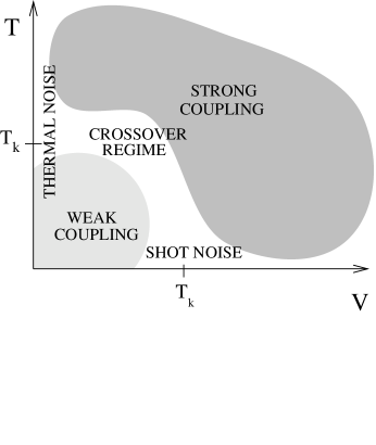
FIG. 7.: Phase diagram for $S_{I}$ and $S_{I_{b}}$. The strong coupling regime is characterized by either high temperature or high voltage values. The weak coupling regime corresponds to low temperature, low voltage values. $T_{k}$ is the energy scale that determines the crossover regime. Thermal and shot noise are characterized by the regions $T\gg V$ and $V\gg T$ respectively.

There are two interesting regimes: Thermal noise or $T\gg V$ and Shot noise or $V\gg T$.

• $T\gg V$ Thermal noise

  $$S_{I}=4g^{\prime}\frac{e^{2}}{2\pi}T-S_{I_{b}}=\cases{g^{\prime}\frac{e^{2}}{2\pi}\frac{4}{3}{\pi}^{2}T_{k}\left(\frac{T}{T_{k}}\right)^{3}&\mbox{$T_{k}\gg T$}\cr\cr 4g^{\prime}\frac{e^{2}}{2\pi}T-2g^{\prime}\frac{e^{2}}{2\pi}\pi T_{k}&\mbox{$T_{k}\ll T$}\cr}$$ (65)

• $V\gg T$ Shot noise

  $$S_{I}=S_{I_{b}}=\cases{g^{\prime}\frac{e^{2}}{2\pi}\frac{4}{3}T_{k}\left(\frac{eV}{2T_{k}}\right)^{3}&\mbox{$T_{k}\gg V$}\cr\cr 2g^{\prime}\frac{e^{2}}{2\pi}\pi T_{k}&\mbox{$T_{k}\ll V$}\cr}$$ (66)

(At $V=0$ the function $F_{1}=0$ and the limiting behavior of the function $F_{2}$ is calculated in appendix B.)

Furthermore, for $T_{k}\ll T$, $I_{b}\ll I$ (weak backscattering regime), and the expression for the noise in the current $I$ takes the form

$$S_{I}=4g^{\prime}\frac{e^{2}}{2\pi}T+2g^{\prime}\frac{e^{2}}{4\pi}\pi T_{k}\left[1-\frac{2}{\cosh^{2}\left(\frac{eV}{4T}\right)}\right]$$ (67)

From this expression, the crossover between thermal and shot noise can be studied. The crossover region is determined by the argument of the $\cosh(eV/4T)$ function. If the argument is written in the standard form of $(QV/2T)$, the value of $Q$ determined by this crossover corresponds to $Q=e/2$.

The backscattering current $I_{b}$ can also be calculated in this regime. Its expression reads:

$$I_{b}=\frac{e}{2\pi}\sqrt{\frac{g^{\prime}}{2}}T_{k}\pi\tanh\left(\frac{eV}{4T}\right)$$ (68)

After some algebra, the noise $S_{I}$ can be put in terms of the current $I_{b}$

$$S_{I}=4\,G\,T+2\left(\frac{e}{2}\right)I_{b}\tanh^{-1}\left(\frac{eV}{4T}\right)-4T\frac{dI_{b}}{dV}$$ (69)

where $G=dI/dV$ is the differential conductance of the junction. This expression has been obtained in previous works by Kane and Fisher [5] and Fendley and Saleur [7].

Further information can be obtained by comparing the limiting behavior of the noise in both, thermal and shot noise regime. In the strong coupling regime $T\gg T_{k}$ or $V\gg T_{k}$ the noise $S_{I_{b}}$ saturates to the same constant value for both cases, equilibrium ($V=0$) and non-equilibrium ($V\neq 0$). Notice that, while the saturation values of the noise $S_{I_{b}}$ both in the thermal and shot noise limits is determined by the (non-universal) energy scale $T_{k}$, their ratio takes the universal value

$$R_{I_{b}}={\frac{S_{I_{b}}(T=0;T_{k}\ll T)}{S_{I_{b}}(V=0;T_{k}\ll V)}}=1$$ (70)

Similarly, in the weak coupling regime $T_{k}\gg T$ or $T_{k}\gg V$, the noise $S_{I}$ vanishes as $(\frac{eV}{T_{k}})^{3}$ in the non-equilibrium regime ($V\neq 0$) and as $(\frac{T}{T_{k}})^{3}$ in the equilibrium one ($V=0$), as expected since the tunneling operator is irrelevant in the $\Gamma=0$ fixed point. Thus, the weak coupling regime can also be characterized by a ratio that is independent of the energy scale $T_{k}$. In this case, the ratio involves the noise $S_{I}$ in both the thermal and shot noise limits

$$R_{I}={\frac{S_{I}(T=0;T_{k}\gg T)}{S_{I}(V=0;T_{k}\gg V)}}=\frac{1}{8{\pi^{2}}}\left(\frac{eV}{T}\right)^{3}$$ (71)

It is worth to stress that while in the expression for $S_{I}$ and $S_{I_{b}}$, temperature and voltage play an analogous role, their physical meaning is quite different since in the $V=0,T\neq 0$ the system is in thermal equilibrium, while for $V\neq 0,T=0$ it is away from equilibrium.

VI Generalized Universal Noise Wilson Ratios

The ratios introduced above are interesting from the point of view of theory and experiment. These quantities are universal amplitude ratios of the behavior of the noise level at a given fixed point of the junction. They are a universal property of the fixed point. As such they are determined without a detailed knowledge of the crossover region. Hence, they can also be determined by a direct study of the behavior of the noise in the vicinity of the fixed point of interest, even for non-integrable systems. In particular, a perturbative analysis of the behavior of a generic $(\nu_{1},\nu_{2})$ junction can be used to calculate these ratios for a more general case. This is the purpose of this section.

Universal amplitude ratios are common in critical systems in general and in quantum impurity problems in particular. In the case of Kondo systems, the Wilson ratio, the ratio of the (suitably normalized) impurity paramagnetic susceptibility and of the slope of the impurity specific heat, describes the approach to the fixed point. The ratio defined in the last section bears an obvious similarity with the Wilson ratio.

Experimentally, both the thermal and shot noise can be measured, and therefore their ratio can be obtained and used to test the theoretical prediction based on the Luttinger liquid model for the edge states.

The asymptotic values of both the thermal and shot noise levels can be obtained, using perturbation theory, for a general junction $(\nu_{1},\nu_{2})$ through the value of the effective Luttinger parameter $g^{\prime}$. In the perturbative approach the expansion is done around a particular fixed point. For the weak coupling fixed point $\Gamma\rightarrow 0$ the current $I$ through the junction is small compared to the asymptotic large voltage current $I_{m}$. On the other hand, for the strong coupling $\Gamma\rightarrow\infty$, the backscattering current $I_{b}$ is small. Thus the ratios can be calculated in both cases by focusing on the appropriate small current. The duality relation between the two fixed points allows one to calculate the noise in both currents by simply taking $g^{\prime}$ into $1/g^{\prime}$.

  

The perturbative results are given by (see Ref. [9])

$$S_{I} = 2e^{2}|\Gamma|^{2}(2\pi T)^{\frac{2}{g^{\prime}}-1}\;B\left(\frac{1}{g^{\prime}}+i\frac{eV}{2\pi T},\frac{1}{g^{\prime}}-i\frac{eV}{2\pi T}\right)\cosh\left(\frac{eV}{2T}\right)$$ (72)

$$S_{I_{b}} = 2{e^{*}}^{2}|\tilde{\Gamma}|^{2}(2\pi T)^{2g^{\prime}-1}\;B\left(g^{\prime}+i\frac{e^{*}V}{2\pi T},g^{\prime}-i\frac{e^{*}V}{2\pi T}\right)\cosh\left(\frac{e^{*}V}{2T}\right)$$ (73)

where $e^{*}=g^{\prime}e$, the charge of the quasiparticle responsible for the noise in the weak backscattering limit.    

The shot to thermal noise ratios are then given by:

$$R_{I} = \frac{S_{I}(T\to 0)}{S_{I}(V\to 0)}=\frac{\pi}{\Gamma^{2}(1/g^{\prime})}\;\left(\frac{eV}{2\pi T}\right)^{2/g^{\prime}-1}$$ (74)

$$R_{I_{b}} = \frac{S_{I_{b}}(T\to 0)}{S_{I_{b}}(V\to 0)}=\frac{\pi}{\Gamma^{2}(g^{\prime})}\;\left(\frac{e^{*}V}{2\pi T}\right)^{2g^{\prime}-1}$$ (75)

In particular, for $g^{\prime}=1/2$, we obtain

$\displaystyle R_{I}=\frac{1}{8\pi^{2}}\left(\frac{eV}{T}\right)^{3}\qquad{\rm and}\qquad R_{I_{b}}=1$

which are the results obtained non-perturbatively in the previous section.

For a junction $(\frac{1}{3},\frac{1}{3})$ the effective Luttinger parameter $g^{\prime}=1/3$ and these ratios are

$$R_{I} = \frac{S_{I}(T\to 0)}{S_{I}(V\to 0)}=\frac{1}{128{\pi}^{4}}\left(\frac{eV}{T}\right)^{5}$$ (76)

$$R_{I_{b}} = \frac{S_{I_{b}}(T\to 0)}{S_{I_{b}}(V\to 0)}=\left[\frac{\pi(6\pi)^{\frac{1}{3}}}{\Gamma^{2}(\frac{1}{3})}\right]\left(\frac{T}{eV}\right)^{\frac{1}{3}}$$ (77)

Thus, these expressions could be compared with noise measurements in the geometries used by L. Saminadayar et. al [1] and by R. de Picciotto et. al[2] in the shot and thermal noise regimes.

These ratios are universal scaling functions in the sense that they are independent of the coupling constant ($\Gamma$ or $\tilde{\Gamma}$) or, alternatively, of the energy scale $T_{k}$. They still contain information on the Luttinger liquid behavior of the edge states which is manifest in the $V/T$ exponent and the $g^{\prime}$ dependent prefactor.

VII Auto-correlations in the incoming and outgoing branches

Thus far we have focused on the noise in the current flowing through the junction. More information can still be extracted from the noise by looking at correlations in the four branches involved in the scattering separately. In particular, the noise on both currents, $I$ and $I_{b}$, can be obtained from the measurements of correlations in a four probe setting, as done by L. Saminadayar et al. [1].

For this purpose, let us define the following auto and cross correlations between the densities in the various branches:

$$S_{ij}(\omega;x,y)\equiv\int_{-\infty}^{\infty}dt\;\cos\omega t\;\langle\{\rho_{i}(t,x),\rho_{j}(0,y)\}\rangle.$$ (78)

where the $i,j$ subscripts labels the branches $1,2$ (see Fig. 5). In this section we will focus primarily on the correlations for branches on the same side of the impurity ($x=y$). Consequently, we will work with

$$S^{\rm in\ }_{ij}(\omega) = S_{ij}(\omega;x,y)\quad{\rm for}\quad x=y<0$$ (79)

$$S^{\rm out}_{ij}(\omega) = S_{ij}(\omega;x,y)\quad{\rm for}\quad x=y>0$$ (80)

according to the side where the densities in consideration lie with respect to the impurity. Whenever we wish to address a general property of the noise valid in either case, we shall also drop the superscripts $out$ and $in$, and simply use $S_{ij}$.

Just as in the case of $S_{I}(\omega)$ defined in Eq. (26), the related quantities defined in Eqs. (78-80) are also functions of the tunneling amplitude $\Gamma$, the voltage $V$ and the temperature $T$. Besides the separation between an equilibrium $S^{\rm eq}$ and an excess $S^{\rm ex}$ contribution to the noise, we can alternatively also separate the noise into an impurity contribution $S^{\rm imp}$, and the contribution of the two decoupled channels, $S^{\Gamma=0}$. This separation of physical quantities is standard in quantum impurity problems. $S^{\rm imp}$ and $S^{\Gamma=0}$ are simply related to quantities easily calculable in the basis of the fields ${\tilde{\phi}}_{+,-}$. Since these fields are decoupled from each other, we only need to calculate their auto-correlation functions. The field ${\tilde{\phi}}_{+}$ is a free field, and its noise spectrum at zero temperature can be calculated in a straightforward way giving:

$$S_{+}(\omega)={\frac{e^{2}}{2\pi}}|\omega|\coth{\frac{|\omega|}{2T}}$$ (81)

The noise spectrum for the field ${\tilde{\phi}}_{-}$ is defined similarly as above to be:

$$S_{-}(\omega;x,y)=\int_{-\infty}^{\infty}dt\;\cos\omega t\;\langle\{\rho_{-}(t,x),\rho_{-}(0,y)\}\rangle.$$ (82)

Below, we give explicit relations between $S_{\pm}(\omega)$ and the noise expressions $S^{\rm imp}$ and $S^{\Gamma=0}$ for the incoming and outgoing branches.

The noise in the original branches can be related to the noise in the rotated branches, as follows. We begin by utilizing the generalization of Eq. (12) for two filling fractions $\nu_{1}$ and $\nu_{2}$:

$$\left(\matrix{\rho_{1}\cr\rho_{2}}\right)=\frac{1}{2}\;\left(\matrix{\sqrt{\frac{\nu_{1}}{\nu_{2}}}+1&\sqrt{\frac{\nu_{1}}{\nu_{2}}}-1\cr\sqrt{\frac{\nu_{2}}{\nu_{1}}}-1&\sqrt{\frac{\nu_{2}}{\nu_{1}}}+1}\right)\left(\matrix{\rho^{\prime}_{1}\cr\rho^{\prime}_{2}}\right)\ .$$ (83)

In order to calculate the noise spectrum of this junction we use Eq. (78). The noise, or density, correlations in the two problems can also be related through the matrix in Eq. (83). It suffices to look at $S_{11}$, since the results are analogous for $S_{22}$.

$$S_{11}=\frac{1}{2}\left[\left(\frac{\nu_{1}}{\nu_{2}}+1\right)\;S^{\prime}_{11}+\left(\frac{\nu_{1}}{\nu_{2}}-1\right)\;S^{\prime}_{12}\right]\ \ ,$$ (84)

where we used that $S^{\prime}_{11}=S^{\prime}_{22}$ and $S^{\prime}_{12}=S^{\prime}_{21}$.

Now we need a relationship between $S^{\prime}_{12}$ and $S^{\prime}_{11}$, which we obtain by rotating to the decoupled $\phi_{\pm}$ fields as in Eq. (15) (which we repeat below for completeness; see also Fig. 4):

$$\left(\matrix{\rho^{\prime}_{1}\cr\rho^{\prime}_{2}}\right)=\sqrt{\frac{g^{\prime}}{2}}\left(\matrix{1&1\cr 1&-1}\right)\left(\matrix{\rho_{+}\cr\rho_{-}}\right)\ \ .$$ (85)

We can write

$$S^{\prime}_{11} = \frac{g^{\prime}}{2}\left(S_{+}+S_{-}\right)$$ (86)

$$S^{\prime}_{12} = \frac{g^{\prime}}{2}\left(S_{+}-S_{-}\right)=\frac{g^{\prime}}{2}\left(2S_{+}\right)-\frac{g^{\prime}}{2}\left(S_{+}+S_{-}\right)$$ (87)

$$= S^{\prime\Gamma=0}_{11}-S^{\prime}_{11}\ \ .$$ (88)

We have used in the last line above the fact that, at $\Gamma=0$, $S_{-}=S_{+}$. Thus, one can cast one of the terms as $S^{\prime\Gamma=0}_{11}$. Using this relationship between $S^{\prime}_{12}$ and $S^{\prime}_{11}$ in Eq. (84) we obtain

$$S_{11}=S^{\prime}_{11}+\frac{1}{2}\left(\frac{\nu_{1}}{\nu_{2}}-1\right)S^{\prime\Gamma=0}_{11}\$$ (89)

which is equivalent, upon separating decoupled and impurity components of the noise, to

$$S^{\Gamma=0}_{11} = \frac{1}{2}\left(\frac{\nu_{1}}{\nu_{2}}+1\right)S^{\prime\Gamma=0}_{11}$$ (90)

$$= \frac{1}{2}\left(\frac{\nu_{1}}{\nu_{2}}+1\right)g^{\prime}{\frac{e^{2}}{2\pi}}|\omega|\coth{\frac{|\omega|}{2T}}$$ (91)

$$= \nu_{1}{\frac{e^{2}}{2\pi}}|\omega|\coth{\frac{|\omega|}{2T}}$$ (92)

and

$$S^{\rm imp}_{11}=S^{\prime\rm imp}_{11}\$$ (93)

It is important to observe this distinct behavior for the decoupled and impurity components of the noise. The important result to be extracted from Eqs. (92-93) is that

1. The noise in the current of each branch, in the $\Gamma=0$ limit, depends only on the filling fractions $\nu_{1},\nu_{2}$ on either side of the junction, and as such it scales with the conductances.

2. The impurity contribution to the noise $S^{\rm imp}$ is exactly the same as for the rotated basis, with an effective $g^{\prime}$ given by the harmonic average of $\nu_{1}$ and $\nu_{2}$. $S^{\rm imp}$ depends on the combined properties of the coupled system.

Let us consider now the behavior of the noise in the different branches.

A Noise in the Incoming Channels

We will focus primarily on the auto-correlations of the densities on the FQH and the Fermi Liquid (FL) sides of the junction, so it is useful to introduce an explicit notation

$\displaystyle S^{\rm\ in}_{\rm FQH}=S^{\rm in}_{11}\qquad{\rm and}\qquad S^{\rm in}_{\rm FL}=S^{\rm in}_{22}$

More explicitly, these correlations can be written in terms of the densities and the definitions in Eqs. (78,79): given by:

$$S^{\rm\ in}_{\rm FQH} = \int_{-\infty}^{\infty}dt\;\cos\omega t\;\langle\{\rho_{1}(x<0,t),\rho_{1}(x<0,0)\}\rangle$$ (94)

$$S^{\rm in}_{\rm FL} = \int_{-\infty}^{\infty}dt\;\cos\omega t\;\langle\{\rho_{2}(x<0,t),\rho_{2}(x<0,0)\}\rangle$$ (95)

Using Eqs.(12) and (15), the densities $\rho_{1,2}$ can be written in terms of the densities of the fields ${\tilde{\phi}}_{+,-}$:

$$\rho_{1}(x<0,t) = \sqrt{\frac{g^{\prime}\nu}{2}}{\tilde{\rho}}_{+}(x<0,t)+\sqrt{\frac{g^{\prime}}{2}}{\tilde{\rho}}_{-}(x<0,t)$$ (97)

$$\rho_{2}(x<0,t) = \sqrt{\frac{g^{\prime}}{2\nu}}{\tilde{\rho}}_{+}(x<0,t)-\sqrt{\frac{g^{\prime}}{2}}{\tilde{\rho}}_{-}(x<0,t)$$ (98)

The noise in the incoming channels is then reduced to a sum of two terms, one involving the noise in the field ${\tilde{\rho}}_{+}$ and the other involving the noise in the field ${\tilde{\rho}}_{-}$. As mentioned in the previous section, the field ${\tilde{\rho}}_{+}$ is free and its noise is given by Eq.(81). For the noise in the field ${\tilde{\rho}}_{-}$ for $x<0$ we use Eqs. (34- 43) to obtain:

$$S_{-}(\omega,x<0)={\frac{e^{2}}{2\pi}}|\omega|\coth{\frac{|\omega|}{2T}}$$ (100)

Using the fact that $\langle{\tilde{\rho}}_{+}{\tilde{\rho}}_{-}\rangle=0$ and Eqs.(81, 100) we find:

$$S^{\rm\ in}_{\rm FQH} = \nu{\frac{e^{2}}{2\pi}}|\omega|\coth{\frac{|\omega|}{2T}}$$ (101)

$$S^{\rm in}_{\rm FL} = {\frac{e^{2}}{2\pi}}|\omega|\coth{\frac{|\omega|}{2T}}$$ (102)

These results agree with results obtained in Ref. [10] for the incoming branches as expected. The incoming branches are insensitive to the tunneling between the edges as a result of their chirality.

B Noise in the Outgoing Channels

Again, we will focus primarily on the auto-correlations of the densities on the FQH and the Fermi Liquid (FL) sides of the junction, and so we introduce an explicit notation

$\displaystyle S^{\rm\ out}_{\rm FQH}=S^{\rm out}_{11}\qquad{\rm and}\qquad S^{\rm out}_{\rm FL}=S^{\rm out}_{22}$

The expressions for the noise in the outgoing channels are given by:

$$S^{\rm\ out}_{\rm FQH} = \int_{-\infty}^{\infty}dt\;\cos\omega t\;\langle\{\rho_{1}(x>0,t),\rho_{1}(x>0,0)\}\rangle$$ (103)

$$S^{\rm out}_{\rm FL} = \int_{-\infty}^{\infty}dt\;\cos\omega t\;\langle\{\rho_{2}(x>0,t),\rho_{2}(x>0,0)\}\rangle$$ (104)

In order to write the densities $\rho_{1}(x>0,t)$ and $\rho_{2}(x>0,t)$ in terms of ${\tilde{\rho}}_{+,-}$, we use Eqs.(15) and (22):

$$\rho_{1}(x>0,t) = \sqrt{\frac{g^{\prime}\nu}{2}}{\tilde{\rho}}_{+}(x>0,t)-\sqrt{\frac{g^{\prime}}{2}}{\tilde{\rho}}_{-}(x>0,t)$$ (106)

$$\rho_{2}(x>0,t) = \sqrt{\frac{g^{\prime}}{2\nu}}{\tilde{\rho}}_{+}(x>0,t)+\sqrt{\frac{g^{\prime}}{2}}{\tilde{\rho}}_{-}(x>0,t)$$ (107)

As we have done previously when discussing the noise in the current $I$, we will express the noise in the incoming and outgoing channels in terms of $T_{k}$, the temperature $T$, the frequency $\omega$, and the voltage $V$, through the Josephson frequency $\omega_{0}=eV$ (in units with $\hbar=1$). After some algebra we find,

$$S^{\rm\ out}_{\rm FQH} = \nu{\frac{e^{2}}{2\pi}}|\omega|\coth{\frac{|\omega|}{2T}}+S^{\rm imp}\left(\omega,V,T,T_{k}\right)$$ (109)

$$S^{\rm out}_{\rm FL} = {\frac{e^{2}}{2\pi}}|\omega|\coth{\frac{|\omega|}{2T}}\ +S^{\rm imp}\left(\omega,V,T,T_{k}\right)$$ (110)

  

where

$$S^{\rm imp} = \frac{T_{k}}{2\pi}\int_{-\infty}^{\infty}dx\left\{\frac{x(2x-\omega/T_{k})}{(x^{2}+1)[(x-\omega/T_{k})^{2}+1]}\left[n_{T_{k}x-\omega}\;n_{-T_{k}x}+(1-n_{\omega-T_{k}x)})(1-n_{T_{k}x})\right]+(\omega\to-\omega)\right\}$$ (111)

$$- \frac{T_{k}}{2\pi}\int_{-\infty}^{\infty}dx\left\{\frac{4x(x-\omega/T_{k})+(\omega/T_{k})^{2}}{(x^{2}+1)[(x-\omega/T_{k})^{2}+1]}n_{T_{k}x-\omega}(1-n_{T_{k}x})+(\omega\to-\omega)\right\}$$ (112)

and

$$n_{T_{k}x}=\frac{1}{1+e^{T_{k}/T(x-eV/2T_{k})}}$$ (113)

   

One can show that the expressions in Eq. (53) for the noise in the current through the barrier $I$ and Eq. (112) coincide in the limit of $T=0$. For non-zero temperatures, cross correlations between $in$ and $out$ branches that appear in the expression for the noise in the current $I$ Eq. (51) make the results no longer equal.

VIII Conclusions

In this paper we have discussed the noise spectrum of generic tunnel junctions between FQH systems at inequivalent Laughlin filling fractions $\nu_{1}$ and $\nu_{2}$, and discussed in great detail the special exactly solvable case of a junction between the $\nu=1/3$ state and a normal metal (i. e., $\nu=1$). The main focus of this work was to obtain the expression for the DC noise of the current $I$ through the ($\nu_{1},\nu_{2}$) junction in order to determine the charge of the carriers. Using the single point contact model developed in Ref. [12, 14] and a suitable set of transformations, we mapped the original model into an effective model of a junction between equivalent FQH states at certain filling fractions. This effective model possesses an exact duality transformation between weak and strong tunneling amplitudes.

We found that different equivalent descriptions can be used to picture the physics of noise in these junctions. In one picture, more transparent in the weak tunneling or strong backscattering regime, the shot noise is produced by electrons, which are the natural common excitations of the decoupled system, tunneling through the junction. In contrast, in the weak backscattering or strong tunneling limit, we obtained a quite interesting result. We found that the level of DC shot noise can be attributed to the tunneling of a fractionally charged state whose charge does not coincide with the charges of the quasiparticles of the isolated Laughlin states on either side of the junction. Instead, the fractionally charged state governing the tunneling properties in this regime can be best regarded as a soliton of the coupled system. The charge of the solitons is, in units of the electron charge, the harmonic average of the filling fractions of the two Laughlin states. Furthermore, as pictured in Fig. 3, the same soliton states (and hence the same conductance) arise in all junctions between Laughlin states with the same harmonic mean. Therefore, any two-terminal measurement of these junctions cannot distinguish one from another and, consequently, have no means of determining uniquely the quantum numbers of the quasiparticles of the bulk Laughlin states of the junction.

The feature that the noise level tracks the saturation differential conductance is a general property of QPCs between Laughlin states. Thus, the only way to tell if the shot noise level is a measurement of the fractional charge of a state or if instead is a measurement of the differential conductance is to carry out noise experiments in fractions which are not in the Laughlin sequence. For example, for $\nu={\frac{2}{5}}$, the charge is ${\frac{1}{5}}$.

The special case of $(1,{\frac{1}{3}})$ can be exactly solved by a further mapping to an equivalent free fermion system. For this case, of direct physical interest, we calculated exactly the current correlation functions of the original junction in terms of the correlation functions of the fermions. We examined the DC noise in both the current $I$ and the backscattering current $I_{b}$ at zero and finite temperature and for all voltages. We present our results in the form of a phase diagram in the voltage-temperature plane. This description treats (non-equilibrium) shot noise and thermal noise on the same footing. We showed that there is a natural generalization of Wilson ratios, which we defined as quotients between the shot noise and the thermal noise levels for both currents $I$ and $I_{b}$. These are universal amplitude ratios, they are scaling functions of $V/T$ independent of the coupling constant near the weak and strong coupling fixed points, and are related by duality. These ratios can be used to analyze the experimental data in the recent works by L. Saminadayar et. al. [1] and R. de Picciotto et. al. [2] for both limits of thermal and shot noise in a unified way.

We also discuss a four probe geometry that allows for the extraction of more information from noise measurements by looking at the auto-correlations of the density or current fluctuations on the incoming and outgoing channels at the junction. In section VII we discuss a four probe geometry and calculate the noise in all four channels. As a consequence of chirality, the noise in the incoming channels is insensitive to the presence of the QPC, and it is given by the Johnson-Nyquist noise level, which is proportional to the conductance determined by the respective filling fraction in either side of the junction. In contrast, the noise in the outgoing channels contains the information on the tunneling coupling, and depends on both filling fractions $\nu_{1}$ and $\nu_{2}$.

We finalize by proposing an experimental setup that can test our results. The geometry that we believe is most promising is depicted in the Fig. 2. This setup is a variant of the cleaved edge overgrowth used by A. Chang and collaborators [3, 4]. The only (and important) difference is that the tunneling region where the barrier is significantly lower is sufficiently narrow to be regarded as a QPC. In practice, for a smooth barrier, a tunneling region a few cyclotron lengths wide should be sufficient to produce a few coherent tunneling centers. In fact, many of the predictions of references [12, 14] can also be tested in this QPCs.

IX Acknowledgments

This work has been supported by the National Science Foundation through the Grant NSF DMR-94-24511, by a fellowship of the University of Illinois and by the Science and Technology Center for Superconductivity of the University of Illinois (NPS). We are grateful to A.  Chang, C. Glattli, M.  Grayson and M. Reznikov for many insightful comments and discussions.

A Calculation of the functions $F_{1}$ and $F_{2}$

In this appendix we evaluate the integrals $F_{1}$ and $F_{2}$ used for calculating the noise in Sec. V. The strategy is to use the complex plane and several identities involving the $\psi$ function (logarithmic derivative of the $\Gamma$ function). First we will evaluate $F_{1}$ given by

$$F_{1} = \sinh\left(\frac{V}{2T}\right)\;\;\;\int_{-\infty}^{\infty}dx\;\;\;f(x)$$ (A1)

$$f(x) = \frac{x^{2}}{(1+x^{2})^{2}}\;\frac{\tanh\left(\frac{V}{4T}-\frac{T_{k}x}{2T}\right)}{\cosh\left(\frac{T_{k}x}{2T}+\frac{V}{4T}\right)\cosh\left(\frac{T_{k}x}{2T}-\frac{V}{4T}\right)}$$ (A2)

To simplify the notation we introduce $a=(1/2)T_{k}/T$ and $b=(1/4)V/T$. After a few algebraic manipulations the integral is cast in the form:

$$F_{1} = \frac{a}{2}\sinh^{2}(2b)\;\;\;\int_{-\infty}^{\infty}dy\;\;\;f(y)$$ (A3)

$$f(y) = \frac{y^{2}}{(a^{2}+y^{2})^{2}}\;\;\frac{1}{\cosh^{2}(y+b)\cosh^{2}(y-b)}$$ (A4)

It is straightforward to show that $F_{1}$ can be calculated by complex variable methods. The integrand has double poles at $z_{\circ}=\pm ia$ and at $z_{n}=\pm b+i\pi(n+1/2)$ and $z_{n}=\pm b-i\pi(n+1/2)$. Because the integral is on the real axis from $-\infty$ to $\infty$ it is enough to consider the contribution from the poles in the upper (or lower) complex plane. After some calculations it can be shown that $F_{1}$ is given by

$$F_{1}=\frac{\pi}{4}\sinh^{2}(2b)\frac{1+2a[\tan(a-ib)+\tan(a+ib)]}{\cos^{2}(a+ib)\cos^{2}(a-ib)}$$ (A5)

$$-\frac{2i\pi a}{\tanh(2b)}\sum_{n=0}^{\infty}\Biggl{\{}\frac{[b+i\pi(n+1/2)]^{2}}{\bigl{[}a^{2}+\bigl{(}b+i\pi(n+1/2)\bigr{)}^{2}\bigr{]}^{2}}-(b\rightarrow-b)\Biggr{\}}$$ (A6)

$$-2i\pi a\sum_{n=0}^{\infty}\Biggl{\{}\frac{\bigl{[}b+i\pi(n+1/2)\bigr{]}\bigl{[}\bigl{(}b+i\pi(n+1/2)\bigr{)}^{2}-a^{2}\bigr{]}}{\bigl{[}a^{2}+\bigl{(}b+i\pi(n+1/2)\bigr{)}^{2}\bigr{]}^{3}}$$ (A7)

$$+\;(b\rightarrow-b)\Biggr{\}}$$ (A8)

To further simplify this expression we introduce the function $S(a,b)$ as

$$S(a,b)=\sum_{n=0}^{\infty}\frac{1}{a^{2}+[b+i\pi(n+1/2)]^{2}}$$ (A9)

In terms of $S(a,b)$ the function $F_{1}$ is given by:

$$F_{1}=\frac{\pi}{4}\sinh^{2}(2b)\frac{1+2a[\tan(a+ib)+\tan(a-ib)]}{\cos^{2}(a+ib)\cos^{2}(a-ib)}$$ (A10)

$$-\;\frac{2i\pi a}{\tanh(2b)}\Biggl{\{}S(a,b)+\frac{a}{2}\frac{\partial}{\partial a}S(a,b)-c.c.\Biggr{\}}$$ (A11)

$$+\;\pi ia\frac{\partial}{\partial b}\Biggl{\{}S(a,b)+\frac{a}{2}\frac{\partial}{\partial a}S(a,b)-c.c.\Biggr{\}}$$ (A12)

The $S(a,b)$ function can be related to the $\psi$-function (digamma) as follows:

$$S(a,b)=\frac{1}{2\pi a}\left[\psi\left(\frac{1}{2}-\frac{a+ib}{\pi}\right)-\psi\left(\frac{1}{2}+\frac{a-ib}{\pi}\right)\right]$$ (A13)

By defining $\pi z=a+ib$ we find that $F_{1}$ is given by:

$$F_{1}=\frac{\pi}{4}\sinh^{2}(2b)\frac{1+2a[\tan(\pi z)+\tan(\pi\bar{z})]}{\cos^{2}(\pi z)\cos^{2}(\pi\bar{z})}$$ (A14)

$$-\frac{i}{2\tanh(2b)}\Biggl{\{}\frac{a}{\pi}\left[\psi^{{}^{\prime}}(1/2+z)-\psi^{{}^{\prime}}(1/2-z)-(z\rightarrow\bar{z})\right]$$ (A15)

$$+\psi(1/2+z)+\psi(1/2-z)-(z\rightarrow\bar{z})\Biggr{\}}$$ (A16)

$$+\frac{1}{4\pi}\Biggl{\{}\psi^{{}^{\prime}}(1/2-z)-\psi^{{}^{\prime}}(1/2+z)-(z\rightarrow\bar{z})$$ (A17)

$$-\frac{a}{\pi}\left[\psi^{{}^{\prime\prime}}(1/2+z)+\psi^{{}^{\prime\prime}}(1/2-z)+(z\rightarrow\bar{z})\right]\Biggr{\}}$$ (A18)

where $\psi^{{}^{\prime}}(z)$ and $\psi^{{}^{\prime\prime}}(z)$ are the first and second derivatives of the $\psi$ function with respect to their arguments, evaluated at $z$.

The calculation of $F_{2}$ and $F_{3}$ follows similar steps. Thus, for the particular case of the $(1,\frac{1}{3})$ junction, we find that the scaling functions $F_{1}$, $F_{2}$ and $F_{3}$, which describe the crossover from weak to strong coupling, are determined by a single meromorphic function, the digamma function, and its derivatives, evaluated at $\left({\frac{T_{k}}{2T}}\pm i{\frac{eV}{4T}}\right)$. The behavior of these correlation functions, which describe non-equilibrium properties, is remarkably reminiscent of the analytic properties of thermodynamic functions of integrable quantum impurity problems discovered recently by Fendley et. al[6, 7].

B Limiting behavior of $F_{2}$ at $V=0$

We calculate explicitly the expressions appearing in Sec. V for the function $F_{2}$ at zero voltage in both regimes: $T_{k}\gg T$ and $T_{k}\ll T$. The expression for $F_{2}$ at finite voltage and temperature is given by:

$$F_{2}=i\frac{\partial}{\partial b}\left\{\psi\left(\frac{1}{2}+\frac{a-ib}{\pi}\right)-\psi\left(\frac{1}{2}+\frac{a+ib}{\pi}\right)\right\}$$ (B1)

where $a=(1/2)T_{k}/T$ and $b=(1/4)V/T$. After taking the derivatives

$$F_{2}=\frac{1}{\pi}\left[\psi^{{}^{\prime}}\left(\frac{1}{2}+\frac{a-ib}{\pi}\right)+\psi^{{}^{\prime}}\left(\frac{1}{2}+\frac{a+ib}{\pi}\right)\right]$$ (B2)

At zero voltage $b=0$ and the expression for $F_{2}$ reduces to

$$F_{2}=\frac{2}{\pi}\psi^{{}^{\prime}}\left(\frac{1}{2}+\frac{T_{k}}{2\pi T}\right)$$ (B3)

For $T_{k}\ll T$ the leading order in $F_{2}$ is simply

$$F_{2}=\frac{2}{\pi}\psi^{{}^{\prime}}\left(\frac{1}{2}\right)=\pi$$ (B4)

For $T_{k}\gg T$ we need to use some relations among $\psi-$ functions with different arguments:

$$\psi^{{}^{\prime}}\left(\frac{1}{2}+z\right) = 4\psi^{{}^{\prime}}(1+2z)-\psi^{{}^{\prime}}(1+z)$$ (B5)

$$\psi^{{}^{\prime}}(1+z) = \psi^{{}^{\prime}}(z)-\frac{1}{z^{2}}$$ (B6)

Finally, we use the asymptotic expansions for the $\psi$ function for large values of its argument to get

$$F_{2}=\frac{4T}{T_{k}}-\frac{4{\pi}^{2}}{3}\left(\frac{T}{T_{k}}\right)^{3}+{\cal O}\left(\frac{T}{T_{k}}\right)^{4}$$ (B7)

REFERENCES

- [1] L. Saminadayar, D. C. Glattli, Y. Jin and B. Etienne, Phys. Rev. Lett. 79, 2526 (1997).
- [2] R. de Picciotto, M. Reznikov, M. Heiblum, V. Umansky, G. Bunin and D. Mahalu, Nature 389, 162 (1997).
- [3] A. M. Chang, L. N. Pfeiffer, and K. W. West, Phys. Rev. Lett. 77, 2538 (1996).
- [4] M. Grayson, D. C. Tsui, L. N. Pfeiffer, K. W. West and A. M. Chang, Phys. Rev. Lett. 80, 1062 (1998).
- [5] C. L. Kane, and M. P. A. Fisher, Phys. Rev. Lett. 72, 724 (1994).
- [6] P. Fendley, A. W. W. Ludwig and H. Saleur, Phys. Rev. Lett. 75, 2196 (1995).
- [7] P. Fendley and H. Saleur, Phys. Rev. B 54, 10845 (1996).
- [8] F. Lesage and H. Saleur, Nuc. Phys. B 493, 613 (1997).
- [9] C. de C. Chamon, D. E. Freed, and X. G. Wen, Phys. Rev. B 51, 2363 (1995).
- [10] C. de C. Chamon, D. E. Freed, and X. G. Wen, Phys. Rev. B 53 4033, (1996) and references therein.
- [11] C. L. Kane, and M. P. A. Fisher, Phys. Rev. B 46, 15233 (1992).
- [12] C. de C. Chamon and Eduardo Fradkin, Phys. Rev. B 56, 2012 (1997).
- [13] For a review see, X. G. Wen, Adv. in Phys. 44,405 (1995).
- [14] Nancy P. Sandler, Claudio de C. Chamon, and Eduardo Fradkin. To appear in Phys. Rev. B, May 15 (1998).
- [15] X. G. Wen, Phys. Rev. B 41, 12838 (1990).
- [16] N. Andrei, K. Furuya, and J. H. Lowenstein, Rev. Mod. Phys. 55, 331 (1983).