Maxwell Equations and Irreversibility

Abstract

Two questions connected to the macroscopic Maxwell equations are addressed: First, which form do they assume in the hydrodynamic regime, for low frequencies, strong dissipation and arbitrary field strengths. Second, what does this tell us about irreversibility and coarse-grained description.

Contents

toc

I Introduction

You are probably ambivalent toward the article you have just started to read, or even harbor dark suspicions about it. These feelings are admittedly hard to avoid when encountering someone purporting to reveal news about the centenarian Maxwell equations. Afterall, we know all there is to know about the Maxwell equations, do we not? Well, no, we do not. Despite the impression we came away with from various courses on electrodynamics, there are large gaps in our understanding on this subject, and the most glaring ones deal with the connection between electrodynamics and thermodynamics. These two independently developed classical areas of physics apparently do not mix well: Jackson (1975) does not mention entropy in his classic book at all, while Callen (1985) has eliminated the (partly erroneous) chapter on magnetic and electric system in the second edition of his definitive work.

Nevertheless, it must be sensible to ask questions such as when an electromagnetic field configuration is in equilibrium, and how this equilibrium state is arrived at. Equilibrium fields are the ones that maximize the entropy, is there a simple equation expressing this property? Equilibrium fields are always static, but is it possible, in dielectrics, for a static field to be off-equilibrium? These are some of the questions answered below, and we go on from these answers to understand how field dissipation can be accounted for in dynamic situations, for a general system of nonlinear constitutive relations – where postulating imaginary parts for the permeabilities $\varepsilon$ and $\mu$ fails to work. We also go on to understand what the electromagnetic force is that a polarizable and magnetizable body feels – both in and off equilibrium. Fortunately, all these results are fairly simple and universal, and in fact quite suitable for being introduced into a university course on “electrodynamics in continua”.

In section II, I shall summarize the state of the art of the Maxwell equations as it is conventionally treated, and point out the extent of securely understood physics. Starting with section III, a different approach, that of the thermo- and hydrodynamic theory, is introduced. The hydrodynamic theory, the response of dense and dissipative systems exposed to slowly varying external fields of nonlinear strength, is discussed in section V. Interspersed between these considerations, I shall often stop to deliberate over two fundamental aspects of macroscopic theories — coarse-grained description and irreversibility — starting right at the beginning of the next section, but mainly in section VI. The difference between the hydrodynamic and the linear response theory is dwelt on in section VII, with some surprising and instructive results. Finally, in section VIII, the old but confusing subject about the electromagnetic force in a coarse-grained description is considered and clarified.

[Arguments that are not usually reproduced in a seminar, only invoked when the appropriate question is raised, are given – as here – in large square brackets. They may be skipped on first reading.]

II Less Accurate Is More Difficult?

The actual difference between the electrodynamics in vacuum and continua is one of accuracy, better: one of resolution. Denoting the grain size of descriptive grid as $\xi$, and the average distance between the charge carriers as $d$, the vacuum Maxwell equations as a high resolution theory are valid for $d\gg\xi$. Since the input, the density of charge and current, is in principle arbitrarily accurate, we are able to calculate the fields ${\bf e}$ and ${\bf b}$ to any desired resolution.

Their contribution to the energy, and the Lorentz force are, respectively

$$u^{\rm em}=\textstyle\frac{1}{2}(\varepsilon_{0}e^{2}+b^{2}/\mu_{0}),\quad{\bf f}=\varrho_{e}({\bf e}+\mbox{\boldmath$v$}\times{\bf b}).$$ (1)

In conjunction with the Newtonian equation of motion, these two expressions account for the feedback, for how the field affects the motion of the material. So we have at our disposal a closed theory — a classical one with a known quantum mechanical generalization — that is conceptually simple yet technically intractable for dense systems.

The circumstances are reversed if we check our ambition and seek enlightment from a low-resolution theory, $d\ll\xi$: The technical difficulties are greatly reduced, but conceptually we enter murky waters.

Because the density of charge $\langle\varrho_{e}\rangle$ and current $\langle j_{e}\rangle=\langle\varrho_{e}v\rangle$, are now spatially averaged quantities, we must deal with hidden charges and currents, making it necessary to consider four instead of two fields: ${\bf D}$, ${\bf B}$, ${\bf E}^{M}$, and ${\bf H}^{M}$ — all coarse-grained, hence in capital letters. (As will become clear soon, we need to distinguish ${\bf E}^{M}$, ${\bf H}^{M}$ from ${\bf E}$, ${\bf H}$. The former two are the usual fields as defined by the Maxwell equations; the latter two will be introduced later.) Given constitutive relations, linear if the field is sufficiently weak,

$${\bf D}=(\varepsilon^{\prime}+i\varepsilon^{\prime\prime}){\bf E}^{M},\quad{\bf B}=(\mu^{\prime}+i\mu^{\prime\prime}){\bf H}^{M},$$ (2)

we are again able to calculate the field from the source. The real parts of the permeabilities, $\varepsilon^{\prime}$ and $\mu^{\prime}$, account for the reactive responses such as the oscillatory motion of hidden charges; the imaginary parts, $\varepsilon^{\prime\prime}$ and $\mu^{\prime\prime}$, parametrize dissipation and absorption. If a field is stronger, it is customary to take the corresponding permeability again as a function of the field. But one goes beyond linear response only at the price of loosing all the simple relations, especially the identification of the imaginary part with dissipation.

Deplorable as this is, the problems are worse for the feedback, the effect of the field on the motion of the material. The reason is that both the electromagnetic energy and the Lorentz force, Eqs(1), are nonlinear. And the knowledge of the coarse-grained quantities $\langle\varrho_{e}\rangle$, $\langle{\bf j}_{e}\rangle$, ${\bf E}^{M}=\langle{\bf e}\rangle$, ${\bf B}=\langle{\bf b}\rangle\dots$ is quite useless if we need to know the values of $\langle\varrho_{e}{\bf e}\rangle$, or $\langle\varrho_{e}\mbox{\boldmath$v$}\times{\bf b}\rangle$. Nevertheless, bold souls, without much ado, simply write

$$\rho{\textstyle\frac{\rm d}{{\rm d}t}}v_{i}+\nabla_{i}P+\nabla_{j}\pi^{D}_{ij}=\left[\langle\varrho_{e}\rangle{\bf E}^{M}+\langle{\bf j_{e}}\rangle\times{\bf B}\right]_{i}.$$ (3)

In the absence of fields, the right side of Eq(3) is zero, and what remains is the Navier-Stokes equation, an expression of momentum conservation in the low-resolution, hydrodynamic physics: Both the pressure $P$, a quintessentially thermodynamic quantity, and the viscous stress tensor $\pi^{D}_{ij}$, a dissipative term, presume an infinitesimal volume element that contain enough particles to form a system in local equilibrium. This volume element is nothing but the descriptive grain, of the size $\xi^{3}$, we therefore have $d\ll\xi$. Now, any theory, and each equation, must consistently have a unique resolution. So the sources and fields on the right hand side must not be of high resolution, but it is not at all clear that the expression as written, in low-resolution quantities, is correct. Needless to say, anyone employing this fairly popular equation, or a variant of it, bears the burden of proof for its validity. [An example of a system in which Eq(3) does hold is a weakly dissociated gas, where the density of charge carriers is much lower than the density of neutral particles. Assuming negligible dipole moments for the latter, we have two interparticle distances, $d_{n}$ for neutral particles, and $d_{e}$ for the charge carriers. Then the resolution of this equation may be chosen as $d_{n}\ll\xi\ll d_{e}$, such that it is of low-resolution for the neutral particles, yet of high resolution for the charge carriers.]

Actually, things are not as bleak as they seem right now, and a few lesser known results do considerably brighten up the prospect of formulating the feedback, and closing the low-resolution Maxwell theory. These results are (i) the thermodynamics of the electromagnetic field and (ii) the expressions for the energy and stress tensor at finite frequencies, albeit without dissipation. They will be briefly outlined in the next section and are taken from the one good book on this subject, Volume VIII of Landau and Lifshitz (1984), referred to below as LL8; see also Kentwell and Jones (1987) for a nice review of the state of the art. The thermodynamic considerations as presented, however, contain enough generalization and shifts in interpretation, from the unfortunately brief treatment in §18 of LL8, that I most probably have to bear the blame if you should find faults in any statements here.

III The Thermodynamics of Fields

We start from the energy density $u$ in the system’s rest frame, as a function of the entropy density $s$, mass density $\rho$, and the two fields ${\bf D}$ and ${\bf B}$,

$${\rm d}u=T{\rm d}s+\mu{\rm d}\rho+{\bf E}\cdot{\rm d}{\bf D}+{\bf H}\cdot{\rm d}{\bf B}.$$ (4)

Being defined as $\partial u/\partial{\bf D}$ and $\partial u/\partial{\bf B}$, respectively, ${\bf E}$ and ${\bf H}$ are (like $T\equiv\partial u/\partial s$) functions of all the thermodynamic variables. For weak fields (and barring ferroelectricity or ferromagnetism), an expansion yields

$${\bf E}={\bf D}/\bar{\varepsilon},\quad{\bf H}={\bf B}/\bar{\mu},$$ (5)

where $\bar{\varepsilon}$ and $\bar{\mu}$ may be functions of temperature and density, but not the frequency.

Maximizing the entropy $S=\int\!dVs$ for a stationary dielectric medium, with the constraints of constant energy, constant mass, and the validity of the two non-temporal Maxwell equations, $\nabla\cdot{\bf D}=\langle\varrho_{e}\rangle$ and $\nabla\cdot{\bf B}=0$, the resulting Euler equations are

$$\nabla T=0,\quad\nabla\mu=0,$$ (6)

$$\nabla\times{\bf E}=0,\quad\nabla\times{\bf H}=0.$$ (7)

The entropy is maximal, and the system in equilibrium, only if these equations are satisfied. [As an illustration, keep only $\bf D$ as a variable and minimize $U=\int u$. This leads to $\int{\bf E}\!\cdot\!\delta{\bf D}-\Phi({\bf r})\delta(\nabla\!\cdot\!{\bf D}-\langle\varrho_{e}\rangle)=0$, with $\Phi({\bf r})$ a Lagrange parameter. A partial integration and the fact that $\delta{\bf D}$ is arbitrary yield ${\bf E}=-\nabla\Phi$, or the first of Eqs(7). Circumstances are modified if a small but finite conductivity eventually allows the charge to move, rendering $\langle\varrho_{e}\rangle$ no longer constant, only $\int\langle\varrho_{e}\rangle$. Then the entropy can be further increased, and becomes maximal for ${\bf E}=0$.]

The two Eqs(7) are a surprise, as they amount to a thermodynamic derivation of the static Maxwell equations. Irrespective of what specific form $u$ — and hence ${\bf E}$ and ${\bf H}$ — assume, Eqs(7) hold. [To see that ${\bf E}$ and ${\bf H}$ are indeed the measured fields, we remind ourselves that the two variables ${\bf D}$ and ${\bf B}$ must reduce to ${\bf e}$ and ${\bf b}$ in vacuum, or a rarefied gas. A comparison of the two energy expressions, Eq(4) and (1) then compels ${\bf E}$ and ${\bf H}$ to do the same, reduce to ${\bf e}$ and ${\bf b}$. The usual boundary conditions then imply that these four fields of a dense system are the ones that will be appropriately continued into an adjacent vacuum, where field measurements are easily carried out.]

This thermodynamic consideration – in conjunction with its hydrodynamic generalization in section V – pries open a new door to understand the macroscopic Maxwell equations. It possesses all the advantages of a thermo- and hydrodynamic theory, being general, independent of microscopic interactions, and valid for arbitrary field strength. At the same time, it is irreversible, and intrinsically of low resolution.

In the presence of fields, particles can be moved and accelerated, and the momentum density $\rho\mbox{\boldmath$v$}$ of the material is not a conserved quantity. However, because the Hamiltonian remains invariant under translations that include both the material and the charges producing the field, the total momentum of material and field is still conserved,

$$\mbox{\boldmath$\dot{g}$}^{\rm tot}+\nabla_{j}\Pi_{ij}=0.$$ (8)

This total momentum density is

$$\mbox{\boldmath$g$}^{\rm tot}=\rho\mbox{\boldmath$v$}+{\bf E}\times{\bf H}/c^{2},$$ (9)

because (i) the main contribution in the relativistic, total energy current is the sum of the rest mass motion and the Poynting vector, ${\bf Q}^{\rm rel}=[\rho c^{2}+{\cal O}(u)]\mbox{\boldmath$v$}+{\bf E}\times{\bf H}$; and (ii) the 4-energy-momentum tensor is symmetric, ${\bf Q}^{\rm rel}/c^{2}=\mbox{\boldmath$g$}^{\rm tot}$. Despite controversies about the form of $\mbox{\boldmath$g$}^{\rm tot}$ that refuses to die down, it appears difficult to circumvent this simple and fundamental argument.

On the other hand, for the gist of this paper, it is not important which form $\mbox{ \boldmath$g$}^{\rm tot}$ assumes, as long as it is a definite one. The point is, given the expressions for $g_{i}^{\rm tot}$ and $\Pi_{ij}$, the acceleration $\frac{\partial}{\partial t}(\rho v_{i})$ may be calculated. Therefore, the knowledge of these two expressions contains that about the coarse-grained Lorentz force.

The flux $\Pi_{ij}$ is, in equilibrium and at vanishing velocity, the Maxwell tensor. It may be derived by considering the change in the total energy, of a system containing charges, when a certain portion of its surface is moved, see §15 of LL8. The result is a longish expression containing only thermodynamic and conjugate variables,

$$\Pi_{ij} = (Ts+\mu\rho+E_{i}D_{i}+H_{i}B_{i}-u)\delta_{ij}$$ (10)

$$- [E_{i}D_{j}+H_{i}B_{j}+(i\leftrightarrow j)]/2.$$ (11)

The expression for the flux at finite frequencies is a less trivial matter and presupposes the corresponding expression for the energy. Assuming linear constitutive relations, lack of dissipation ($\varepsilon^{\prime\prime},\mu^{\prime\prime}=0$), quasi-monochromacy and stationarity ($v\equiv 0$), Brillouin showed in 1921 that the additional energy due to the presence of fields is

$${\textstyle\frac{1}{2}}\langle E^{2}\rangle{\rm d}(\omega\varepsilon^{\prime})/{\rm d}\omega+{\textstyle\frac{1}{2}}\langle H^{2}\rangle{\rm d}(\omega\mu^{\prime})/{\rm d}\omega,$$ (12)

where the average is temporal, over a period of oscillation. Compared to the corresponding thermodynamic expressions, Eqs(4, 5), there are two new terms $\sim\omega{\rm d}\varepsilon^{\prime}/{\rm d}\omega$, $\omega{\rm d}\mu^{\prime}/{\rm d}\omega$. Forty years later, Pitaevskii showed that under essentially the same assumptions, the stress tensor retains its form from equilibrium, Eq(10), and remarkably, does not contain any frequency derivatives, cf §80, 81 of LL8.

IV Some New Results

If we draw a diagram of field strength versus frequency, with the field strength pointing to the right, and $\omega$ pointing upward, see Fig 1,

FIG. 1.: Range of validity

we have a vertical stripe A along the $\omega$-axis — arbitrary frequency but small field strength — that is the range of validity of the linear response theory, Eq(2), while the field-axis itself depicts the space in which thermodynamics holds; the expressions of Brillouin and Pitaevskii are valid within the linear response stripe A, in isolated patches disjunct from the field-axis, wherever field dissipation is negligible. [Because $\varepsilon^{\prime\prime},\mu^{\prime\prime}$ are odd functions of $\omega$, and $\varepsilon^{\prime},\mu^{\prime}$ even ones, and because the first frequency dependent effects when leaving the equilibrium are linear in $\omega$, they belong to $\varepsilon^{\prime\prime},\mu^{\prime\prime}$ and are dissipative. Lack of dissipation therefore characterizes a frequency region disjunct from $\omega=0$.]

Having understood the thermodynamic behavior of a system, it is fairly easy to derive the corresponding hydrodynamic theory. It accounts for the same system — condensed matter, charged or exposed to an external field — that is now slightly out of equilibrium, to linear order in the frequency. Its range of validity is the horizontal stripe B along the field axis, for arbitrary field strength and small frequencies. The theory as derived (Liu 1993, 1994, 1995) is closed; it includes both the macroscopic Maxwell equations and the expression for the total momentum flux $\Pi_{ij}$. As terms of second order in the frequency are neglected, the hydrodynamic theory does not account for dispersion.

The parameter space C beyond the two perpendicular stripes needs a theory that can simultaneously account for dissipation, dispersion, nonlinear constitutive relations and finite velocities. Although one might expect principal difficulties in setting up such a theory — due to the apparent lack of a small parameter — the system is in fact, up to the optical frequency $\sim 10^{15}$Hz, still in the realm of macroscopic physics, as the associated wavelength remains large compared to the atomic graininess. And when asking questions such as what is the force on a volume element exerted by a strong laser beam, if we confine our curiosity to the averaged force — with a temporal resolution larger than the time needed to establish local equilibrium (which itself is much larger than the light’s oscillatory period for the frequency range under consideration) — a simple, universal and hydrodynamic-type theory is still possible. Better: it may be cogently derived, as the respective limits of small field and low frequency are firmly anchored. A first step toward such a theory has been successful. It includes the dynamics of polarization, but neglects magnetization (Jiang and Liu 1996).

V The Hydrodynamics of Fields

Although the hydrodynamic theory of electromagnetism may appear unorthodox at times, it is rather elementary in its essence, and especially easy to comprehend by analogy. Consider a typical hydrodynamic equation, that of Navier-Stokes in the absence of fields, $\dot{g}_{i}+\nabla_{j}\Pi_{ij}=0$. The momentum density $g_{i}=\rho v_{i}$ is a thermodynamic variable, odd under time inversion. The stress tensor $\Pi_{ij}=\pi_{ij}+\pi^{D}_{ij}$ is the corresponding flux, with two parts: The reactive one is (if linearized) given by the pressure, $\pi_{ij}=P\delta_{ij}$, a thermodynamic derivative. It is even under time reversal, same as $\dot{g}_{i}$. The dissipative part,

$\displaystyle\pi^{D}_{ij}\sim v_{ij}\equiv{\textstyle\frac{1}{2}}(\nabla_{i}v_{j}+\nabla_{j}v_{i}),$

is odd and breaks the time inversion symmetry of the equation. If we had included the momentum density $g_{i}$ as an additional variable in the thermodynamic consideration above, $v_{ij}=0$ would have been added to Eqs(6,7) as the respective Euler equation. If it is satisfied, the entropy is maximal with respect to the distribution of $g_{i}$. So understandably, if $v_{ij}\not=0$, there is a current $\sim v_{ij}$ to redistribute $g_{i}$, such that the system is pushed toward maximal entropy and equilibrium. This is how dissipation and irreversibility are generally accounted for in hydrodynamic theories. Every statement in this paragraph has its counterpart in the next.

The Maxwell equations for neutral, dielectric media, ${\bf\nabla\cdot D}=0$, ${\bf\nabla\cdot B}=0$,

$${\bf\dot{D}}=\nabla\times{\bf H}^{M},\quad{\bf\dot{B}}=-\nabla\times{\bf E}^{M},$$ (13)

impose the analogy $\mbox{\boldmath$g$}\to{\bf D,B}$ and $\Pi_{ij}\to{\bf H}^{M}$, ${\bf E}^{M}$: The thermodynamic variables are ${\bf D}$ and ${\bf B}$, being even and odd, respectively. Eqs(13) are their equations of motion, while the two non-temporal Maxwell equations are constraints. [Eqs(13) must have this form to ensure that the two constraints are satisfied at all time. And we already know ${\bf E}={\bf E}^{M}$ and ${\bf H}={\bf H}^{M}$ in equilibrium.] The fields ${\bf H}^{M}$ and ${\bf E}^{M}$ appear only where fluxes do, they therefore split into reactive and dissipative parts,

$${\bf H}^{M}={\bf H+H}^{D},\qquad{\bf E}^{M}={\bf E+E}^{D}.$$ (14)

The reactive ones are again thermodynamic derivatives, while the dissipative fields ${\bf H}^{D}$ and ${\bf E}^{D}$ are proportional to $\nabla\times{\bf E}$ and $\nabla\times{\bf H}$, respectively, for the same reason as above: If these quantities are nonvanishing, the entropy is not maximal with respect to ${\bf D}$ and ${\bf B}$, so dissipative fields are generated to push ${\bf D}$ and ${\bf B}$ toward equilibrium. For an isotropic system, we have

$${\bf H}^{D} = -(\alpha/\mu_{0})\nabla\times{\bf E},$$ (15)

$${\bf E}^{D} = (\beta/\varepsilon_{0})\nabla\times{\bf H}+\gamma\nabla T,$$ (16)

where $\gamma\nabla T$ is a cross term, similar to that producing the Peltier effect. Again, since $(\alpha/\mu_{0})\nabla\times{\bf E}$ and $(\beta/\varepsilon_{0})\nabla\times{\bf H}$ are of opposite parity under time reversal as ${\bf\dot{D}}$ and ${\bf\dot{B}}$, respectively, they account for the irreversibility of the macroscopic Maxwell equations. The transport coefficients are essentially the relaxation time of magnetization and polarization, respectively,

$$\alpha=\tau_{M}(1-\mu_{0}/\bar{\mu}),\quad\beta=\tau_{P}(1-\varepsilon_{0}/\bar{\varepsilon}).$$ (17)

[This can be shown with a simple relaxation Ansatz for the magnetization and polarization, which to linear order in $\omega\tau_{M}$ and $\omega\tau_{P}$ yields the two dissipative terms of Eqs(15,16).]

This concludes the brief presentation of the hydrodynamic Maxwell equations, the first side of the complete theory. Before we consider their ramifications, in section VII, and discuss the flip side, the force on volume elements exerted by these fields, in section VIII, there is a prevalent misunderstanding concerning the coarse-graining procedure that we need to address first.

VI Coarse-Graining and Irreversibility

A view point one frequently encounters in textbooks takes the macroscopic Maxwell equations as the spatially averaged version of the microscopic ones. If true, it contradicts the hydrodynamic Maxwell equations: Comparing ${\bf\dot{b}}=-\nabla\times{\bf e}\$ to $\ {\bf\dot{B}}=-\nabla\times{\bf E}^{M}$, it seems compelling that (i) ${\bf E}^{M}=\langle{\bf e}\rangle$, and (ii) ${\bf E}^{M}$ must remain even under time reversal, as this property cannot be altered by a spatial integration. Therefore, ${\bf E}^{M}$ must not contain any odd, dissipative terms such as $(\beta/\varepsilon_{0})\nabla\times{\bf H}$.

Spatially averaging any microscopic equation of motion does not usually lead to a coarse-grained, macroscopic dynamics: An initial macrostate contains a large number of microstates which generically evolve into final microstates that belong to very different macrostates. This lack of uniqueness renders a macroscopic dynamics impossible to formulate, since for the prediction of the final macrostate one needs the knowledge of the actual microstate. [The averaged dynamics is of course unique if the microscopic dynamics is strictly linear – but any nonlinear term changes this qualitatively. And as emphasized above, the complete microscopic electrodynamics is nonlinear.]

Fortunately, we are only interested in the time evolution of the field actually measured, not every single microscopic one, even if spatially averaged. So we can restore uniqueness by taking an ensemble average, the average of all microstates contained in a given macrostate. Quite frequently, especially if local equilibrium holds, this operation alters the time inversion property of the relevant coarse-grained field, as in the following example due to Onsager.

Consider a macroscopic variable $x$ that vanishes in equilibrium. Expand the entropy, $S=S_{0}-\gamma x^{2}$, to quantify the exponentially diminishing probability of higher values of $x$, and the strongly reduced number of microstates compatible with them. Assume that $x$ relaxes quasi-stationarily, ie (partial) equilibrium for a given value of $x$ is (compared to its slow relaxation time) established instantaneously. Then, given the initial value $x_{0}(t_{0})$, the vast majority of microstates in this ensemble will at $t_{0}$ arrive in $x_{0}$ as their excursion peak while undergoing fluctuations from equilibrium, $x=0$, see Fig 2.

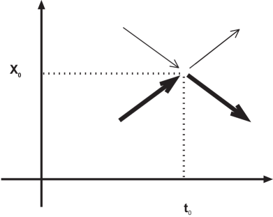
FIG. 2.: Furthest point of excursion

A few will overshoot a moment later to attain higher values $x>x_{0}$ that are far less probable, still others will have come from higher values. But the majority will turn around at $x_{0}$ to move back towards $x=0$.

The ensemble average will follow suit, to arrive at $x_{1}$ just slightly smaller than $x_{0}$. Here, the ensemble is considerably modified by re-establishing equilibrium, as further microstates, with $x_{1}$ as their excursion peak, join in. As the new members greatly outnumber the old ones, the ensemble average now follows these to move still closer to equilibrium. It is this ensemble-averaging at every step, over an ever increasing group of microstates representing ever more probable macrostates, that increases the entropy, forces the macrostate towards equilibrium and renders the macroscopic dynamics irreversible.

In the macroscopic formulation, $\dot{x}=-x/\tau$, this physics is accounted for by the dissipative term on the right side $\sim x$. Its form is valid irrespective of the underlying microscopic dynamics, which certainly does not contain any such term. In a sense, $x$ only measures the “entropic distance” to equilibrium.

The same is true for the heat diffusion equation (in a stationary medium), where the only current $\sim\nabla T$ is again entropic and does not reflect an underlying microscopic dynamics: The thermodynamic force $\nabla T$ vanishes in equilibrium, same as $x$, and is again a measure of the distance from it. So both types of macroscopic dynamics are in fact quite similar in their construction, with the only difference that the variable carrying out diffusion macroscopically is a conserved quantity. In the cases $\pi_{ij}+\pi^{D}_{ij}$, ${\bf H+H}^{D}$, ${\bf E+E}^{D}$, the respective first term does reflect the microscopic dynamics, while the second term is entropic. They measure the distance from equilibrium and nudge the respective field towards it.

Summarizing, we conclude that since ${\bf E}^{M}$ and ${\bf H}^{M}$ are not simply the spatial average of ${\bf e}$ and ${\bf h}$, there is no good reason to rule out the dissipative fields ${\bf E}^{D}$ and ${\bf H}^{D}$. A corollary result is the difference between the stationary solution, $\nabla\times\bf{E}^{M}$, $\nabla\times\bf{H}^{M}=0$, and the equilibrium configuration $\nabla\times\bf{E}$, $\nabla\times\bf{H}=0$. The same must hold in the linear response theory, but does not in its usual version, as we shall find out in the next section.

VII Linear Response Revisited

Let us recapitulate the usual derivation of the macroscopic Maxwell equations, due to Lorentz. Start from the microscopic Maxwell equations containing only ${\bf b}$ and ${\bf e}$, divide the charge into $\langle\varrho_{e}\rangle$, $\nabla\cdot{\bf p}$, the current into $\langle{\bf j_{e}}\rangle$, $\partial_{t}{\bf p}$, $\nabla\times{\bf m}$, and define ${\bf h}={\bf b}-{\bf m}$, ${\bf d}={\bf e}+{\bf p}$ to eliminate ${\bf p}$, ${\bf m}$ while preserving the structure of the original equations. These simple, identical algebraic manipulations already yield the structure of the macroscopic Maxwell equations, albeit in terms of ${\bf b},{\bf h},{\bf d},{\bf e}$. Therefore, these equations are still detailed, reversible, and completely equivalent to the starting point. A follow-up spatial averaging is easily executed, as the Maxwell equations are linear, and substitute $\langle{\bf b}\rangle,\langle{\bf h}\rangle,\langle{\bf d}\rangle,\langle{\bf e}\rangle$ for ${\bf b},{\bf h},{\bf d},{\bf e}$. Now these equations are of low resolution, yet they have retained the time reversal symmetry.

The next step, deceptively simple, is the crucial one. It introduces irreversibilities and takes us across the Rubicon into coarse-grained, macroscopic physics — although this step is usually considered the input of material properties, extrinsic to the Maxwell equations proper. We identify the variables, ${\bf B}\equiv\langle{\bf b}\rangle$, ${\bf D}\equiv\langle{\bf d}\rangle$, and (instead of going through the averaging over ever increasing ensembles) substitute $\langle{\bf h}\rangle,\langle{\bf e}\rangle$ with ${\bf H}^{M},{\bf E}^{M}$, and take the latter as functions of ${\bf B},{\bf D}$ and their temporal derivatives. Retaining only first order derivatives, we have

$${\bf E}^{M} = {\bf D}/\bar{\varepsilon}+(\beta/\varepsilon_{0})\dot{\bf D},$$ (18)

$${\bf H}^{M} = {\bf B}/\bar{\mu}+(\alpha/\mu_{0})\dot{\bf B},$$ (19)

or in Fourier space,

$${\bf D} = \bar{\varepsilon}{\bf E}^{M}/(1-i\omega\beta\bar{\varepsilon}/\varepsilon_{0}),$$ (20)

$${\bf B} = \bar{\mu}{\bf H}^{M}/(1-i\omega\alpha\bar{\mu}/\mu_{0}),$$ (21)

where $\bar{\varepsilon},\bar{\mu},\alpha,\beta$ are positive coefficients chosen to coincide with the hydrodynamic notation. Note especially the lack of time reversal symmetry of Eqs(18).

Two points here need amplification. First, it would not have been correct to take ${\bf D}$ as a function of ${\bf E}^{M}$ and its derivatives: Generally, starting from a temporally nonlocal relationship between ${\bf D}$ and ${\bf E}^{M}$, both seem possible, and one would need microscopic details to decide which is realized in a specific case. Furthermore, since the microscopic field $\bf d$ contains the polarization $\bf p$, it is considered an auxiliary field, and preferred by many to depend on the true field $\bf e$ — to lowest order in $\omega$ in the form

$${\bf D}=\bar{\varepsilon}({\bf E}^{M}-\beta\bar{\varepsilon}\dot{\bf E}^{M}/\varepsilon_{0}),$$ (22)

written such that $\varepsilon=D/E^{M}$ remains unchanged from Eq(20) in the given order. However, this formula is unacceptable on general grounds, irrespective of the microscopics. Assume homogeneity and stationarity in Eqs(13), $\nabla\times{\bf E}^{M}$, $\nabla\times{\bf H}^{M}$, $\dot{\bf D}$, $\dot{\bf B}=0$, and find Eq(22) producing a run-away solution $\dot{E}^{M}\sim\exp(t/\beta\bar{\varepsilon})$. (One must not change the minus sign in Eq(22) to render the solution decaying, as this would result in self-amplifying electromagnetic waves.)

The second point concerns the lack of spatial nonlocality, or why the permeabilities $\varepsilon$ and $\mu$ have not been taken as functions of the wave vector $q$. Usually, the answer entails a discussion of correlation lengths, which (for simplicity) takes place in an infinite medium. And the result is that spatial nonlocality becomes important only at microscopically small scales, so is usually negligible — except perhaps in systems with fast moving charge carriers, such as dilute plasmas. Let us, however, consult the hydrodynamic theory, the concept and considerations of which naturally include boundaries. It is in fact quite unambiguous on this point, and it must be completely equivalent to the linear response theory in the parameter space where both the frequency and the field strength are low, and where the two stripes, A and B of Fig 1, overlap. Assuming constant temperature, we may rewrite Eqs(15,16) as

$${\bf E}^{D}=(\beta/\varepsilon_{0}){\bf\dot{D}} +\lambda^{2}\nabla\times\nabla\times{\bf E},$$ (23)

$${\bf H}^{D}=(\alpha/\mu_{0}){\bf\dot{B}} +\lambda^{2}\nabla\times\nabla\times{\bf H},$$ (24)

where

$$\lambda=c\sqrt{\alpha\beta}.$$ (25)

If either $\alpha$ or $\beta$ is very small, the two terms $\sim\lambda^{2}$ may be neglected. Then these two equations – via Eqs(5) and (14) – reduce to the usual linear response expressions, Eqs(18,20). However, there are also cases in which $\lambda$ cannot be neglected: Being proportional to the relaxation time of magnetization and polarization, cf Eq(17), $\alpha$ and $\beta$ vary greatly, from $\beta\approx 10^{-15}$s for transparent dielectrics, to $\alpha\approx 10^{-5}$s for colloidal magnetic liquids (Rosensweig 1985, Shliomis 1974); while water (or any other matrix liquid with a strong, permanent molecular dipole moment) is in the middle range, $\beta\simeq 10^{-9}$s. So a water-based ferrofluid should have a colossal $\lambda\simeq 3\rm x10^{3}$cm.

There is a statement about dielectric media, found in every textbook on electromagnetism: If the electric and magnetic field are static, they are longitudinal and decoupled from each other. It is true if the usual linear response theory, Eqs(18,20), holds: Setting ${\bf\dot{D}}$, ${\bf\dot{B}}=0$, we have $\nabla\times{\bf E},\ \nabla\times{\bf H}=0$, and the only stationary solution are indeed longitudinal, decoupled and in equilibrium. But it is not true in the general case, as the more complete version of the linear response theory, Eqs(23,24), or simpler, the hydrodynamic theory, Eqs(13,14,16), entertains a stationary solution that is off-equilibrium and of the form

$$E_{x} = ({\cal E_{+}}e^{z/\lambda}+{\cal E_{-}}e^{-z/\lambda})/\sqrt{\varepsilon_{0}},$$ (26)

$$H_{y} = ({\cal E_{+}}e^{z/\lambda}-{\cal E_{-}}e^{-z/\lambda})\sqrt{\alpha/(\beta\mu_{0})},$$ (27)

where $\cal E_{\pm}$ are constant amplitudes. These electric and magnetic field are coupled and transverse, they start off from the boundary and relax exponentially into the bulk. Since the presence of a boundary makes itself felt over the distances of $\lambda$, a dielectric ferrofluid is indeed a dense and strongly interacting system that entertains a macroscopically large spatial nonlocality. It would be interesting to detect these fields, and fortunately, this does not appear to be difficult.

[Take a slab of dielectric ferrofluid, with a width $L\ll\lambda$, say 1cm. Expose this liquid to an oscillating electric or magnetic field, tangential to the slab, of the frequency $\omega\ll c/L$, and measure the internal field. Conventionally, we expect the result to be a uniform internal field, $E$ or $H$, that oscillates in phase with the external one and has the same magnitude, so $D$ and $B$ display a phase lag $\sim\varepsilon^{\prime\prime},\mu^{\prime\prime}$. The hydrodynamic consideration includes the stationary solution above, and the result depends on the type of the containing plates: If they are nonconducting, the phase lag has the same magnitude but an opposite sign; if they are conducting, the internal electric field should be drastically reduced (Liu 1997).]

VIII Electromagnetic Forces

Given the input of the thermodynamic theory, the basic form of the Maxwell equations and the relevant conservation laws, the derivation of the complete hydrodynamic theory is an exercise in cogent deduction and algebraic manipulation (Khalatnikov 1965, Henjes and Liu 1993). One of the main results is the expression for the total stress tensor, $\Pi_{ij}=\pi_{ij}+\pi^{D}_{ij}$: The first is the Lorentz-Galilean boosted Maxwell tensor, the second is the dissipative, off-equilibrium contribution, of the usual form and $\sim v_{ij}$ if the liquid is isotropic and the external field weak. [Otherwise, it will contain terms $\sim\nabla\times{\bf E}$, $\nabla\times{\bf H}$, cf Liu (1994).] Inserting the explicit expression for $\Pi_{ij}$ into Eq(8), and combining it with and Eqs(13), we obtain a transparent form of the momentum conservation,

$$\rho(\textstyle{\frac{\partial}{\partial t}}+v_{j}\nabla_{j})[v_{i}+({\bf E\times H}/c^{2}-{\bf D\times B})_{i}/\rho]$$ (28)

$$+s\nabla_{i}T+\rho_{1}\nabla_{i}\mu_{1}+\rho_{2}\nabla_{i}\mu_{2}+g_{j}\nabla_{i}v_{j}$$ (29)

$$=\left(\langle\rho^{e}\rangle{\bf E}+\langle{\bf j^{e}\rangle\times B}+{\bf f^{D}}\right)_{i}-\nabla_{j}\pi^{D}_{ij}.$$ (30)

The first line contains both the acceleration $\rho\mbox{\boldmath$\dot{v}$}$ and the Abraham-force $\frac{\partial}{\partial t}({\bf E\times H}/c^{2}-{\bf D\times B})$. (The latter is a small quantity if the electromagnetic wave length of a given frequency is large compared to the experimental dimension, as is usual for hydrodynamic frequencies.) The four terms of the next line are the proper generalization of the pressure gradient and include the reactive ponderomotive forces. They are valid for a two-component medium (such as a solution), with $\rho_{1}$, $\rho_{2}$ denoting the respective density, and $\rho=\rho_{1}+\rho_{2}$. Given linear constitutive relations, assuming that $\bar{\varepsilon}-\varepsilon_{0}$, $\bar{\mu}-\mu_{0}$ are proportional to one of the densities but independent of the other, and neglecting contributions $\sim{\cal O}(v/c)$, they reduce to the usual Kelvin force,

$\displaystyle\nabla P-\textstyle{\frac{1}{2}}(\bar{\varepsilon}-\varepsilon_{0})\nabla E^{2}-\textstyle{\frac{1}{2}}(\bar{\mu}-\mu_{0})\nabla H^{2},$

where $P$ is the pressure in the absence of fields. The third line, finally, contains the dissipative stress tensor $\pi^{D}_{ij}$, the Lorentz force — in terms of $E$ rather than $E^{M}$, in contrast to Eq(3) — and the novel dissipative ponderomotive force,

$${\bf f^{D}}={\bf B\times\nabla\times H^{D}+D\times\nabla\times E^{D}}.$$ (31)

It is odd under time reversal, same as $\pi^{D}_{ij}$, and accounts for forces that arise because the polarization and magnetization are not quite in equilibrium.

As we shall soon realize, terms in ${\bf f^{D}}$ of linear order in $v/c$ may be just as important as those of zeroth order. They have been neglected above to keep the arguments and display simple, but are easily retrieved: The fields in the Euler Eqs(7), and hence in the dissipative fields, are those of the local rest frame,

$${\bf H}^{D} = -(\alpha/\mu_{0})\nabla\times{\bf E^{0}},\quad{\bf E}^{D}=(\beta/\varepsilon_{0})\nabla\times{\bf H^{0}},$$ (32)

$${\bf E^{0}} = {\bf E}+\mbox{ \boldmath$v$}\times{\bf B},\quad{\bf H^{0}}={\bf H}-\mbox{\boldmath$v$}\times{\bf D}.$$ (33)

This is plausible: The question whether equilibrium is established in a system cannot depend on the observer’s choice of the inertial frame. [The derivation consists of generalizing the results of Eqs(6,7,16) to systems with finite velocities, where a pragmatic combination of Galilean and first order Lorentz transformation is employed. A fully covariant theory (Kostädt and Liu 1998) was also derived to make sure that the additional terms are indeed negligible in usual circumstances (Symalla and Liu 1998).]

Assuming for simplicity that $\beta$ (and hence $E^{D}$) is negligible, and confining our considerations to incompressible systems of simple geometry — a sphere or a slab such that the internal field are uniform — we may rewrite $H^{D}$ as

$${\bf H^{D}}=(\alpha/\mu_{0})[{\bf\dot{B}}-({\bf B}\cdot\nabla)\mbox{\boldmath$v$}],$$ (34)

where the second term, of order $v/c$, is a result of the fact that ${\bf H^{D}}$ is given in terms of the restframe field ${\bf E^{0}}$, rather than ${\bf E}$.

First, consider a solid magnetic sphere, $\mbox{\boldmath$v$}=\Omega\times\mbox{ \boldmath$r$}$, and expose it to a rotating magnetic field of the frequency $\Omega_{B}$. If there are no further perturbations, all forces except ${\bf f^{D}}$ vanish, and ${\bf H^{D}}=(\alpha/\mu_{0})[(\mbox{\boldmath$\Omega_{B}-\Omega$})\times{\bf B}]$. The torque on the sphere, after being partially integrated (over a surface slightly larger than the sphere), is $\int dV(\mbox{\boldmath$r$}\times{\bf f^{D}})=\int dV({\bf B\times H^{D}})$. With $\Theta$ denoting the sphere’s moment of inertia, Eq(8) therefore reduces to,

$$\mbox{\boldmath$\dot{\Omega}$}=(\alpha V/\Theta\varepsilon_{0})\ {\bf B}\times[(\mbox{\boldmath$\Omega_{B}-\Omega$})\times{\bf B}].$$ (35)

After an initial surprise, it is reassuring to see how these two terms of successive orders in $v/c$ cancel each other if the magnetic field and the sphere co-rotate – as they must to conserve total angular momentum. (A curiously similar effecr at linearly polarized magnetic field was observed by Gazeau et al, 1997)

Next, consider a slab of ferrofluid sustaining a shear flow $\nabla_{n}v_{t}$, where the subscripts denote the normal and tangential direction with respect to the slab. If $\dot{B}=0$, only the second term of Eq(34) remains, which represents a correction to the viscosity $\eta$,

$$\rho\dot{v}_{t}=\eta_{e}\nabla^{2}_{n}v_{t},\quad\eta_{e}=\eta+(\alpha/\mu_{0})B^{2}\cos^{2}\varphi,$$ (36)

where $\varphi$ denotes the angle between $B$ and the slab normal. [In the presence of a magnetic field, the viscosity $\eta$ itself is a function of $B$ and its orientation. Therefore, the information about this contribution of $\alpha$ is not easily extracted experimentally.]

If the field oscillates in time, the first term in Eq(34) becomes important, $\rho\dot{v}_{t}-\eta_{e}\nabla^{2}_{n}v_{t}=B_{n}\dot{B}_{t}\nabla_{n}\alpha/\mu_{0}$. Because $\alpha$ (as a function of temperature and density) is constant within the ferrofluid, the right side is nonvanishing only at the surface, where $\alpha$ jumps discontinuously to zero. So this force is best accounted for with boundary conditions. Solving $\rho\dot{v}_{t}=\eta_{e}\nabla^{2}_{n}v_{t}$, the boundary conditions are

$$\eta_{e}\nabla_{n}v_{t}=(\alpha/\mu_{0})B_{n}\dot{B}_{t},\qquad v_{t}=0,$$ (37)

for a free and sticking surface, respectively. [The free condition is obtained by setting the off-diagonal stress tensor $\Pi_{tn}$ to zero, while heeding the fact that $H^{M}_{t}$, rather than $H_{t}$, is continuous across the interface.]

Expose a slab of ferrofluid with its free surface facing upward to a static normal and an oscillating tangential field. If the frequency is low enough, we may neglect $\rho\dot{v}_{t}$, and the gradient given by Eq(37) is constant throughout the width $L$ of the slab. Since $v_{t}=0$ at the bottom, the averaged velocity is $\langle v_{t}\rangle=(\alpha/\mu_{0})B_{n}\dot{B}_{t}L/2\eta_{e}$.

Now forget the gravity, bend this slab into a ring with the free surface facing inward, and expose this construct to a $B$-field rotating in the plane of the ring. Take the momentary orientation of the field as $\hat{x}$, then a counter-clockwise rotation has $\dot{B}$ along $\hat{y}$. In the two sections of the ring perpendicular to $\hat{x}$, the gradient of the velocity, according to Eq(37), is positive. Because the velocity must vanish at the outer rim of the two sections, it is negative in the right section, and positive in the left. They combine to yield a clockwise circular flow, opposite to the external field.

In an open, round vessel, the free surface of the ferrofluid (facing upward) curves up at the wall, as wetting fluids do. And the capillary region is very similar to such a sheet of circular flow, and should rotate opposite to the external field — while the bulk of the fluid below rotates, more or less, with this region (Rosensweig et al 1990).

All these effects follow cogently from the identification of $\nabla\times{\bf E^{0}}$ as the magnetic thermodynamic force. They depend on only one parameter $\alpha$ that has a clear-cut physical significance and a definite value. In addition, there is a one-to-one correspondence to the analogous effects stemming from the dissipative, ponderomotive electric force, ${\bf D\times\nabla\times E^{D}}$.