Fisher zeros of the $Q$-state Potts model in the complex temperature plane for nonzero external magnetic field

Abstract

The microcanonical transfer matrix is used to study the distribution of the Fisher zeros of the $Q>2$ Potts models in the complex temperature plane with nonzero external magnetic field $H_{q}$. Unlike the Ising model for $H_{q}\neq 0$ which has only a non-physical critical point (the Fisher edge singularity), the $Q>2$ Potts models have physical critical points for $H_{q}<0$ as well as the Fisher edge singularities for $H_{q}>0$. For $H_{q}<0$ the cross-over of the Fisher zeros of the $Q$-state Potts model into those of the ($Q-1$)-state Potts model is discussed, and the critical line of the three-state Potts ferromagnet is determined. For $H_{q}>0$ we investigate the edge singularity for finite lattices and compare our results with high-field, low-temperature series expansion of Enting. For $3\leq Q\leq 6$ we find that the specific heat, magnetization, susceptibility, and the density of zeros diverge at the Fisher edge singularity with exponents $\alpha_{e}$, $\beta_{e}$, and $\gamma_{e}$ which satisfy the scaling law $\alpha_{e}+2\beta_{e}+\gamma_{e}=2$.

I introduction

The $Q$-state Potts model[1, 2] in two dimensions exhibits a rich variety of critical behavior and is very fertile ground for the analytical and numerical investigation of first- and second-order phase transitions. With the exception of the $Q=2$ Potts (Ising) model in the absence of an external magnetic field[3], exact solutions for arbitrary $Q$ are not known. However, some exact results have been established for the $Q$-state Potts model. For $Q=2$, 3 and 4 there is a second-order phase transition, while for $Q>4$ the transition is first order[4]. From the duality relation the critical temperature is known to be $T_{c}=J/k_{B}{\rm ln}(1+\sqrt{Q})$[1]. For $Q=3$ and 4 the critical exponents[5] are known, while for $Q>4$ the latent heat[4], spontaneous magnetization[6], and correlation length[7] at $T_{c}$ are also known.

By introducing the concept of the zeros of the partition function in the complex magnetic-field plane (Yang-Lee zeros), Yang and Lee[8] proposed a mechanism for the occurrence of phase transitions in the thermodynamic limit and yielded a new insight into the unsolved problem of the Ising model in an arbitrary nonzero external magnetic field. Lee and Yang[8] also formulated the celebrated circle theorem which states that the Yang-Lee zeros of the Ising ferromagnet lie on the unit circle $x_{0}=e^{i\theta}$ in the complex $x={\rm exp}(\beta H)$ plane for any size lattice and any type of boundary conditions. The density of zeros contains all the information about a system and in particular in the thermodynamic limit the density of zeros completely determine the critical behavior of the system[8, 9, 29]. For example, the spontaneous magnetization of the Ising model is determined by the density of zeros on the positive real axis, i.e., $m_{0}(T)=2\pi g(\theta=0,T)$. Above the critical temperature $T_{c}$, there is a gap in the distribution of zeros, centered at $\theta=0$, that is, $g(\theta,T)=0$ for $|\theta|<\theta_{0}(T)$. Within this gap the free energy is analytic and there is no phase transition. The Yang-Lee zeros at $\theta=\pm\theta_{0}$ are called the Yang-Lee edge zeros. As $T-T_{c}\to 0^{+}$, $\theta_{0}(T)\to 0$. At $T_{c}$ the gap disappears, i.e., $\theta_{0}(T_{c})=0$, and $g(0,T_{c})=0$, which is the characteristic of a second-order phase transition. Below $T_{c}$, $g(0,T)>0$ and we have a finite spontaneous magnetization. Kortman and Griffiths[10] carried out the first systematic investigation of $g(\theta,T)$, based on the high-field, high-temperature series expansion for the Ising model on the square lattice and the diamond lattice. They found that above $T_{c}$, $g(\theta,T)$ diverges at $\theta=\pm\theta_{0}$, i.e., at the Yang-Lee edge singularity for the square lattice. The divergence of the density of the Yang-Lee zeros means the magentization diverges, which does not occur at a physical critical point. Fisher[11] proposed the idea that the singularity at the Yang-Lee edge can be thought of as a new second-order phase transition with associated critical exponents and the Yang-Lee edge zero can be considered as a conventional critical point. Fisher also renamed the Yang-Lee edge zero as the Yang-Lee edge singularity. The critical point of the Yang-Lee edge singularity is associated with a $\phi^{3}$ theory, different from the usual critical point associated with the $\phi^{4}$ theory. The crossover dimension of the Yang-Lee edge singularity is $d_{c}=6$. The study of the Yang-Lee edge singularity has been extended to the classical $n$-vector model[12], the quantum Heisenberg model[12], the spherical model[13], the quantum one-dimensional transverse Ising model[14], the hierarchical model[15], and the one-dimensional Potts model[16]. Using Fisher’s idea and conformal field theory, Cardy [17] studied the Yang-Lee edge singularity for a two-dimensional $\phi^{3}$ theory. Recently the Yang-Lee zeros of the two-dimensional $Q$-state Potts model have been studied[31].

In 1964 Fisher[18] emphasized that the partition function zeros in the complex temperature plane (Fisher zeros) is also very useful in understanding phase transitions. In particular, in the complex temperature plane both the ferromagnetic phase and the antiferromagnetic phase can be considered at the same time. From the exact solutions[3] of the square lattice Ising model Fisher conjectured that in the absence of an external magnetic field the zeros of the partition function lie on two circles in the complex $y={\rm exp}(-\beta J)$ plane given by $y_{FM}=-1+\sqrt{2}e^{i\theta}$ (ferromagnetic circle) and $y_{AFM}=1+\sqrt{2}e^{i\theta}$ (antiferromagnetic circle). Fisher also showed that the logarithmically infinite specific heat singularity of the Ising model results from the properties of the density of zeros. By numerical investigations[19] and analytical methods[20] it has been concluded that for very special boundary conditions the Fisher zeros of the Ising model do indeed lie on two circles, while for more general boundary conditions the zeros approach two circles as the size of lattices increases. Recently the locus of the Fisher zeros of the $Q$-state Potts model in the absence of an external magnetic field has been studied extensively[21, 22, 23, 25, 30]. It has been shown[23] that for self-dual boundary conditions near the ferromagnetic critical point $y_{c}=1/(1+\sqrt{Q})$ the Fisher zeros of the Potts model on a finite square lattice lie on the circle with center $-1/(Q-1)$ and radius $\sqrt{Q}/(Q-1)$ in the complex $y$-plane, while the antiferromagnetic circle of the Ising model completely disappears for $Q>2$. It is also known[23] that all the Fisher zeros of the one-state Potts model lie at $y^{-1}=0$. Shrock et al. showed that for the two-dimensional Ising[24] and Potts[25] models in the absence of an external magnetic field there exist non-physical critical points in the complex temperature plane, at which thermodynamic functions including the magnetization diverge. Itzykson et al.[26] considered the Fisher zeros in an external magnetic field for the first time. They studied the movement of the Fisher zero closest to the positive real axis for the Ising model as the strength of a magnetic field changes. For nonzero magnetic field there is a gap in the distribution of the Fisher zeros of the Ising model around the positive real axis even in the thermodynamic limit, which means that there is no phase transition. Matveev and Shrock[27] studied the Fisher zeros of the two-dimensional Ising model in an external magnetic field using the high-field, low-temperature series expansion and the partition functions of finite-size systems. They found that for nonzero magnetic field the magnetization, susceptibility, specific heat, and the density of zeros diverge at the Fisher zero closest to the positive real axis, which we call the Fisher edge singularity. In this paper we discuss the Fisher zeros of the $Q$-state Potts model for nonzero magnetic field using the microcanonical transfer matrix and the high-field, low-temperature series expansion.

II microcanonical transfer matrix and symmetries

The $Q$-state Potts model on a lattice $G$ in an external magnetic field $H_{q}$ is defined by the Hamiltonian

$${\cal H}_{Q}=-J\sum_{<i,j>}\delta(\sigma_{i},\sigma_{j})-H_{q}\sum_{k}\delta(\sigma_{k},q),$$ (1)

where $J$ is the coupling constant, $<i,j>$ indicates a sum over nearest-neighbor pairs, $\sigma_{i}=0,...,Q-1$, and $q$ is a fixed integer between 0 and $Q-1$. The partition function of the model is

$$Z_{Q}=\sum_{\{\sigma_{n}\}}e^{-\beta{\cal H}_{Q}},$$ (2)

where $\{\sigma_{n}\}$ denotes a sum over all possible configurations and $\beta=(k_{B}T)^{-1}$. The partition function can be written as

$$Z_{Q}=y^{-N_{b}}\sum_{E=0}^{N_{b}}\sum_{M=0}^{N_{s}}\Omega_{Q}(E,M)x^{M}y^{E},$$ (3)

where $x=e^{\beta H_{q}}$, $y=e^{-\beta J}$, $E$ and $M$ are positive integers $0\leq E\leq N_{b}$ and $0\leq M\leq N_{s}$, respectively, $N_{b}$ and $N_{s}$ are the number of bonds and the number of sites on the lattice $G$, and $\Omega_{Q}(E,M)$ is the number of states with fixed $E$ and fixed $M$. Using the microcanonical transfer matrix ($\mu$TM) [28, 29, 30, 31] we have calculated the number of states $\Omega_{Q}(E,M)$ of the $Q$-state Potts model on finite square lattices with self-dual boundary conditions[23] and cylindrical boundary conditions for $3\leq Q\leq 8$.

In the absence of an external magnetic field the partition function of the $Q$-state Potts model is symmetric under the dual transformation

$$y\to{1-y\over 1+(Q-1)y},$$ (4)

which gives the critical point

$$y_{c}={1\over 1+\sqrt{Q}}$$ (5)

and the invariant ferromagnetic circle of the Fisher zeros

$$y_{0}(\theta)={-1+\sqrt{Q}e^{i\theta}\over Q-1}.$$ (6)

The partition function of the Ising model has the additional symmetry

$$y\to{1\over y},$$ (7)

which maps the ferromagnetic Ising model to the antiferromagnetic model. This, together with the dual transformation, implies the invariance of the antiferromagnetic circle

$$y_{0}=1+\sqrt{2}e^{i\theta}.$$ (8)

However, the $Q>2$ Potts models do not possess this second symmetry and the associated Fisher zeros are scattered in the non-critical region. For nonzero magnetic field the Ising model also has the symmetry

$$x\to{1\over x},$$ (9)

and the Fisher zeros for $0<x<1$ have the same properties as those for $1<x<\infty$. The $Q>2$ Potts models do not have this symmetry, and distribution of zeros for $0<x<1$ is different from the distribution for $1<x<\infty$. Because the $Q>2$ Potts models are less symmetric than the Ising model, the zeros of the partition function have a much richer structure. For example, the Ising model has only non-physical critical points in the complex $y$-plane for $x\neq 1$, while the $Q>2$ Potts models have both non-physical and physical critical points in the same plane for $x\neq 1$. In this paper we study the Fisher zeros of the $Q$-state Potts model for nonzero magnetic field to unveil some of the rich structures of the model.

III Fisher zeros of the three-state Potts model for $x<1$

In the limit $H_{q}\to-\infty$ ($x\to 0$) the partition function of the $Q$-state Potts model becomes

$$Z_{Q}=y^{-N_{b}}\sum_{E=0}^{N_{b}}\Omega_{Q}(E,M=0)y^{E},$$ (10)

where $\Omega_{Q}(E,M=0)$ is the same as the number of states $\Omega_{Q-1}(E)$ of the ($Q-1$)-state Potts model in the absence of an external magnetic field. As $x$ decreases from 1 to 0, the $Q$-state Potts model is transformed into the ($Q-1$)-state Potts model in zero external field. Figure 1 shows the Fisher zeros in the complex $y$-plane of the three-state Potts model for $x\leq 1$ with self-dual boundary conditions. Note that in the absence of an external magnetic field for self-dual boundary conditions the Fisher zeros in the critical region of the Potts model lie on the circle given by Eq. (6)[23]. In Figure 1 (a) the circle is that of Eq. (6) with $Q=3$ (the three-state Potts circle), while in Figures 1 (c) and 1 (d) the circle is for $Q=2$ (the Ising circle). In Figure 1 (b) we show both the the three-state Potts circle (smaller one) and the Ising circle (larger one), and the Fisher zeros lie on neither the three-state Potts circle nor the Ising circle. In Figure 1 (c) the Fisher zeros near the ferromagnetic critical point begin to approach the Ising circle, and the antiferromagnetic circle of the Ising model begins to appear. In Figure 1 (d) almost all of the Fisher zeros, which will ultimately lie on the ferromagnetic circle of the Ising model at $x=0$, are very close to this locus, and the antiferromagnetic circle becomes clearer.

IV critical point of the three-state Potts model in a field $H_{q}<0$

For an external field $H_{q}<0$, one of the Potts states is supressed relative to the others. The symmetry of the Hamiltonian is that of the $(Q-1)$-state Potts model in zero external field, so that we expect to see cross-over from the $Q$-state critical point to the $(Q-1)$-state critical point as $-H_{q}$ is increased.

We have studied the field dependence of the critical point for $0\leq x\leq 1$ through the Fisher zero closest to the real axis, $y_{1}(x,L)$. For a given applied field $y_{1}$ approaches the critical point $y_{1}(L)\to y_{c}(x)$ in the limit $L\to\infty$, and the thermal exponent $y_{t}(L)$ defined as[22, 26]

$$y_{t}(L)=-{{\rm ln\{Im}[y_{1}(L+1)]/{\rm Im}[y_{1}(L)]\}\over{\rm ln}[(L+1)/L]}$$ (11)

will approach the critical exponent $y_{t}(x)$. Table I shows values for $y_{c}(x)$ extrapolated from calculations of $y_{1}(x,L)$ on $L\times L$ lattices for $3\leq L\leq 8$ using the Bulirsch-Stoer (BST) algorithm[32]. The error estimates are twice the difference between the ($n-1$,1) and ($n-1$,2) approximants[32]. The critical points for $x=1$ (three-state) and $x=0$ (two-state) Potts models are known exactly and are included in Table I for comparison. Note that the imaginary parts of $y_{c}$(BST) are all consistent with zero. We have also calculated the thermal exponent, $y_{t}$, applying the BST algorithm to the values given by Eq. (11), and these results are also presented in Table I. For $x=1$ we find $y_{t}$ very close to the known value $y_{t}=6/5$ for the three-state model, but for $x$ as large as 0.5 we obtain $y_{t}=1$, the value of the thermal exponent for the two-state (Ising) model.

Figure 2 shows the critical line of the three-state Potts ferromagnet for $H_{q}<0$. In Figure 2 the upper line is the critical temperature of the two-state model, $T_{c}(Q=2)=1/{\rm ln}(1+\sqrt{2})$, and the lower line is the critical temperature for the three-state model, $T_{c}(Q=3)=1/{\rm ln}(1+\sqrt{3})$. The critical line for small $-H_{q}$ is given by[33]

$$T-T_{c}(Q=3)\sim(-H_{q})^{y_{t}/y_{h}},$$ (12)

where $y_{t}=6/5$ and $y_{h}=28/15$ for the three-state Potts model.

V Fisher zeros of the three-state Potts model for $x>1$

In the limit $H_{q}\to\infty$ ($x\to\infty$) the positive field $H_{q}$ favors the state $q$ for every site and the $Q$-state Potts model is transformed into the one-state model[23]. The zeros are given by

$$Z_{Q}\sim y^{-N_{b}}\sum_{E=0}^{N_{b}}\Omega_{Q}(E,M=N_{s})y^{E}=0.$$ (13)

Because $\Omega_{Q}(E,M=N_{s})=1$ for $E=0$ and 0 otherwise, Eq. (13) is

$$y^{-N_{b}}=0.$$ (14)

As $x$ increases $|y_{0}|$ for all the zeros increases without bound.

Figure 3 shows the Fisher zeros in the complex $y$-plane of the three-state Potts model for $h=\beta H$ varying from 0 to 4 in steps of 1. As $h$ increases, all the Fisher zeros move away from the origin. Note that for $h>0$ there is accumulation of the Fisher zeros as we approach the Fisher edge zero, that is, the Fisher zero closest to the positive real axis. That kind of accumulation suggests that for $h>0$ the density of zeros diverges at the Fisher edge zero, which we call the Fisher edge singularity. The critical exponents associated with the edge singularity are defined in the usual way,

$$C_{e}\sim(1-{y\over y_{e}})^{-\alpha_{e}},$$ (15)

$$m_{e}\sim(1-{y\over y_{e}})^{\beta_{e}},$$ (16)

and

$$\chi_{e}\sim(1-{y\over y_{e}})^{-\gamma_{e}},$$ (17)

where $y_{e}$ is the location of the Fisher edge singularity, and $C_{e}$, $m_{e}$ and $\chi_{e}$ are the singular parts of the specific heat, magnetization, and susceptibility, respectively.

To study the critical behavior at the Fisher edge singularity we have used the high-field, low-temperature series expansion for the three-state Potts model due to Enting[34, 36], which is coded as partial generating functions. Table II shows estimates for $y_{e}$ and $\beta_{e}$ from Dlog Padé approximants[35] for the magnetization at $x=100$. For this value of $x$ we find $\alpha_{e}=1.22(2)$, $\beta_{e}=-0.197(6)$, and $\gamma_{e}=1.20(3)$. Note that both $\beta_{e}$ and $\alpha_{e}$ are unphysical in that $\beta_{e}<0$ implies a divergent magnetization and $\alpha_{e}>1$ implies a divergent energy density. The density of zeros near the Fisher edge singularity in the complex temperature plane is given by[18]

$$g(y)\sim(1-{y\over y_{e}})^{1-\alpha_{e}}.$$ (18)

Therefore, $\alpha_{e}>1$ means that the density of zeros diverges at the Fisher edge singularity. From $\alpha_{e}$, $\beta_{e}$, and $\gamma_{e}$ we obtain

$$\alpha_{e}+2\beta_{e}+\gamma_{e}=2.03(4),$$ (19)

so that the Rushbrooke scaling law $\alpha+2\beta+\gamma=2$, which is known to hold at a physical critical point, is also satisfied at the Fisher edge singularity. From the series expansions for the specific heat, magnetization, and susceptibility we have obtained the location of the Fisher edge singularity

$$y_{e}({\rm series})=1.232(2)+1.048(3)i,$$ (20)

which is in excellent agreement with the value we calculate by extrapolation from finite-size systems using the BST algorithm,

$$y_{e}({\rm BST})=1.233(7)+1.050(3)i.$$ (21)

We have also studied the critical behavior at the Fisher edge singularity for several values of $x$. Table III shows the edge critical exponents and the location of the Fisher edge singularity for $x=20$, 100 and 200. The edge critical exponents for any $x$ satisfy the relation $\alpha_{e}+2\beta_{e}+\gamma_{e}=2$ within our error estimates. The locations of the Fisher edge singularity obtained from the series analysis agree very well with those extrapolated from finite size data by the BST algorithm. Table III suggests that the values of the edge critical exponents are independent of $x$.

VI Fisher zeros of the $Q>3$ Potts models for nonzero magnetic field

Using the high-field, low-temperature series expansion of the $Q$-state Potts model for $4\leq Q\leq 6$[36], we have studied the critical behavior at the Fisher edge singularity for $Q>3$. Table IV shows the edge critical exponents and the locations of the Fisher edge singularities for $4\leq Q\leq 6$ and $x=100$. The edge critical exponents for any $Q$ satisfy the relation $\alpha_{e}+2\beta_{e}+\gamma_{e}=2$ within our error estimates. As $Q$ increases $\beta_{e}$ appears to decrease slightly, while $\alpha_{e}$ and $\gamma_{e}$ are constant within error. However, because the uncertainties in $\alpha_{e}$ and $\gamma_{e}$ are large, we do not know whether $\alpha_{e}$ and $\gamma_{e}$ are truly independent of $Q$. Even though the Yang-Lee edge singularities have never been studied for the two-dimensional $Q>2$ Potts models, according to the study of other models[10, 11, 12, 14] and conformal field theory[17] one expects the critical behavior of the Yang-Lee edge singularities in two dimensions to be universal. However, in a study[25] of the Fisher (or complex-temperature) singularities of the Potts model in the absence of an external magnetic field Shrock et al. have observed a dependence of the edge critical exponents on $Q$. In Table IV the BST estimates and the series results for the location of the Fisher edge singularities agree with each other for $Q=4$ and 5. For $Q=6$ we have calculated $\Omega_{Q}(E,M)$ up to $L=5$, and the BST extrapolation is unreliable because the maximum size of the lattice is small. Figure 4 shows the Fisher zeros in the complex $y$-plane of the six-state Potts model for $x=100$, and the location of the edge singularities calculated from the series, which has been the traditional method[25, 27] in the study of the Fisher (or complex-temperature) singularities.

VII conclusion

We have studied the Fisher zeros in the complex $y$-plane of the $Q$-state Potts model for $x\neq 1$ using the microcanonical transfer matrix and the high-field, low-temperature series expansion. We have discussed the transformation of the Fisher zeros of the $Q$-state Potts model into those of the ($Q-1$)-state Potts model for $x<1$, and into those of the one-state Potts model for $x>1$. For $x<1$ we have obtained the critical line and calculated the critical exponents for several values of $x$. From the high-field, low temperature series expansion we have shown that for $3\leq Q\leq 6$ the specific heat, magnetization, susceptibility, and the density of zeros diverge algebraically at the Fisher edge singularity with characteristic edge exponents $\alpha_{e}$, $\beta_{e}$, and $\gamma_{e}$.

TABLE I.: The critical temperature $y_{c}$ and the critical exponent $y_{t}$ of the three-state Potts model for $0\leq x\leq 1$.

$x$	$y_{c}$ (BST)	$y_{c}$ (exact)	$y_{t}$ (BST)	$y_{t}$ (exact)
0	$0.414(3)+0.0002(4)i$	0.414213…	1.001(2)	1
0.001	$0.414(3)+0.0002(4)i$		1.001(2)
0.05	$0.413(5)+0.0002(3)i$		1.0009(6)
0.5	$0.400(2)+0.000(2)i$		0.982(21)
1	$0.366(2)+0.0002(5)i$	0.366025…	1.195(3)	$6\over 5$

TABLE II.: Values of $\beta_{e}$ and $y_{e}$ estimated from Dlog Padé approximants to magnetization for $Q=3$ and $x=100$.

$[N/D]$	$\beta_{e}$	$y_{e}$
$[7/8]$	$-0.2077$	$1.243256+1.052564i$
$[8/8]$	$-0.1967$	$1.236604+1.045093i$
$[9/8]$	$-0.1952$	$1.237445+1.043712i$
$[8/9]$	$-0.1954$	$1.238006+1.043638i$
$[9/9]$	$-0.1957$	$1.236733+1.044346i$
$[10/9]$	$-0.1939$	$1.235093+1.044025i$
$[9/10]$	$-0.1956$	$1.235556+1.044725i$
$[10/10]$	$-0.1953$	$1.235416+1.044633i$
$[11/10]$	$-0.1930$	$1.233087+1.045059i$
$[10/11]$	$-0.1956$	$1.235523+1.044727i$
$[11/11]$	$-0.2003$	$1.233911+1.047358i$
$[12/11]$	$-0.1975$	$1.233556+1.046650i$
$[11/12]$	$-0.1972$	$1.233675+1.046438i$
$[12/12]$	$-0.1977$	$1.233538+1.046729i$
$[13/12]$	$-0.1975$	$1.233549+1.046638i$
$[12/13]$	$-0.1959$	$1.233478+1.046087i$
$[13/13]$	$-0.1991$	$1.233249+1.047366i$
$[14/13]$	$-0.1966$	$1.233340+1.046474i$
$[13/14]$	$-0.1943$	$1.232810+1.046075i$
$[14/14]$	$-0.1937$	$1.231850+1.046918i$
$[15/14]$	$-0.1970$	$1.233458+1.046527i$
$[14/15]$	$-0.1945$	$1.232889+1.046035i$
$[15/15]$	$-0.1945$	$1.231888+1.047107i$
$[16/15]$	$-0.1966$	$1.233328+1.046471i$

TABLE III.: The location and the edge critical exponents of the Fisher edge singularity for the three-state Potts model.

$x$	$y_{e}$ (BST)	$y_{e}$ (series)	$\alpha_{e}$	$\beta_{e}$	$\gamma_{e}$
20	$0.880(2)+0.643(2)i$	$0.880(4)+0.641(3)i$	1.2(1)	$-0.19(1)$	1.2(1)
100	$1.233(7)+1.050(3)i$	$1.232(2)+1.048(3)i$	1.22(2)	$-0.197(6)$	1.20(3)
200	$1.436(8)+1.270(1)i$	$1.436(2)+1.268(2)i$	1.22(2)	$-0.196(7)$	1.21(3)

TABLE IV.: The location and the edge critical exponents of the Fisher edge singularity for the $4\leq Q\leq 6$ Potts models and $x=100$.

$Q$	$y_{e}$ (BST)	$y_{e}$ (series)	$\alpha_{e}$	$\beta_{e}$	$\gamma_{e}$
4	$1.13(6)+0.96(4)i$	$1.159(5)+0.93(1)i$	1.18(8)	$-0.180(4)$	1.12(8)
5	$1.09(4)+0.861(8)i$	$1.103(4)+0.86(1)i$	1.2(1)	$-0.173(4)$	1.1(1)
6		$1.053(8)+0.811(4)i$	1.2(1)	$-0.164(9)$	1.1(1)

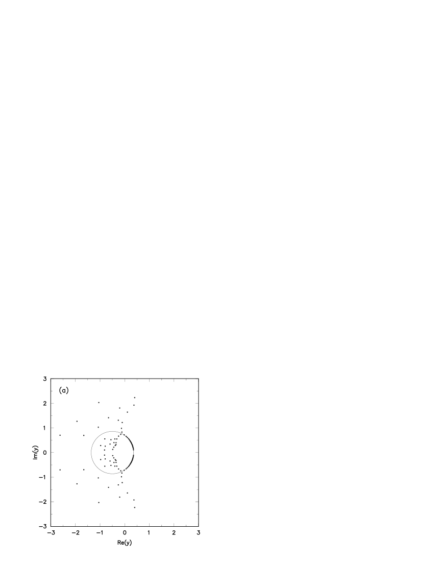
FIG. 1.: Fisher zeros in the complex $y$-plane of a $7\times 7$ three-state Potts model for (a) $x=1$, (b) 0.5, (c) 0.05, and (d) 0.001 with self-dual boundary conditions.

FIG. 2.: Critical temperatures of the three-state Potts ferromagnet as a function of the magnetic field. $H_{q}$ is in unit of $J$ and $T$ is in unit of $J/k_{B}$. The upper dotted line is the Ising transition temperature in the limit $H_{q}\to-\infty$, while the lower dotted line shows the critical temperature of the three-state Potts model for $H_{q}=0$.

FIG. 3.: Fisher zeros in the complex $y$-plane of an $8\times 8$ three-state Potts model for $h=\beta H$ varying from 0 to 4 in steps of 1 with cylindrical boundary conditions.

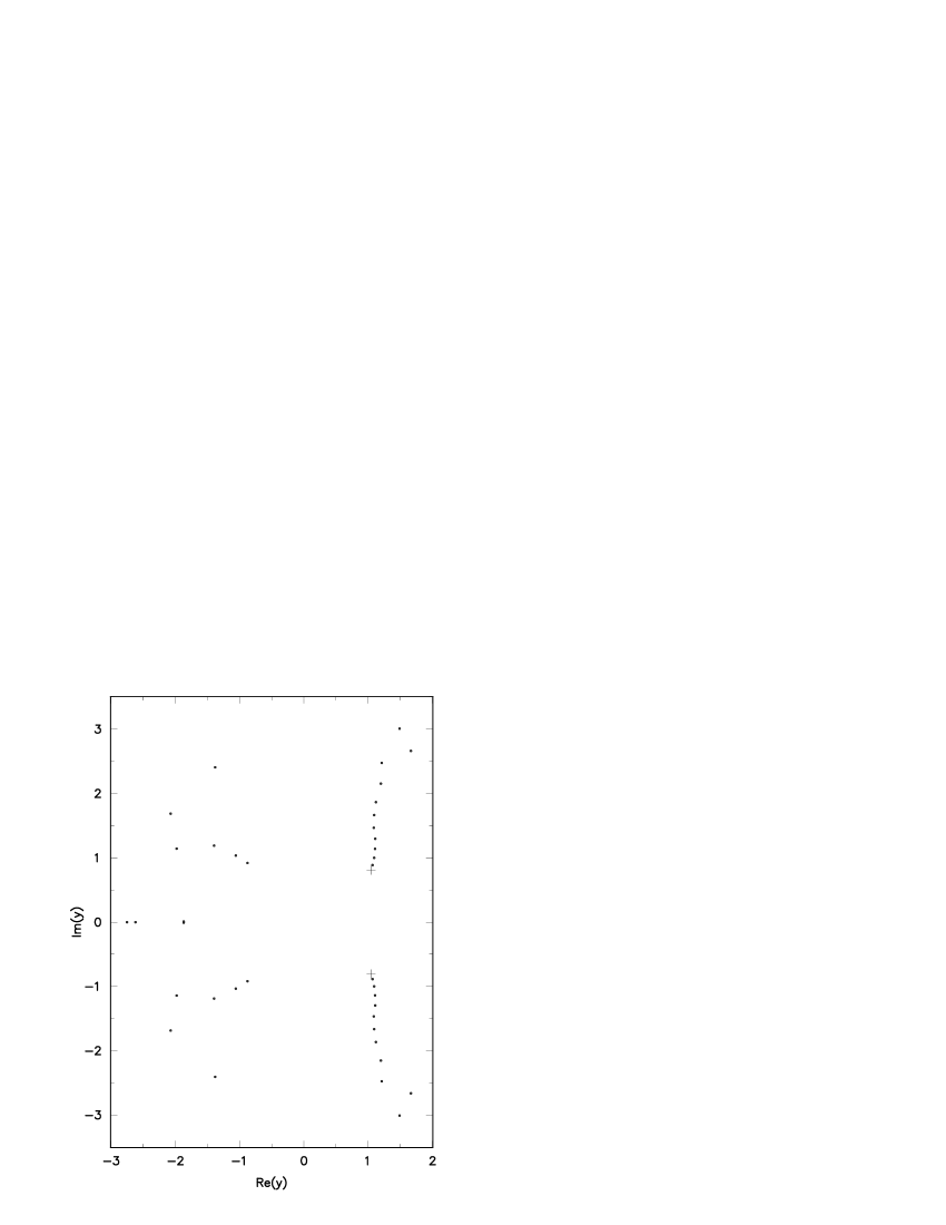
FIG. 4.: Fisher zeros in the complex $y$-plane of a $5\times 5$ six-state Potts model for $x=100$ with cylindrical boundary conditions. The two plus symbols show the locations of the Fisher edge singularities estimated from the series analysis.

REFERENCES

- [1] R. B. Potts, Proc. Cambridge Philos. Soc. 48, 106 (1952).
- [2] F. Y. Wu, Rev. Mod. Phys. 54, 235 (1982).
- [3] L. Onsager, Phys. Rev. 65, 117 (1944); B. Kaufman, ibid. 76, 1232 (1949).
- [4] R. J. Baxter, J. Phys. C 6, L445 (1973).
- [5] M. P. M. den Nijs, J. Phys. A 12, 1857 (1979); B. Nienhuis, E. K. Riedel, and M. Schick, ibid. 13, L189 (1980); R. B. Pearson, Phys. Rev. B 22, 2579 (1980); J. Black and V. J. Emery, ibid. 23, 429 (1981); M. P. M. den Nijs, ibid. 27, 1674 (1983); R. J. Creswick and S.-Y. Kim, J. Phys. A 30, 8785 (1997).
- [6] R. J. Baxter, J. Phys. A 15, 3329 (1982).
- [7] E. Buffernoir and S. Wallon, J. Phys. A 26, 3045 (1993).
- [8] C. N. Yang and T. D. Lee, Phys. Rev. 87, 404 (1952); T. D. Lee and C. N. Yang, ibid., 410 (1952).
- [9] R. Abe, Prog. Theor. Phys. 37, 1070 (1967); ibid. 38, 72 (1967); M. Suzuki, ibid., 1225 (1967); ibid., 1243 (1967); R. Kenna and C. B. Lang, Phys. Rev. E 49, 5012 (1994).
- [10] P. J. Kortman and R. B. Griffiths, Phys. Rev. Lett. 27, 1439 (1971).
- [11] M. E. Fisher, Phys. Rev. Lett. 40, 1610 (1978).
- [12] D. A. Kurtze and M. E. Fisher, Phys. Rev. B 20, 2785 (1979).
- [13] D. A. Kurtze and M. E. Fisher, J. Stat. Phys. 19, 205 (1978).
- [14] K. Uzelac, P. Pfeuty, and R. Jullien, Phys. Rev. Lett. 43, 805 (1979).
- [15] G. A. Baker, Jr., M. E. Fisher, and P. Moussa, Phys. Rev. Lett. 42, 615 (1979).
- [16] L. Mittag and M. J. Stephen, J. Stat. Phys. 35, 303 (1984); Z. Glumac and K. Uzelac, J. Phys. A 27, 7709 (1994).
- [17] J. L. Cardy, Phys. Rev. Lett. 54, 1354 (1985).
- [18] M. E. Fisher, in Lectures in Theoretical Physics, edited by W. E. Brittin (University of Colorado Press, Boulder, 1965), Vol. 7c, p. 1.
- [19] S. Katsura, Prog. Theor. Phys. 38, 1415 (1967); Y. Abe and S. Katsura, ibid. 43, 1402 (1970).
- [20] H. J. Brascamp and H. Kunz, J. Math. Phys. 15, 65 (1974).
- [21] P. P. Martin, Nucl. Phys. B 225, 497 (1983); J. M. Maillard and R. Rammal, J. Phys. A 16, 353 (1983); P. P. Martin and R. Rammal, ibid. 19, L547 (1986); D. W. Wood, R. W. Turnbull, and J. K. Ball, ibid. 20, 3465 (1987); J. C. A. d’Auriac, J. M. Maillard, G. Rollet, and F. Y. Wu, Physica A 206, 441 (1994).
- [22] G. Bhanot, J. Stat. Phys. 60, 55 (1990); N. A. Alves, B. A. Berg, and R. Villanova, Phys. Rev. B 43, 5846 (1991).
- [23] P. P. Martin, in Integrable Systems in Statistical Mechanics, edited by G. M. D’Ariano, A. Montorsi, and M. G. Rasetti (World Scientific, Singapore, 1985), p. 129; P. P. Martin, J. Phys. A 19, 3267 (1986); P. P. Martin, Potts Models and Related Problems in Statistical Mechanics (World Scientific, Singapore, 1991); C.-N. Chen, C.-K. Hu, and F. Y. Wu, Phys. Rev. Lett. 76, 169 (1996); F. Y. Wu, G. Rollet, H. Y. Huang, J. M. Maillard, C.-K. Hu, and C.-N. Chen, ibid., 173 (1996); R. Kenna, Nucl. Phys. B (Proc. Suppl.) 63, 646 (1998).
- [24] V. Matveev and R. Shrock, J. Phys. A 28, 1557 (1995); ibid. 29, 803 (1996).
- [25] V. Matveev and R. Shrock, Phys. Rev. E 54, 6174 (1996); H. Feldmann, R. Shrock, and S.-H. Tsai, ibid. 57, 1335 (1998); H. Feldmann, A. J. Guttmann, I. Jensen, R. Shrock, and S.-H. Tsai, J. Phys. A 31, 2287 (1998).
- [26] C. Itzykson, R. B. Pearson, and J. B. Zuber, Nucl. Phys. B 220, 415 (1983).
- [27] V. Matveev and R. Shrock, J. Phys. A 28, 4859 (1995); Phys. Rev. E 53, 254 (1996).
- [28] B. Stošić, S. Milošević, and H. E. Stanley, Phys. Rev. B 41, 11466 (1990); R. J. Creswick, Phys. Rev. E 52, R5735 (1995).
- [29] R. J. Creswick and S.-Y. Kim, Phys. Rev. E 56, 2418 (1997).
- [30] R. J. Creswick and S.-Y. Kim, in Computer Simulation Studies in Condensed-Matter Physics, edited by D. P. Landau, K. K. Mon, and H.-B. Schüttler (Springer, Berlin, 1998), Vol. 10, p. 224.
- [31] S.-Y. Kim and R. J. Creswick, submitted to Phys. Rev. Lett.; S.-Y. Kim and R. J. Creswick, in Computer Simulation Studies in Condensed-Matter Physics, edited by D. P. Landau and H.-B. Schüttler (Springer, Berlin), Vol. 11, in press.
- [32] R. Bulirsch and J. Stoer, Numer. Math. 6, 413 (1964); M. Henkel and G. Schütz, J. Phys. A 21, 2617 (1988).
- [33] R. J. Creswick, H. A. Farach, and C. P. Poole, Jr., Introduction to Renormalization Group Methods in Physics (John Wiley and Sons, New York, 1992).
- [34] I. G. Enting, J. Phys. A 7, 1617 (1974); ibid. 10, 325 (1977).
- [35] A. J. Guttmann, in Phase Transitions and Critical Phenomena, edited by C. Domb and J. Lebowitz (Academic, New York, 1989), Vol. 13, p. 1.
- [36] I. G. Enting, J. Phys. A 7, 2181 (1974). In this paper there are two typographical errors. In Eq. (17) () should be (), and in the generating function for the six-state Potts model 80(9,4,2,2,0,0,0,1) should be 80(9,4,2,2,0,0,0,0,1).