[

To appear in Phys. Rev. B58, July 1, 1998.
Suppression of Superconductivity in UPt₃ Single Crystals

Abstract

High quality single crystals of UPt₃ have been prepared by vertical float-zone refining in ultra-high vacuum. We find that the superconducting transition temperature can be varied systematically by annealing, revealing that the transition temperature intrinsic to UPt₃ is $563\pm 5$ mK. The suppression of the superconducting transition from defects is consistent with a modified Abrikosov-Gor’kov formula that includes anisotropic pairing, Fermi surface anisotropy, and anisotropic scattering by defects.

]

Since discovery of unconventional pairing in superfluid ³He there has been considerable interest in the existence of similar states in superconductors. Particular attention has been directed toward the cuprates,[2] some organic superconductors[3], and heavy fermion compounds.[4] These strongly correlated fermion superconductors have common features, one of which is their sensitivity to elastic scattering from defects and impurities that depends on the pairing symmetry. In this work we focus attention on one of the most intensively studied heavy fermion superconductors, UPt₃, where we have developed a technique to systematically control the degree of elastic scattering.

In early transport experiments there were indications of unconventional superconducting behavior from power law temperature dependences of the attenuation of sound.[5, 6] Acoustic experiments[7, 8] also showed the first evidence for multiple superconducting phases in a magnetic field. The observation[9] of a second superconducting transition in zero field heat capacity of UPt₃ led to a number of studies of these phases and their boundaries.[10, 11, 12] UPt₃ has a rich phase diagram in the field-temperature plane with at least three distinct phases at fields below the upper critical field. The existence of these phases is strong evidence for a multicomponent order parameter.

Theoretical models based on several different symmetry classes have been proposed for the multi-component order parameter.[13, 4] Experimental and theoretical work on both the phase diagram and transport properties has narrowed the number of viable models, but currently the precise symmetry class for the pairing state of UPt₃ is not settled. Because the signatures of the symmetry of the pairing state are particularly sensitive to material quality, one of the key experimental challenges is the preparation and characterization of high-purity single crystals with which to test various predictions. Theoretical work on the thermodynamic and transport properties of unconventional superconductors shows that a powerful way of testing different candidate pairing states is to study the effects of impurity scattering on physical properties of the superconducting state.[14] For example, it has been shown that the limiting values for the components of the thermal conductivity tensor, e.g., $\lim_{T\rightarrow 0}\kappa_{a,c}/T$, are sensitive to impurities in very different ways depending on the orbital symmetry of the pairing state.[15]

It is well-known that for s-wave pairing in isotropic superconductors, scattering by non-magnetic impurities has no effect on $T_{c}$.[16, 17] However, the transition temperature for unconventional superconductors is particularly sensitive to scattering by non-magnetic impurities or defects.[18] The first observation of this effect was by Stewart et al.[19] In recent work on polycrystalline samples, Dalichaouch et al.[20] substituted a variety of elements for uranium in UPt₃ and demonstrated the suppression of $T_{c}$ with residual resistivity. These authors argue that the rare earth impurities produce magnetic and non-magnetic scattering, and that their results are consistent with the behavior expected for unconventional superconductors. In earlier impurity studies, Vorenkamp et al.[21] substituted Th and Y for U, and obtained qualitatively similar results. Ideally the study of the suppression of $T_{c}$ should be performed on single crystals. Grain boundaries and the anisotropy of UPt₃, and possibly the anisotropy of scattering processes, complicate the interpretation of the experimental results in polycrystalline samples.

We report the first study of the effects of impurity scattering on the suppression of superconductivity in single crystals of UPt₃. As a test for unconventional pairing it is important to measure the suppression of superconductivity attributable to non-magnetic scattering. We have found a means to systematically control defect concentrations, and we have determined their influence on elastic scattering and suppression of superconductivity in single crystals.

The crystals we prepared have sufficient purity and perfection that we can reliably extrapolate to the clean limit and obtain, for the first time, the intrinsic superconducting transition temperature of UPt₃, $563\pm 5$ mK. From our measurements (see below) we conclude that the defects are not chemical impurities. The observed suppression of the transition temperature with increased elastic scattering from these defects is further evidence for unconventional pairing in this compound.

The crystals were prepared in a vertical float-zone refining system that operates with electron-beam heating in ultra-high vacuum ($10^{-10}\,\mbox{torr}$).[22] Annealing was performed at different temperatures in a furnace, also operating in ultra-high vacuum, where the sample was placed on a UPt₃ holder and heated by an electron gun for six days followed by slow cooling over a four day period. Characterization by X-ray rocking curves and chemical analysis based on mass spectrometry were performed.[22] The total impurity concentration was determined to be $10$ parts per million by weight ($23$ ppm atomic concentration) and the concentrations of conventional magnetic impurities (Fe, Cr, Co, Mn, Ni) are less than $0.03$ ppm by weight.

The resistivity, susceptibility and specific heat were measured to temperatures well below the superconducting transition. For all samples studied the specific heat exhibited a well defined double peak.[22] The X-ray rocking curve of the $[002]$ reflection, for a sample annealed at $1250^{\rm o}\mbox{C}$ had a FWHM of $63\pm 5$ arcseconds compared to the theoretical minimum FWHM calculated to be 60 arcseconds according to the Darwin-Prins model.[23] This is evidence for very high crystal quality. The samples which we report on here were obtained from three zone refining runs, which produced large single crystals ($\sim 20\,\mbox{g}$). Rectangular, needle-shaped specimens, typically $\approx 5\times 0.5\times 0.5\,\mbox{mm}^{3}$, were cut by electron discharge machining. The transition temperature was determined by an a.c. four-probe technique with excitation $<30\,\mu\mbox{A}$, to avoid self-heating.[22]

In Fig. 1 we show the behavior of the residual electrical resistivity (RRR), extrapolated to zero temperature, for different annealing temperatures. Note that each point represents a separate sample. The RRR is expressed as a ratio relative to the room temperature resistance. The resistivity of UPt₃ is anisotropic and so we have used the values $\rho_{\mbox{0}a}/\rho_{\mbox{0}c}=3.5$ at $T=0$, from Fig. 4, and $\rho_{a}/\rho_{c}=1.80$ at room temperature,[24] to express the measurements for $a$-axis orientations in terms of the resistivity for the $c$-axis orientation, defined here as RRR_c. The general trend of increasing RRR with decreasing annealing temperature is evident. The difficulty in establishing and measuring the annealing conditions, including the cooling schedule, likely gives rise to the spread in the data in Fig. 1 for low annealing temperatures. Nonetheless, a clear trend is apparent and the best quality crystals have RRR_c of order $1500$, in comparison with bulk crystals reported in the literature, RRR${}_{c}<750$.[25, 26, 27] From previous work we estimate that contributions to the c-axis resistivity from chemical impurities are less than $14\,\mu\Omega\,\mbox{cm/atomic}\%$.[20] We use our impurity concentration values to establish (quite conservatively) that they would limit the RRR_c to be above $4000$, giving a negligible contribution to the measured residual resistivities of our crystals. Using transmission electron microscopy we find planar defects lying in the basal planes with the defect density being higher for the higher resistivity samples.[28] The measured density of planar defects is consistent with the measured residual resistivities. Thus, we conclude that the residual resistivity has a significant contribution from these structural defects.

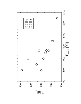
FIG. 1.: RRR_c from all the crystals. The measured residual resistivity ratio for current, $J$, in the $c$-axis direction, $J||c$; along with the equivalent values of RRR_c inferred from the $J||a$ data.

In Fig. 2 we show the resistive transitions of two crystals. The inset shows one of the narrowest resistive transitions measured to date, $\Delta T_{c}=1.3\,\mbox{mK}$, determined as the interval between $10\%$ to $90\%$ of the jump in $\rho_{0}$.

FIG. 2.: Resistivity for a sample annealed at $900^{\rm o}\mbox{C}$ and measured with $J||c$. Inset: Superconducting transition for a sample annealed at $800^{\rm o}\mbox{C}$ with $J||a$ having a transition width of $1.3\,\mbox{mK}$.

The anisotropic resistivity has two components at low temperatures, Fig. 2,

$$\rho_{i}(T)=\rho_{\mbox{0}i}+A_{i}\,T^{2}\,.$$ (1)

The index, $i=(a,c)$, identifies the direction of the current relative to the hexagonal unit cell. The temperature independent term, $\rho_{\mbox{0}i}$, results from elastic scattering of quasiparticles from defects and impurities, and the $T^{2}$ term is due to inelastic scattering, which we assume is a result of quasiparticle-quasiparticle collisions. The coefficient $A_{i}$ is then inversely proportional to the average squared Fermi velocity projected along the direction $i$. As a consequence of the large effective masses, the $A_{i}$ coefficients in heavy fermions are much larger than in conventional metals. The results of our measurements of the anisotropy of the elastic scattering coefficient are presented in Fig. 3. Note that the inelastic coefficients are independent of the residual resistivity, as expected for quasiparticle-quasiparticle scattering with low concentrations of defects and impurities.

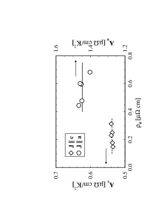
FIG. 3.: Inelastic scattering coefficients for both orientations as a function of $\rho_{\mbox{0}}$.

If the inelastic scattering probability is isotropic, the anisotropy in the angular average of the Fermi velocity can be determined from the $A_{i}$ coefficients,

$$\frac{A_{a}}{A_{c}}=\frac{\langle v_{fc}^{2}(\mathchoice{{\hbox{\boldmath$\displaystyle p$}}}{{\hbox{\boldmath$\textstyle p$}}}{{\hbox{\boldmath$\scriptstyle p$}}}{{\hbox{\boldmath$\scriptscriptstyle p$}}}_{f})\rangle}{\langle v_{fa}^{2}(\mathchoice{{\hbox{\boldmath$\displaystyle p$}}}{{\hbox{\boldmath$\textstyle p$}}}{{\hbox{\boldmath$\scriptstyle p$}}}{{\hbox{\boldmath$\scriptscriptstyle p$}}}_{f})\rangle}=2.69\pm 0.03\,.$$ (2)

The elastic scattering rate can be inferred from the residual resistivities, $\rho_{\mbox{0}i}$, and the Drude result,

$$\rho_{\mbox{0}i}^{-1}=\frac{3}{\pi^{2}}\,\left(\frac{e}{k_{B}}\right)^{2}\gamma_{S}\left<v_{fi}^{2}(\mathchoice{{\hbox{\boldmath$\displaystyle p$}}}{{\hbox{\boldmath$\textstyle p$}}}{{\hbox{\boldmath$\scriptstyle p$}}}{{\hbox{\boldmath$\scriptscriptstyle p$}}}_{f})\,\tau(\mathchoice{{\hbox{\boldmath$\displaystyle p$}}}{{\hbox{\boldmath$\textstyle p$}}}{{\hbox{\boldmath$\scriptstyle p$}}}{{\hbox{\boldmath$\scriptscriptstyle p$}}}_{f})\right>\,,$$ (3)

where $\tau(\mathchoice{{\hbox{\boldmath$\displaystyle p$}}}{{\hbox{\boldmath$\textstyle p$}}}{{\hbox{\boldmath$\scriptstyle p$}}}{{\hbox{\boldmath$\scriptscriptstyle p$}}}_{f})$ is the transport time for quasiparticles scattering into the direction $\mathchoice{{\hbox{\boldmath$\displaystyle p$}}}{{\hbox{\boldmath$\textstyle p$}}}{{\hbox{\boldmath$\scriptstyle p$}}}{{\hbox{\boldmath$\scriptscriptstyle p$}}}_{f}$ on the Fermi surface, and $\gamma_{S}=\frac{2}{3}\pi^{2}k_{B}^{2}N_{f}$ is the Sommerfeld coefficient for the linear term in the electronic specific heat. Thus, the anisotropy in the residual resistivity, $\rho_{\mbox{0}a}/\rho_{\mbox{0}c}$, is determined by the anisotropy in the Fermi velocities and the elastic scattering time. We define effective scattering times for $a$-axis and $c$-axis transport by $\tau_{i}=\big{\langle}v_{fi}^{2}(\mathchoice{{\hbox{\boldmath$\displaystyle p$}}}{{\hbox{\boldmath$\textstyle p$}}}{{\hbox{\boldmath$\scriptstyle p$}}}{{\hbox{\boldmath$\scriptscriptstyle p$}}}_{f})\,\tau(\mathchoice{{\hbox{\boldmath$\displaystyle p$}}}{{\hbox{\boldmath$\textstyle p$}}}{{\hbox{\boldmath$\scriptstyle p$}}}{{\hbox{\boldmath$\scriptscriptstyle p$}}}_{f})\big{\rangle}/\big{\langle}v_{fi}^{2}(\mathchoice{{\hbox{\boldmath$\displaystyle p$}}}{{\hbox{\boldmath$\textstyle p$}}}{{\hbox{\boldmath$\scriptstyle p$}}}{{\hbox{\boldmath$\scriptscriptstyle p$}}}_{f})\big{\rangle}$. For isotropic scattering times the ratio of residual resistivities for $a$-axis and $c$-axis measurements is inversely proportional to the ratio of Fermi-surface averages of the $ab$-plane and $c$-axis Fermi velocities. However, the Fermi velocity anisotropies above cannot account for the anisotropy of $\rho_{\mbox{0}i}$. From our measurements of the suppression of $T_{c}$ as a function of residual resistivity we infer that the elastic scattering rate is anisotropic in UPt₃, i.e.,

$$\frac{\tau_{c}}{\tau_{a}}=\frac{\rho_{\mbox{0}a}\,A_{c}}{\rho_{\mbox{0}c}\,A_{a}}=1.3\pm 0.1\,.$$ (4)

The ratio $\rho_{\mbox{0}a}/\rho_{\mbox{0}c}=3.5\pm 0.3$ used in Eq. (4) is obtained from the slopes of the $T_{c}$ suppression for $a$-axis and $c$-axis currents in Fig. 4. Extrapolation to zero resistivity gives $T_{c0}=563\pm 5\,\mbox{mK}$, where the accuracy is determined by absolute thermometry.

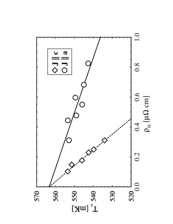
FIG. 4.: $T_{c}$ suppression in UPt₃ vs. the residual resistivity for both orientations. The solid and dashed lines are theoretical fits for an $E_{1g}$ or $E_{2u}$ order parameter (see below).

The basis for this analysis follows from a generalization of the Abrikosov-Gor’kov formula for the pair-breaking suppression of $T_{c}$ to include anisotropic scattering in unconventional superconductors. The suppression of $T_{c}$ by a homogeneous distribution of isotropic, non-magnetic impurities has been calculated for unconventional superconductors,[18] and is given by a formula similar to the Abrikosov-Gor’kov formula for pair-breaking in conventional superconductors by magnetic impurities, i.e., $\ln(T_{c0}/T_{c})=\Psi(\mbox{$1\over 2$}+(\hbar/2\pi\tau k_{B}T_{c}))-\Psi(\mbox{$1\over 2$})$, where $1/\tau$ is the isotropic impurity scattering rate, $T_{c}$ is the superconducting transition temperature, $T_{c0}$ is the transition temperature of the perfect, clean material, and $\Psi$ is the digamma function. This equation, combined with the Drude formula, relates the suppression of $T_{c}$ to the residual resistivity, $\rho_{\mbox{0}}$. We extend this result to include anisotropic scattering in superconductors with an unconventional order parameter and an anisotropic Fermi surface. The simplest model that can account for the observed uniaxial anisotropy of the resistivity is a two parameter model (s-wave and p-wave) for the scattering rate of a quasiparticle with Fermi momentum $\mathchoice{{\hbox{\boldmath$\displaystyle p$}}}{{\hbox{\boldmath$\textstyle p$}}}{{\hbox{\boldmath$\scriptstyle p$}}}{{\hbox{\boldmath$\scriptscriptstyle p$}}}_{f}$ scattering off anisotropic impurities or defects,

$$1/\tau(\mathchoice{{\hbox{\boldmath$\displaystyle p$}}}{{\hbox{\boldmath$\textstyle p$}}}{{\hbox{\boldmath$\scriptstyle p$}}}{{\hbox{\boldmath$\scriptscriptstyle p$}}}_{f})=1/\tau_{\mbox{0}}-3\hat{p}_{fz}^{2}/\tau_{\mbox{1}}\,,$$ (5)

where $\hat{p}_{f}$ is the direction of the Fermi momentum and $1/\tau_{\mbox{0}}\geq 3/\tau_{\mbox{1}}$ guarantees $1/\tau(\mathchoice{{\hbox{\boldmath$\displaystyle p$}}}{{\hbox{\boldmath$\textstyle p$}}}{{\hbox{\boldmath$\scriptstyle p$}}}{{\hbox{\boldmath$\scriptscriptstyle p$}}}_{f})\geq 0$. This model is applicable to anisotropic scattering by a nearly homogeneous distribution of structural defects.[29] The suppression of T_c also depends on the anisotropy of the pairing state. We restrict the analysis to the pairing states that can explain both the H-T phase diagram[4, 13] and the anisotropic thermal conductivity.[15] This restriction allows only the order parameters belonging to the $E_{1g}$ or $E_{2u}$ pairing symmetries, which are the leading candidates for the superconducting phases of UPt₃.[4, 13] The ground state basis functions for these two models are $\eta^{\pm}_{E_{2u}}(\mathchoice{{\hbox{\boldmath$\displaystyle p$}}}{{\hbox{\boldmath$\textstyle p$}}}{{\hbox{\boldmath$\scriptstyle p$}}}{{\hbox{\boldmath$\scriptscriptstyle p$}}}_{f})=\hat{p}_{fz}(\hat{p}_{fx}\pm i\hat{p}_{fy})^{2}$ and $\eta^{\pm}_{E_{1g}}(\mathchoice{{\hbox{\boldmath$\displaystyle p$}}}{{\hbox{\boldmath$\textstyle p$}}}{{\hbox{\boldmath$\scriptstyle p$}}}{{\hbox{\boldmath$\scriptscriptstyle p$}}}_{f})=\hat{p}_{fz}(\hat{p}_{fx}\pm i\hat{p}_{fy})$. The calculation of the suppression of T_c,[18] including anisotropic scattering and anisotropic pairing, gives

$$\ln\frac{T_{c}}{T_{c0}}=\Psi\left(\mbox{$1\over 2$}\right)-{\cal Q}^{-1}\left\langle|\eta(\mathchoice{{\hbox{\boldmath$\displaystyle p$}}}{{\hbox{\boldmath$\textstyle p$}}}{{\hbox{\boldmath$\scriptstyle p$}}}{{\hbox{\boldmath$\scriptscriptstyle p$}}}_{f})|^{2}\Psi\left(\mbox{$1\over 2$}+\mbox{$1\over 2$}\alpha(\mathchoice{{\hbox{\boldmath$\displaystyle p$}}}{{\hbox{\boldmath$\textstyle p$}}}{{\hbox{\boldmath$\scriptstyle p$}}}{{\hbox{\boldmath$\scriptscriptstyle p$}}}_{f})\right)\right\rangle\,,$$ (6)

where $\alpha(\mathchoice{{\hbox{\boldmath$\displaystyle p$}}}{{\hbox{\boldmath$\textstyle p$}}}{{\hbox{\boldmath$\scriptstyle p$}}}{{\hbox{\boldmath$\scriptscriptstyle p$}}}_{f})=\hbar/(2\pi k_{B}T_{c}\tau(\mathchoice{{\hbox{\boldmath$\displaystyle p$}}}{{\hbox{\boldmath$\textstyle p$}}}{{\hbox{\boldmath$\scriptstyle p$}}}{{\hbox{\boldmath$\scriptscriptstyle p$}}}_{f}))$ and ${\cal Q}=\langle|\eta(\mathchoice{{\hbox{\boldmath$\displaystyle p$}}}{{\hbox{\boldmath$\textstyle p$}}}{{\hbox{\boldmath$\scriptstyle p$}}}{{\hbox{\boldmath$\scriptscriptstyle p$}}}_{f})|^{2}\rangle$. For weak scattering Eq. (6) reduces to

$$\frac{T_{c}}{T_{c0}}\simeq 1-\frac{\pi^{2}}{4}{\cal Q}^{-1}\left\langle|\eta(\mathchoice{{\hbox{\boldmath$\displaystyle p$}}}{{\hbox{\boldmath$\textstyle p$}}}{{\hbox{\boldmath$\scriptstyle p$}}}{{\hbox{\boldmath$\scriptscriptstyle p$}}}_{f})|^{2}\alpha(\mathchoice{{\hbox{\boldmath$\displaystyle p$}}}{{\hbox{\boldmath$\textstyle p$}}}{{\hbox{\boldmath$\scriptstyle p$}}}{{\hbox{\boldmath$\scriptscriptstyle p$}}}_{f})\right\rangle\,.$$ (7)

Evaluating the Fermi surface averages for the s-p model gives[30]

$$\frac{T_{c}}{T_{c0}}\simeq 1-\frac{\pi^{2}}{4}q\,\alpha_{0}\,,\quad\alpha_{0}=\frac{\hbar}{2\pi k_{B}T_{c0}\tau_{\mbox{0}}}\,,$$ (8)

where $q=1-1/3r$ for the $E_{2u}$ model and $q=1-3/7r$ for the $E_{1g}$ model. The anisotropy ratio is defined by $r=\tau_{\mbox{1}}/3\tau_{\mbox{0}}$.

Similarly, from the s-p model for the scattering rate and the definition of the effective scattering times, we can relate these to the s-wave and p-wave scattering times,

$$\tau_{a}=\tau_{\mbox{0}}\,\frac{r}{2}\left(1-\left(\sqrt{r}-{1}/{\sqrt{r}}\right)\,\tanh^{-1}\left({1}/{\sqrt{r}}\right)\right)\,,$$ (9)

$$\tau_{c}=\tau_{\mbox{0}}\,r\left(\sqrt{r}\,\tanh^{-1}\left({1}/{\sqrt{r}}\right)-1\right)\,.$$ (10)

These results for $T_{c}/T_{c0}$ and $\tau_{a,c}$ can be combined to express $T_{c}/T_{c0}$ in terms of either $\rho_{\mbox{0}a}$ or $\rho_{\mbox{0}c}$. The slopes, $dT_{c}/d\rho_{\mbox{0}a}=-26.6\pm 2\,\mbox{mK/$\mu\Omega\,$cm}$, $dT_{c}/d\rho_{\mbox{0}c}=-93.0\pm 1\,\mbox{mK/$\mu\Omega\,$cm}$, from Fig. 4 can be used to determine $\tau_{a}$ and $\tau_{c}$, and thus the s- and p-wave scattering times. From the measured anisotropy ratios we obtain $\tau_{c}/\tau_{a}=1.3\pm 0.1$ [Eq. (4)]. The ratio of the s-wave and p-wave scattering rates is then $r\simeq 2$, which corresponds to effective scattering times $\tau_{a}\simeq 1.13\tau_{\mbox{0}}$ and $\tau_{c}\simeq 1.48\tau_{\mbox{0}}$. Combined with the Sommerfeld coefficient, $\gamma_{S}=430\,{\rm mJ\,mol^{-1}\,K^{-2}}$,[9] and Eq. (3), we obtain $\langle v_{f}^{2}(\mathchoice{{\hbox{\boldmath$\displaystyle p$}}}{{\hbox{\boldmath$\textstyle p$}}}{{\hbox{\boldmath$\scriptstyle p$}}}{{\hbox{\boldmath$\scriptscriptstyle p$}}}_{f})\rangle^{1/2}=(2\langle v_{fa}^{2}\rangle+\langle v_{fc}^{2}\rangle)^{1/2}\simeq 3.3\,\mbox{km/s}$. This average is consistent with averaged velocities for extremal orbits obtained from de Haas-van Alphen measurements, $3.5-5.5\,\mbox{km/s}$.[31]

In conclusion we have grown high quality crystals of UPt₃ and have found a means for controlling the elastic scattering by ultra-high vacuum annealing. Using transmission electron microscopy we have identified the defects principally responsible for the scattering as planar defects. We show independently that they are not chemical impurities. The measured suppression of $T_{c}$ with increasing residual resistivity is in good agreement with a simple generalization of the Abrikosov-Gor’kov theory, which includes anisotropic scattering, unconventional pairing, and Fermi surface anisotropy. We infer from the data and this model that the effective scattering rate is approximately $30\%$ weaker for c-axis transport compared with $ab$-plane transport. Finally, we have shown that our crystals approach the perfect, clean limit under appropriate annealing conditions. By extrapolating to zero elastic scattering we deduce the intrinsic transition temperature of UPt₃ to be $563\pm 5\,\mbox{mK}$.

We thank M. Bedzyk, B. Davis and M. Meisel for their contributions to this work and to the heavy fermion research project at Northwestern. The research was supported in part by the NSF (DMR-9705473) Focused Research Grant Program and the NSF (DMR-9120000) Science and Technology Center for Superconductivity and by the NEDO Foundation. Use was made of the Central Facilities of the Northwestern University Materials Research Center supported by NSF (DMR-9120521) MRSEC Program.

REFERENCES

- [1] [†] Present address: Center for Materials Science, Los Alamos National Laboratory, Los Alamos, New Mexico.
- [2] D. Scalapino, Phys. Rep. 250, 239 (1995).
- [3] I. Lee et al., Phys. Rev. Lett. 78, 3555 (1997).
- [4] R. Heffner and M. Norman, Comm. Cond. Matt. Phys. 17, 361 (1996).
- [5] D. Bishop et al., Phys. Rev. Lett. 53, 1009 (1984).
- [6] B. Shivaram et al., Phys. Rev. Lett. 56, 1078 (1986).
- [7] V. Müller et al., Phys. Rev. Lett. 58, 1224 (1987).
- [8] Y. Qian et al. Solid State Commun. 63, 599 (1987).
- [9] R. Fisher et al., Phys. Rev. Lett. 62, 1411 (1989).
- [10] K. Hasselbach, L. Taillefer, and J. Flouquet, Phys. Rev. Lett. 63, 93 (1989).
- [11] G. Bruls et al., Phys. Rev. Lett. 65, 2294 (1990).
- [12] S. Adenwalla et al., Phys. Rev. Lett. 65, 2298 (1990).
- [13] J. Sauls, Adv. Phys. 43, 113 (1994).
- [14] P. Muzikar, D. Rainer, and J. A. Sauls, in Cargese Lectures - 1993 (Kluwer Academic Press, 1993).
- [15] M. J. Graf et al., Phys. Rev. B 53 15147, (1996); J. Low Temp. Phys. 102, 367 (1996); (E) 106, 727 (1997).
- [16] A. A. Abrikosov and L. P. Gor’kov, Sov. Phys. JETP 8, 1090 (1959).
- [17] P. W. Anderson, J. Phys. Chem. Solids 11, 26 (1959).
- [18] L. Gor’kov, Sov. Sci. Rev. A. 9, 1 (1987).
- [19] G.R. Stewart et al., Phys. Rev. Lett. 52, 679 (1984).
- [20] Y. Dalichaouch et al., Phys. Rev. Lett. 75, 3938 (1995).
- [21] T. Vorenkamp et al., Phys. Rev. B 48, 6373 (1993).
- [22] J.B. Kycia et al., J. Low Temp. Phys. 101, 623 (1995); J.B. Kycia, Ph.D thesis, Northwestern University (1997).
- [23] B. E. Warren, X-Ray Diffraction (Addison-Wesley, Reading, MA, 1969).
- [24] A. de Visser, J. Franse, and A. Menovsky, J. Magn. Magn. Mat. 43, 43 (1984).
- [25] N. Kimura et al., J. Phys. Soc. Jpn. 64, 3881 (1995).
- [26] B. Lussier, B. Ellman, and L. Taillefer, Phys. Rev. Lett. 73, 3294 (1994).
- [27] H. Suderow, J. P. Brison, A. Huxley, and J. Flouquet, J. Low Temp. Phys. 108, 11 (1997).
- [28] J. I. Hong, J. B. Kycia, D. Seidman, and W.P. Halperin, to be published.
- [29] M. Franz et al., Phys. Rev. B 56, 7882 (1996); E. Thuneberg et al., Phys. Rev. Lett. 80, 2861 (1998).
- [30] For calculating the Fermi surface averages we mapped an ellipsoidal Fermi surface onto a sphere.
- [31] L. Taillefer and G. Lonzarich, J. Magn. Magn. Mat. 63-64, 372 (1987).