Percolation and lack of self-averaging in a frustrated evolutionary model

Abstract - We present a stochastic evolutionary model obtained through a perturbation of Kauffman’s maximally rugged model, which is recovered as a special case. Our main results are: (i) existence of a percolation-like phase transition in the finite phase space case; (ii) existence of non self-averaging effects in the thermodynamic limit. Lack of self-averaging emerges from a fragmentation of the space of all possible evolutions, analogous to that of a geometrically broken object. Thus the model turns out to be exactly solvable in the thermodynamic limit.

1 Introduction

We present here the analytic study of a model of an abstract behaviour with frustrated rationality. The model, despite or because of its ingenuity, has revealed interesting statistical properties, such as a percolative phase transition in the finite dimensional case and non self-averaging effects in the thermodynamic limit. Our starting point is Kauffman’s well known $NK$ model of biological evolution (see Ref. [1]) in its maximally rugged version ($K=N-1$), whose properties have been extensively investigated. Yet in this paper it serves as a metaphoric abstract model for the behaviour of a fully rational adaptive walker who moves in its phase space in search for an optimal configuration. We decided to perturb its stringent rationality by introducing in the evolutionary rule a probability $p$, as a measure of a certain degree of insanity (or frustration or disorder). For $p=1$ we recover the original model, whereas for $p=0$ we have a random walker in configuration space. The introduction of $p$ is fatal for the adaptive behaviour, but leads to a percolation-like phase transition, that separates a phase characterized by finite walks to optima from one in which the probability of an interminable walk is non zero. We show that in a large configuration space a small perturbation is sufficient to get the percolation threshold. The thermodynamic limit is obtained by letting the cardinality of the phase space go to infinity. We argue that this leads to an infinite number of different possible evolutions. Nevertheless, in this limit we show that the probability $Y$ that two walkers undergo “similar” (in a sense that will become clear later) evolutions has non zero average and a finite variance, that is it lacks of self-averaging. This property will result from a fragmentation of the space of all possible evolutions analogous to that of a geometrically broken object (Ref. [2]).

Evolutionary models have become quite familiar to theoretical physicists, and many of them have been carefully examined (see Refs. [3, 4] for a review). This for two main reasons. (i) Species undergoing biological evolution are dynamical systems, in the sense that their configuration varies with time according to some modelizable dynamical law. The dynamics draws a trajectory in the system’s phase space, that is the set of all possible configurations. (ii) Biological evolution is a complex phenomenon, since one must assume that each step of it derives from and is influenced by the concurrence of different factors, which may be altogether taken into account as a number of random variables that give the system’s trajectory unpredictability and stochasticity. Hence, many ideas taken from the theory of disordered systems, the main of which is that of landscape, may be fruitfully applied for the construction and the study of these seemingly different types of models (see Ref. [5] for a detailed overview).

One assumes that an evolving species (the system) may be found in any of a number of configurations, representing its genome. This is taken for simplicity to be a finite set of spin variables $S_{i}$ ($S_{i}=\pm 1$, $1\leq i\leq N$). The phase space $\Gamma$ is the set $\{+1,-1\}^{N}$ of all genomes. The metric in $\Gamma$ is typically the Hamming distance $d_{H}$. Feature (i) is recovered by giving some evolutionary algorithm $F$ such that

$$\mathcal{C}_{t+1}=F(\mathcal{C}_{t}),$$ (1)

where $\mathcal{C}_{t}$ is the system’s configuration at time $t$ and time is a positive integer or zero. Feature (ii) is introduced through the concept of landscape. For our purposes, a landscape is a pair $(\Gamma,\phi)$, $\Gamma$ being the system’s phase space $\phi$ being a real valued function $\phi:\Gamma\rightarrow\mathbb{R}$ called fitness, defined for all $\mathcal{C}\in\Gamma$. The idea underlying biological evolutionary models is that $F$ lets the system evolve through configurations of growing fitness in search for an optimal one. This optimization procedure is usually not global, that is the system does not seek for the fittest configuration in $\Gamma$; optimal configurations are considered those $x\in\Gamma$ such that $\phi(x)>\phi(y)$, for all $y\in\Gamma$ such that $d_{H}(x,y)=1$. These are called “local optima”.

Of course, the complexity arises from the difficulty in finding the local optima, or, if one wants, from the specific form of $\phi$, which may eventually depend on $t$. The more rugged the landscape, namely the higher the number of maxima and minima of $\phi$, the more complex the dynamics.

In Kauffman’s original idea the fitness of each configuration resulted from epistatic interactions between $K$ of its $N$ genes. An increase of $K$ implied an increase of the number of local fitness optima. This way of tuning the landscape’s complexity is equivalent to the following, which may sound more familiar to physicists (see Ref. [6] for an overview of the contact points between spin glass physics and biology). One assumes that the fitness of a configuration $\mathcal{C}$ is given by a $K$-spin type of hamiltonian,

$$\phi(\mathcal{C})=\sum_{i_{1},\ldots,i_{K}=1}^{N}J_{i_{1},\ldots,i_{K}}S_{i_{1}}\cdots S_{i_{K}},$$ (2)

where $\mathcal{C}=\{S_{1},\ldots,S_{N}\}$ and $J_{i_{1},\ldots,i_{K}}$ are gaussian random variables, with $K\leq N$. It is possible to show (see Refs. [7, 8] for details) that as the parameter $K$ varies from $1$ to $N$ the landscape’s ruggedness grows accordingly, since correlations between the fitness’ values of neighbouring configurations (configurations $x$ and $y$ such that $d_{H}(x,y)=1$) decrease. Therefore for large $K$, that implies large $N$, one finds that the probability $P(\phi_{1},\phi_{2})$ that two configurations $\mathcal{C}_{1}$ and $\mathcal{C}_{2}$ have fitnesses $\phi_{1}\equiv\phi(\mathcal{C}_{1})$ and $\phi_{2}\equiv\phi(\mathcal{C}_{2})$ respectively factorizes:

$$P(\phi_{1},\phi_{2})\simeq P(\phi_{1})P(\phi_{2}).$$ (3)

For all practical purposes $\phi$ behaves thus as a random variable. This is Kauffman’s maximally rugged landscape, which is equivalent to Derrida’s random energy model (again Refs. [7, 8]).

This paper is organized as follows. In Section 2 we give an account of Kauffman’s maximally rugged model, with its main statistical properties. Though much of the material of Section 2 are well-established results, we added them to this paper both to make it self-consistent and to emphasize how the perturbation acts on the system. Section 3 contains the definition of the perturbed model and its analytic study in the finite phase space case. In Section 4 we study the thermodynamic limit. In the final section we make some comments on our results and formulate the conclusions.

2 Kauffman’s maximally rugged model

Kauffman’s maximally rugged model is defined as follows: the system may take on any of the $2^{N}$ configurations of the phase space $\Gamma=\{+1,-1\}^{N}$, and large $N$ is assumed. The fitness $\phi$ is a quenched random variable whose probability density is, say, $p(\phi)$. The dynamics $F$ is then defined as a zero temperature Monte Carlo algorithm:

1. at time $t\geq 0$ the system is in configuration $\mathcal{C}_{t}=\{S_{1},\ldots,S_{N}\}$ with fitness $\phi(\mathcal{C}_{t})$;

2. a spin $S_{i}$ of $\mathcal{C}_{t}$ is chosen at random and its sign is changed, thus obtaining a configuration $\mathcal{C^{\prime}}$ that differs from $\mathcal{C}_{t}$ by just the $i$-th spin ($1\leq i\leq N$);

3. if $\phi(\mathcal{C^{\prime}})>\phi(\mathcal{C}_{t})$ then $\mathcal{C}_{t+1}=\mathcal{C^{\prime}}$; otherwise $\mathcal{C}_{t+1}=\mathcal{C}_{t}$ and return to (ii).

In a rough biological interpretation, this models a situation in which a species evolves increasing its fitness by random point mutations. Trajectories come to an end when the system is in a local fitness maximum, because it cannot find any fitter neighbour. $F$ is a stochastic dynamics that takes the system to such optima passing through configurations of increasing fitness that are just one spin different from one another. The trajectories are usually called adaptive walks, and their length is strictly related to the local properties of the fitness landscape. These have been analytically studied (see Refs. [1] and [9]), revealing a generous structure of very numerous maxima, as we shall soon recall.

Before coming to that, we would like to stress that in what follows we shall consider two types of averages. The first one, which we shall call a “quenched” average, will be denoted by a bar ($\overline{\cdots}$) and indicates averages over all possible fitness realizations. Suppose to be given a certain quantity $q$ (for instance, the number of fitness maxima) that may take on different values in different realizations of $\phi$. The average of $q$ over all possible fitness samplings will be written $\overline{q}$. This notation is slightly unusual since generally this type of average is denoted by brackets. Instead, the second one will be denoted here by brackets ($\langle\ldots\rangle$) and will define averages over many different evolutions. For instance, we shall deal with the average length $\langle\ell\rangle$ of an adaptive walk. This could be written $\langle\ell\rangle=\int\ell dQ(\ell)$, where $Q(\ell)$ is the probability that an adaptive walk consists of $\ell$ steps. In principle it may be difficult to obtain analytical information about the probabilities $Q(x)$ ($x=$ length, duration, …). This average may nevertheless be estimated as follows: one fixes the landscape and averages the lengths of many walks with the same starting point, which by assumption will be the least fit configuration in $\Gamma$. The ensemble in which averages are calculated are thus that of all possible landscapes on $\Gamma$ for $\overline{\cdots}$ and that of all possible evolutions (for example, adaptive walks) for $\langle\ldots\rangle$.

We begin by proving that the average number of local optima increases exponentially with $N$.

Result 1.

Let $f(N)$ denote the fraction of local fitness optima in $\Gamma$ in a given fitness realization (landscape). We have

$$\overline{f(N)}=\frac{1}{N+1}.$$ (4)

The proof is straightforward: let $y(\phi)$ denote the probability that a given configuration has a lower fitness than $\phi$, namely $y(\phi)=\int_{-\infty}^{\phi}p(\phi^{\prime})d\phi^{\prime}$. Since for a local optimum of fitness $\phi$ the $N$ neighbouring configurations must have lower fitness, we have that $\overline{f(N)}$ is the average of $y^{N}$ over all possible choices of $y$. The probability density $q(y)$ of $y$ is uniform, hence

$$\overline{f(N)}=\int_{0}^{1}y^{N}dy=\frac{1}{N+1}.$$ (5)

On the average there are thus $2^{N}/(N+1)$ local optima, so that their number grows exponentially with $N$. Now consider making $\ell$ steps of an adaptive walk starting from the least fit configuration in $\Gamma$. One finds that on the average the probability to take a further step, namely the fraction of fitter neighbours, is halved each time a step is taken.

Result 2.

Let $F(\ell)$ denote the fraction of fitter neighbours after $\ell$ steps. We have

$$\langle F(\ell)\rangle=2^{-\ell}.$$ (6)

Indeed, an adaptive walk can be seen as a sequence of increasing but independent values of $\phi$. If we consider $y(\phi)$ instead of $\phi$, an adaptive walk becomes a sequence of increasing values of $y$, which is, as said above, a random variable with uniform probability density on the $[0,1]$ interval. For one walk of $\ell$ steps, namely for one increasing sequence of $\ell$ independent values $y_{1}$,…,$y_{\ell}$ of $y$, we can write the probability to find an $(\ell+1)$-th value of $y$ greater than all of the previous $\ell$ as

$$F(\ell)=P(y_{2}>y_{1})P(y_{3}>y_{2})\cdots P(y_{\ell+1}>y_{\ell}),$$ (7)

where $P(y_{n}>y_{m})$ denotes the probability of sampling a value $y_{m}$ of $y$ greater than $y_{n}$. $\langle F(\ell)\rangle$ may be obtained by averaging over all possible samplings of $y_{1},\ldots,y_{\ell}$:

$$\langle F(\ell)\rangle=\langle P(y_{2}>y_{1})P(y_{3}>y_{2})\cdots P(y_{\ell+1}>y_{\ell})\rangle.$$ (8)

Clearly, $P(y_{n+1}>y_{n})=1-\int_{0}^{y_{n}}q(y)dy=1-y_{n}$, because $q(y)$ is uniform. Hence

$$\langle F(\ell)\rangle=\langle(1-y_{1})\cdots(1-y_{\ell})\rangle.$$ (9)

The statistical independence of $y_{1},\ldots,y_{\ell}$ implies that

$$\langle F(\ell)\rangle=\langle(1-y_{1})\rangle\cdots\langle(1-y_{\ell})\rangle=\langle(1-y)\rangle^{\ell}.$$ (10)

Now it’s simply $\langle(1-y)\rangle=\int_{0}^{1}(1-y)dy=1/2$ hence the result follows.

Let us now turn to the study of the statistical properties of adaptive walks. The two major outcomes are concerned with the average length of an adaptive walk, which represents the average number of configurations the system has assumed from its starting one to a local fitness maximum, and with the average duration of an adaptive walk, namely the total number of tried mutations, those accepted and those refused.

Result 3.

Let $\langle\ell(N)\rangle$ and $\langle t(N)\rangle$ denote, respectively, the average length and the average duration of an adaptive walk. If $N\gg 1$ we have

1. $\langle\ell(N)\rangle\simeq\log_{2}N$ ;

2. $\langle t(N)\rangle\simeq N$.

1. is an estimate for $\langle\ell(N)\rangle$. It is obtained through the consideration that an adaptive walk ends when the fraction $F(\ell)$ of fitter neighbours falls below $1/N$. Hence the average length is that for which $\langle F(\ell)\rangle\simeq\frac{1}{N}$. From Result 2 one soon gets

$$2^{-\ell}\simeq\frac{1}{N},$$ (11)

whence the estimate $\langle\ell(N)\rangle\simeq\log_{2}N$ follows. A more rigorous though much more complicated estimate has been derived in Ref. [10], where it is shown that $\langle\ell(N)\rangle\simeq\log N$ with a proportionality constant that is slightly different from $(\log 2)^{-1}$. Therefore it is reasonable to take 1. as a fairly good estimate.

For what concerns 2., we consider that since the fraction of fitter neighbours is halved on the average at each step, then the waiting time (if one wants, the number of tried and refused mutations) doubles on the average at each step. So the average number of time units one has to wait in order to take the $\ell$-th step is $2^{\ell-1}$ (one has to wait a time $1$ to take the first step because by assumption each walk starts from the least fit configuration in $\Gamma$). We obtain $\langle t(N)\rangle$ by summing all waiting times in each configuration passed by in an adaptive walk, the average number of which is given by 1.; hence

$$\langle t(N)\rangle=\sum_{\ell=1}^{\log_{2}N}2^{\ell-1}=N-1,$$ (12)

where the sum has been performed as if $\log_{2}N$ were an integer. For large $N$ 2. is recovered. Again, in Ref. [10] it is shown that a more rigorous derivation of $\langle t(N)\rangle$ yields the same result $\langle t(N)\rangle\simeq N$ up to a proportionality constant that is just slightly different from $1$. Therefore 2. may well be considered a good estimate.

3 Perturbing Kauffman’s model

In the previous section we have recalled the statistical properties of Kauffman’s maximally rugged model. Following its dynamical rule $F$ the system can evolve only through fitter configurations. In some sense, looking back at spin glasses, one could say that it lacks of frustration. The system always does the right thing, always finds its way in the rugged landscape, in a finite number of steps reaches a fitness maximum, and that’s it; failures are ruled out. In our perturbed version of this model we want to frustrate the rationality of the system with an additive selective pressure $p$, acting as a constraint on the system’s optimizing ability.

We thus consider a system whose phase space is $\Gamma=\{+1,-1\}^{N}$, evolving in a landscape where the fitness $\phi$ is a quenched random variable. The law of evolution $F_{p}$ depends on a real parameter $p\in[0,1]$ through the following definition:

1. at time $t\geq 0$ the system is in configuration $\mathcal{C}_{t}=\{S_{1},\ldots,S_{N}\}$ with fitness $\phi(\mathcal{C}_{t})$;

2. a spin $S_{i}$ of $\mathcal{C}_{t}$ is chosen at random and its sign is changed, thus obtaining a configuration $\mathcal{C^{\prime}}$ that differs from $\mathcal{C}_{t}$ by just the $i$-th spin ($1\leq i\leq N$);

3. if $\phi(\mathcal{C^{\prime}})>\phi(\mathcal{C}_{t})$ then, with probability $p$, $\mathcal{C}_{t+1}=\mathcal{C^{\prime}}$ and, with probability $1-p$, $\mathcal{C}_{t+1}$ is chosen at random among the $N$ neighbouring configurations of $\mathcal{C}_{t}$;

4. if $\phi(\mathcal{C^{\prime}})<\phi(\mathcal{C}_{t})$, then $\mathcal{C}_{t+1}=\mathcal{C}_{t}$ and return to (ii).

The landscape’s statistical properties are the same as those of Kauffman’s model, so that Result 1 still holds. The difference with the original model is that this time the system accepts a favourable mutation only with a probability $p$. If it can not, then it is forced to choose a random spin and change its sign, regardless of the fitness of this newly-obtained configuration. By this we mean to model a system that undergoes an external evolutionary pressure, whose strength increases with $p$ varying from $1$ to $0$, as it evolves in a rugged landscape. The pressure is a perturbation of the dynamics, such that the case $p=1$ corresponds to the unperturbed model. We’ll see that a small perturbation is sufficient to drastically change all statistical properties of the model. For example, the average length of a trajectory, which we shall call a p-walk, diverges.

Let us consider the case of finite $N$. We begin by deriving the analogous for the perturbed model of Result 2 for the unperturbed one.

Result 4.

Let $F_{p}(\ell)$ denote the fraction of fitter neighbours after $\ell$ steps of a $p$-walk and let $\langle F_{p}(\ell)\rangle\equiv\langle F(\ell)\rangle_{p}$. We have

$$\langle F(\ell)\rangle_{p}=\frac{1}{2-p}\bigg{(}\Big{(}\frac{p}{2}\Big{)}^{\ell}+1-p\bigg{)}.$$ (13)

One sees that in the $p\rightarrow 1$ limit, Result 2 is recovered.

The proof is not difficult but tedious. Observe that at each mutation the system makes a choice between two symbols: $p$ and $1-p$. Let $\Omega$ denote the set of all possible sequences of choices the system can make in a $p$-walk of given length $\ell$, namely $\Omega=\{p,1-p\}^{\ell}$. One can think of a $p$-walk $\omega$ of $\ell$ steps as an element of $\Omega$ of the form

$$\omega=\{\omega_{1},\ldots,\omega_{\ell}\},$$ (14)

where $\omega_{j}\in\{p,1-p\}$ for $1\leq j\leq\ell$. We shall call $\Omega$ the “space of $p$-walks”. Considering that when the system accepts a positive mutation the average fraction of fitter neighbours is halved, one can construct a partition of $\Omega$ made by subsets of “similar” $p$-walks:

1. the first subset $\Omega_{1}$ contains those $p$-walks such that $\omega_{\ell}=1-p$;

2. the second subset $\Omega_{2}$ contains those $p$-walks such that $\omega_{\ell-1}=1-p$ and $\omega_{\ell}=p$;

3. the $k$-th subset ($1\leq k\leq\ell-1$) $\Omega_{k}$ contains those $p$-walks such that $\omega_{\ell-k+1}=1-p$ and $\omega_{\ell-k+2},\ldots,\omega_{\ell}=p$;

4. the $\ell$-th subset $\Omega_{\ell}$ contains the $p$-walks $\{1-p,p,\ldots,p\}$ e $\{p,\ldots,p\}$.

We shall call “types” of $p$-walks the subsets $\Omega_{m}$ ($m=1,\ldots,\ell$), so that a $p$-walk $\omega\in\Omega_{m}$ is a $p$-walk of the $m$-th type. The similarity consists of the fact that all $p$-walks of the $m$-th type are such that, on the average, after the $\ell$-th step there is a fraction of $2^{-m}$ fitter neighbours than the configuration reached by the system. This is so because this average fraction depends on how many $p$-steps (steps in which the mutation has been accepted) the system has made since the last $(1-p)$-step. In fact, a $(1-p)$-step brings the system to a configuration having, on the average, a fraction of $1/2$ fitter neighbours (if $N$ is sufficiently large) and each $p$-step following halves this fraction. For example, if $n-1$ $p$-steps are taken after a $(1-p)$-step (namely if a $p$-walk of the $n$-th subset is made), the average fraction of fitter neighbours will be $2^{-n}$. So the probability to have $2^{-m}\cdot N$ fitter neighbours after $\ell$ steps equals the probability $P(\Omega_{m})$ to take a $p$-walk of the $m$-th type. This is easily calculated: the probability $P(\omega)$ that the $p$-walk $\omega=\{\omega_{1},\ldots,\omega_{\ell}\}$ is made is simply

$$P(\omega)=\prod_{i=1}^{\ell}\omega_{i}$$ (15)

and thus

$$P(\Omega_{m})=\sum_{\omega\in\Omega_{m}}P(\omega).$$ (16)

A straightforward calculation shows that

$$P(\Omega_{\ell}) =p^{\ell-1}$$ (17)

$$P(\Omega_{k}) =(1-p)p^{k-1}$$ (18)

with $1\leq k\leq\ell-1$. Hence $\langle F(\ell)\rangle_{p}$ may be derived from the formula

$$\langle F(\ell)\rangle_{p}=\sum_{m=1}^{\ell}P(\Omega_{m})2^{-m},$$ (19)

that makes use of the fact that the average fraction of fitter neighbours is $2^{-m}$ with probability $P(\Omega_{m})$ (namely, when the walk done is of the $m$-th type), and of the fact that, clearly,

$$\sum_{m=1}^{\ell}P(\Omega_{m})=1.$$ (20)

We rewrite formula (19) explicitly:

$$\langle F(\ell)\rangle_{p}=p^{\ell-1}2^{-\ell}+\sum_{k=0}^{\ell-2}(1-p)p^{k}2^{-(k+1)}.$$ (21)

Performing the sum and with a minor rearrangement of the terms Result 4 is obtained.

Result 4 is the starting point for deriving an estimate for the average length $\langle\ell(N)\rangle_{p}$ of a $p$-walk. It is sufficient to consider that on the average the walk stops when $\langle F(\ell)\rangle_{p}$ falls below the value $\frac{1}{N}$, that is, when there are no fitter neighbours. Hence the stopping condition reads

$$\langle F(\ell)\rangle_{p}\sim\frac{1}{N},$$ (22)

which leads to

$$\Big{(}\frac{p}{2}\Big{)}^{\ell}+1-p\sim\frac{2-p}{N}.$$ (23)

Isolating $\ell$ from the previous formula is a simple task and one obtains

$$\langle\ell(N)\rangle_{p}\simeq\log_{\frac{p}{2}}\Big{[}\frac{1}{N}\big{(}(N-1)p-(N-2)\big{)}\Big{]}.$$ (24)

One sees that in the $p\rightarrow 1$ limit the average length of an adaptive walk is recovered:

$$\langle\ell(N)\rangle_{1}\equiv\langle\ell(N)\rangle\simeq\log_{2}N.$$ (25)

Formula (24) may be put in a more fashionable way as is shown by the following result, analogous to Result 3 of the unperturbed model.

Result 5.

Let $\langle\ell(N)\rangle_{p}$ and $\langle t(N)\rangle_{p}$ denote, respectively, the average length and duration of a $p$-walk. There exists an $N$-dependent number $p_{c}\in]0,1[$ such that the following estimates hold:

1. $$\langle\ell(N)\rangle_{p}\simeq\frac{\log\Big{[}\frac{1}{N}\big{(}(p-p_{c}(N))(N-1)\big{)}\Big{]}}{\log\frac{p}{2}};$$ (26)

2. $$\langle t(N)\rangle_{p}\simeq\frac{1}{1-2p}\bigg{(}(1-p)\langle\ell(N)\rangle_{p}-p\frac{1-(2p)^{\langle\ell(N)\rangle_{p}}}{1-2p}\bigg{)}.$$ (27)

Let us rewrite formula (24) in the form

$$\langle\ell(N)\rangle_{p}\simeq\frac{\log\Big{[}\frac{1}{N}\big{(}(N-1)p-(N-2)\big{)}\Big{]}}{\log\frac{p}{2}}.$$ (28)

This must by definition be a positive number, though it may not be an integer. But since its denominator is negative, so has to be its numerator. But this only holds if

$$0<\frac{1}{N}\big{(}(N-1)p-(N-2)\big{)}<1.$$ (29)

The right side inequality leads to a condition for $p$ that is always satisfied; the left inequality leads on the contrary to the requirement that

$$p>p_{c}(N)=1-\frac{1}{N-1}.$$ (30)

Minor rearrangements of the terms in formula (24) lead thus to part 1. of Result 5.

We see now from formula (26) that the average length of a $p$-walk diverges as $p\rightarrow p_{c}(N)^{+}$. Note that the critical threshold $p_{c}$ depends on the dimension $N$ of the phase space. Also, it is simple to check that, for all $N$,

$$\lim_{p\rightarrow p_{c}^{+}}\frac{\langle\ell(N)\rangle_{p}}{\log(p-p_{c})}=\beta<0.$$ (31)

This means that when we approach the critical point from above the average length diverges as

$$\langle\ell(N)\rangle_{p}\approx\log(p-p_{c})^{\beta}=-|\beta|\log(p-p_{c}).$$ (32)

Let us turn to time. It is clear that a $p$-walk of infinite length is also of infinite duration. Reminding that one unit of time corresponds to a trial spin flip and fitness check in our model, let us derive an expression for the average duration $\langle t(N)\rangle_{p}$ of a $p$-walk. The strategy we wish to adopt is the following: since the system remains for a certain amount of time in each configuration it visits, during which it tries point mutations to find a fitter neighbour, we can think of evaluating the average time spent in a configuration, and sum over all configurations visited during a $p$-walk, that on the average are $\langle\ell(N)\rangle_{p}$. In the case of an adaptive walk everything’s simple: since the fraction of fitter neighbours is halved on the average at each step, the waiting time is doubled on the average, so that in order to take the $\ell$-th step it is necessary to wait a time $\langle\tau(\ell)\rangle=2^{\ell-1}$ on the average (the average waiting time to take the first step is one since all neighbours are fitter by assumption, and so on).

Hence, when the average fraction of fitter neighbours is $2^{-\ell}$ the time required on the average to find a fitter one mutant configuration is $2^{\ell-1}$. We thus could estimate the average waiting time $\langle\tau(\ell)\rangle_{p}$ to take the $\ell$-th step of a $p$-walk as we did estimate $\langle F(\ell)\rangle_{p}$, namely by formula (19), just by substituting all average fractions of fitter neighbours $2^{-\ell},\ldots,2^{-1}$ with the corresponding average waiting times $2^{\ell-1},\ldots,1$. We have

$$\langle\tau(\ell)\rangle_{p}=\sum_{m=1}^{\ell}P(\Omega_{m})2^{m-1};$$ (33)

using the probabilities (17) we obtain immediately

$$\langle\tau(\ell)\rangle_{p}=p^{\ell-1}2^{\ell-1}+(1-p)\sum_{k=0}^{\ell-2}p^{k}2^{k}.$$ (34)

Performing the sum we finally arrive at

$$\langle\tau(\ell)\rangle_{p}=\frac{1}{1-2p}\Big{(}1-p-p(2p)^{\ell-1}\Big{)},$$ (35)

which is what we were looking for. One sees that in the no-perturbation limit $p\rightarrow 1$ this result leads to $\langle\tau(\ell)\rangle_{1}=2^{\ell-1}$, as we expected. Furthermore, note that for $\ell=1$ we get $\langle\tau(1)\rangle_{p}=1$ for every $p$, which is right since in this model also the time needed to take the first step is one.

Summing over all configurations transversed during a $p$-walk on the average we obtain an estimate for the average duration $\langle t(N)\rangle_{p}$:

$$\langle t(N)\rangle_{p}\simeq\sum_{\ell=1}^{\langle\ell(N)\rangle_{p}}\langle\tau(\ell)\rangle_{p}=\sum_{\ell=0}^{\langle\ell(N)\rangle_{p}-1}\langle\tau(\ell)\rangle_{p}.$$ (36)

The last equality holds by virtue of the fact that in formula (35) the dependence on $\ell$ is only in the term $(2p)^{\ell-1}$. Therefore we may redefine $\ell$ (ranging from $1$ to $\langle\ell(N)\rangle_{p}$) as $\ell-1$, and this new variable varies from $0$ to $\langle\ell(N)\rangle_{p}-1$. After a minor rearrangement of the terms we see we can split the sum in two sums:

$$\langle t(N)\rangle_{p}\simeq\frac{1}{1-2p}\Bigg{(}\sum_{\ell=0}^{\langle\ell(N)\rangle_{p}-1}(1-p)-p\sum_{\ell=0}^{\langle\ell(N)\rangle_{p}-1}(2p)^{\ell}\Bigg{)}.$$ (37)

Now perform the sums under the assumption that $\langle\ell(N)\rangle_{p}$ is an integer (we are interested in an estimate; if the average length were not an integer, we would get an estimate by summing up to $\lfloor\langle\ell(N)\rangle_{p}\rfloor$):

$$\langle t(N)\rangle_{p}\simeq\frac{1}{1-2p}\bigg{(}(1-p)\langle\ell(N)\rangle_{p}-p\frac{1-(2p)^{\langle\ell(N)\rangle_{p}}}{1-2p}\bigg{)},$$ (38)

which is the estimated average duration of a $p$-walk. Note that in the $p\rightarrow 1$ limit, where $\langle\ell(N)\rangle_{p}\rightarrow\log_{2}N$, one recovers

$$\langle t(N)\rangle_{1}\equiv\langle t(N)\rangle\simeq N-1,$$ (39)

that in the large $N$ limit is what one gets from Kauffman’s maximally rugged model.

We have thus discovered that if $p>p_{c}(N)$ then the average length of a $p$-walk in the rugged random landscape is finite, whereas at $p=p_{c}(N)$ $\langle\ell(N)\rangle_{p}$ diverges. We emphasize that this picture is qualitatively correct, despite of the fact that formula (26) is an estimate for $\langle\ell(N)\rangle$. The critical probability $p_{c}(N)$ depends on the phase space’s dimension $N$. If $N$ is large, as we have assumed to derive these formulas, then it is close to one. Thus a small perturbation, which means a value of $p$ which is just slightly different from $1$, is sufficient to switch on the probability that the system wanders through the rugged landscape indefinitely.

In effect, we can render these observations more quantitative.

Result 6.

Let $Q_{p}(\ell)$ denote the probability that a $p$-walk consists of $\ell$ steps. We have

$$Q_{p}(\infty)\begin{cases}=0&\text{for $p>p_{c}(N)$};\\ >0&\text{for $p<p_{c}(N)$}.\end{cases}$$ (40)

Of course we assume the validity of the normalization condition

$$Q_{p}(\infty)+\sum_{\ell=1}^{\infty}Q_{p}(\ell)=1,$$ (41)

that should hold for all $p\in[0,1]$ and where we have separated the term corresponding to $\ell=\infty$. To prove Result 6 it is sufficient to put $\langle\ell(N)\rangle_{p}$ in the form

$$\langle\ell(N)\rangle_{p}=\infty Q_{p}(\infty)+\sum_{\ell=1}^{\infty}\ell Q_{p}(\ell),$$ (42)

and consider that this average value is finite whenever $p>p_{c}(N)$, and infinite otherwise.

We have mutuated this fancy way of writing this average value from percolation theory, where the average number of lattice points in a cluster $\langle n\rangle_{p}$ is written as (see for example Ref. [11], where $\langle n\rangle_{p}\equiv\chi(p)$)

$$\langle n\rangle_{p}=\infty P_{p}(\infty)+\sum_{n=1}^{\infty}nP_{p}(n),$$ (43)

where $P_{p}(n)$ represents the probability that a cluster contains exactly $n$ points. Equations (42) and (43) are not very satisfactory from a notation point of view, since the quantity $\infty$ is treated like a number. Anyhow, equation (40) indicates that this $p$-walks’ model displays a percolation-like transistion, that is just analogous to the one described by

$$P_{p}(\infty)\begin{cases}=0&\text{for $p<p_{c}(N)$};\\ >0&\text{for $p>p_{c}(N)$},\end{cases}$$ (44)

which characterises “classical” percolation theory, where $N$ indicates the dimensionality of the lattice one is considering. In the large $N$ limit of the $p$-walks’ model the percolation threshold is close to $1$ (see formula (30)), so that a small perturbation is enough to turn on the probability of no arrest.

4 The thermodynamic limit

The thermodynamic limit is obtained by letting the dimension $N$ of the phase space $\Gamma=\{+1,-1\}^{N}$ to infinity. In this limit the average length of an adaptive walk diverges logarithmically as stated by Result 3. Hence, all $p$-walks are interminable. It is therefore natural to consider, together with the $N\rightarrow\infty$ limit for $\Gamma$, the $\ell\rightarrow\infty$ limit for $\Omega=\{p,1-p\}^{\ell}$.

In the previous section we have seen that for finite $\ell$ $\Omega$ may be fragmented into $\ell$ subsets which we called “types” of $p$-walks. All walks of the same type, say the $m$-th ($1\leq m\leq\ell$), are such that, on the average, after $\ell$ steps the fraction of fitter neighbours or, if one wants, the probability to take one further step is $2^{-m}$. We have denoted by $\Omega_{m}$ the $m$-th type and by $P(\Omega_{m})$ the probability that a $p$-walk is of the $m$-th type. We have then found that $P(\Omega_{k})=(1-p)p^{k-1}$ for $k=1,\ldots,\ell-1$, and that $P(\Omega_{\ell})=p^{\ell-1}$. When $\ell$ goes to infinity the number of fragments in which the $\Omega$ space is broken diverges, but still each fragment retains the same meaning, for the probability that a certain $p$-walk is of a given type does not change if the number of types diverges. For example, the probability that a $p$-walker finds half of his neighbours fitter than him after $\ell$ steps is always $1-p$ for all $\ell$. What happens is just that when the walker takes an $(\ell+1)$-th step an additional type (the $(\ell+1)$-th) must be taken into account. But its probability $P(\Omega_{\ell+1})$ causes a change in $P(\Omega_{\ell})$, whereas the probabilities of the remaining types are unchanged.

Hence, $\Omega$’s thermodynamic limit may be thought of as if it were constructed as follows. Take $\Omega$ as an object of size $P(\Omega)=1$ and suppose to break it into infinite pieces $\Omega_{1},\Omega_{2},\ldots$ of sizes $W_{1}=P(\Omega_{1}),W_{2}=P(\Omega_{2}),\ldots$ respectively. The breaking process depends on a given real number $p\in[0,1]$. First, we tear $\Omega$ in two pieces of sizes $W_{1}=1-p$ and $p$. Then we take the latter and tear it in two pieces of sizes $W_{2}=(1-p)p$ and $p^{2}$. Thirdly, we take the one of size $p^{2}$ and break it in two pieces of sizes $W_{3}=(1-p)p^{2}$ and $p^{3}$. In principle, one may continue breaking the pieces of sizes $p^{\ell+1}$ at the $\ell$-th step and take the $\ell\rightarrow\infty$ limit. In the end we have an infinite set of pieces of sizes

$$W_{1} =1-p$$

$$W_{2} =(1-p)p$$

$$\ldots$$ (45)

$$W_{s} =(1-p)p^{s-1}$$

$$\ldots$$

The sizes $W_{s}$ represent the probability that a $p$-walk is of the $s$-th type in the thermodynamic limit. Clearly, $\sum_{s}W_{s}=\sum_{s=1}^{\infty}(1-p)p^{s-1}=1$. In Ref. [2] we called this a geometrically broken object, since the sizes of the resulting pieces form a geometric sequence. In fact, $W_{s+1}=pW_{s}$ for $s=1,2,\ldots$ .

Now suppose to be given a certain number of $p$-walkers, each of which chooses his value of $p$ from a given probability density $\rho(p)$ on the $[0,1]$ interval. To each of these will correspond a specific rupture of the space $\Omega$ of $p$-walks, since for the geometrical breaking the weights of the types $W_{s}$ depend just on the value of $p$. Hence each $p$-walker gives a breaking sample of $\Omega$. This picture is quite usual in the theory of disordered systems, where one deals with systems having a quenched disorder represented by a number of stationary random variables. For each sample, namely for each choice of the quenched disorder, certain statistical or thermodynamic extensive obsevables $X$ (for example, the free energy density) may be evaluated. One is usually interested in averaging $X$ over disorder, i.e. over all possible samplings of the quenched random variables. The most interesting outcome in many cases is that non self-averaging effects are present: sample-to-sample fluctuations of $X$ do not vanish in the thermodynamic limit (i.e. when one lets the size of the sistem go to infinity). This means that $\langle X\rangle$ (the average of $X$ over disorder) is finite and that $\textrm{var}(X)=\langle X^{2}\rangle-\langle X\rangle^{2}$ is non zero. The probability density $P(X)$ of $X$ remains “broad” in the thermodynamic limit, whereas for a self-averaging quantity the probability density in the same limit is highly concentrated around its average. As a result, the value of a self-averaging quantity on a sufficiently large sample is a good estimate of the ensemble average, while for non self-averaging quantities no sample, no matter how large, is a good representative of the whole ensemble.

More specifically, in model broken objects as the randomly broken object [12] as well as in other more complicated models (see Ref. [13] for a unifying review) one finds that the sizes $W_{s}$ of the pieces lack of self-averaging. In all of these the thermodynamic limit is obtained by letting the number of pieces go to infinity. The study of non self-averaging properties of a geometrically broken object is the content of Ref. [2]. The model turns out to be exactly solvable.

We consider in each sample the probability

$$Y=\sum_{s}W_{s}^{2}$$ (46)

that two randomly chosen walks in $\Omega$ are of the same type. The aim is to show that $Y$’s ensemble average $\langle Y\rangle$ over disorder (that is, over $p$) is non zero and that $Y$’s variance $\textrm{var}(Y)=\langle Y^{2}\rangle-\langle Y\rangle^{2}$ does not vanish. This would yield the conclusion that the probabilities $W_{s}$ of the types are non self-averaging quantities. Among other results, in Ref. [2] we have proved that

1. the probability density $\Pi(Y)$ of $Y$ over all possible samples of a geometrically broken object is given in the thermodynamic limit by

   $$\Pi(Y)=\frac{2}{(1+Y)^{2}}\rho\bigg{(}\frac{1-Y}{1+Y}\bigg{)}.$$ (47)

2. Assuming $\rho(p)=1$ the ensemble average of $Y$ is given by

   $$\langle Y\rangle=\int_{0}^{1}Y\Pi(Y)dY=\log 4-1\simeq 0.386\ldots.$$ (48)

3. Under the same assumption one can calculate the second moment $\langle Y^{2}\rangle$ of $Y$ and show that the variance is given by

   $$\textrm{var}(Y)=\langle Y^{2}\rangle-\langle Y\rangle^{2}\simeq 0.078\ldots.$$ (49)

We thus come to the interesting conclusion that in the thermodynamic limit of the $p$-walks’ model non self-averaging effects are present: the probabilities that a $p$-walk is of a given type lack of self-averaging (i.e. they remain sample dependent). In other terms, the probability $Y$ that two $p$-walkers with same $p$ make walks of the same type has non zero average and finite variance, despite of the fact that there are infinite different types.

Let us now turn to a different problem. Consider two $p$-walkers with freedom parameters $p_{1}$ and $p_{2}$ respectively. We know that for each of them the probability that a $p$-walk is of the $s$-th type is given by $W_{s}(p_{i})=(1-p_{i})p_{i}^{s-1}$, for $i=1,2$. Let us define the variable

$$Z\equiv Z(p_{1},p_{2})=\sum_{s}W_{s}(p_{1})W_{s}(p_{2}),$$ (50)

giving the probability that a randomly chosen $p_{1}$-walk and a randomly chosen $p_{2}$-walk in $\Omega$ are of the same type. The ensemble average $\langle Z\rangle$ has to be evaluated over all possible choices of $p_{1}$ and $p_{2}$. $\langle Z\rangle$ has some resemblence with a correlation function in the space $\Omega$ of $p$-walks. We shall now prove that it is possible to calculate the probability density $\Phi(Z)$ of $Z$, such that the probability that for a given choice of $p_{1}$ and $p_{2}$ $Z$ is in the $[Z,Z+dZ]$ interval is given by $\Phi(Z)dZ$. More precisely we prove the following:

Result 7.

If both $p_{1}$ and $p_{2}$ are chosen from a uniform probability density on the $[0,1]$ interval, then the probability density $\Phi(Z)$ of $Z$ is given by

$$\Phi(Z)=\frac{2}{(1+Z)^{3}}\big{(}1-Z^{2}-2Z\log Z\big{)}.$$ (51)

This allows us to evaluate $\langle Z\rangle$ and $\textrm{var}(Z)=\langle Z^{2}\rangle-\langle Z\rangle^{2}$. One finds that

$$\langle Z\rangle =\int_{0}^{1}Z\Phi(Z)dZ\simeq 0.289867\ldots$$ (52)

$$\langle Z^{2}\rangle =\int_{0}^{1}Z^{2}\Phi(Z)dZ\simeq 0.130395\ldots$$ (53)

$$\textrm{var}(Z) \simeq 0.04637\ldots$$ (54)

This tells us that, like $Y$, $Z$ is non self-averaging. But it also tells us that the values of $Z$ are more concentrated around its average than those of $Y$, at least for uniform $\rho$, since $\textrm{var}(Z)$ is smaller than $\textrm{var}(Y)$.

We begin by calculating $Z$ for two given values of $p_{1}$ and $p_{2}$. One has

$$Z=\sum_{s=1}^{\infty}(1-p_{1})p_{1}^{s-1}(1-p_{2})p_{2}^{s-1}=(1-p_{1})(1-p_{2})\sum_{s}(p_{1}p_{2})^{s-1},$$ (55)

whence

$$Z(p_{1},p_{2})=\frac{(1-p_{1})(1-p_{2})}{1-p_{1}p_{2}}.$$ (56)

For simplicity of notation set $p_{1}=x$ and $p_{2}=y$. Let

$$\zeta(x,y)=\frac{(1-x)(1-y)}{1-xy}$$ (57)

and define the region $D(Z)\subseteq[0,1]^{2}$

$$D(Z)=\{(x,y)\in[0,1]^{2}:(\zeta(x,y)\leq Z)\wedge(Z\in[0,1])\}.$$ (58)

Suppose that $x$ and $y$ are random variables with probability distributions $\rho(x)$ and $\rho(y)$. The probability $\mathsf{P}\{\zeta(x,y)\leq Z\}\equiv F(Z)$ is simply

$$F(Z)=\int\!\!\!\int_{D(Z)}\rho(x)\rho(y)dxdy.$$ (59)

$F(Z)$ and $\Phi(Z)$ are related by

$$\Phi(Z)=\frac{dF(Z)}{dZ}$$ (60)

therefore calculating $F(Z)$ is the crucial step towards $\Phi(Z)$. Suppose for simplicity that $\rho=1$, so that $F(Z)$ is the area of $D(Z)$. From definition (57) we see that for $x=0$ $\zeta(0,y)=1-y$. Hence the curve $\zeta(x,y)=Z$ touches the $y$ axis in the point $y_{0}=1-Z$. We thus construct the rectangle $R(Z)=[y_{0},1]\times[0,1]$ (as shown in Figure 1) and note that it is contained in $D(Z)$. $F(Z)$ may thus be separated as

$$F(Z)=\int\!\!\!\int_{R(Z)}dxdy+\int\!\!\!\int_{D(Z)\setminus R(Z)}dxdy.$$ (61)

The first integral is equal to the area of $R(Z)$, that is $Z$. For what concerns the second integral, we choose to evaluate it for $x$ running on the curve $\zeta(x,y)=Z$ and $y$ ranging from $0$ to $y_{0}=1-Z$. The coordinates $x$ of the points on the curve $\zeta(x,y)=Z$ have the form

$$x(y,Z)=\frac{y+Z-1}{y(Z+1)-1},$$ (62)

as can be seen by inversion of definition (57). Therefore

$$\int\!\!\!\int_{D(Z)\setminus R(Z)}dxdy=\int_{0}^{1-Z}dy\int_{x(y,Z)}^{1}dx=\int_{0}^{1-Z}\big{(}1-x(y,Z)\big{)}dy.$$ (63)

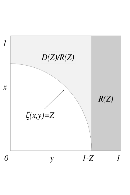
Figure 1: Regions $R(Z)$ and $D(Z)\setminus R(Z)$.

We thus need to calculate the integral

$$\int\!\!\!\int_{D(Z)\setminus R(Z)}dxdy=\int_{0}^{1-Z}\Bigg{(}1-\frac{y+Z-1}{y(Z+1)-1}\Bigg{)}dy.$$ (64)

This is a quite simple task, and the result is

$$\int\!\!\!\int_{D(Z)\setminus R(Z)}dxdy=\frac{Z}{(1+Z)^{2}}\big{(}1-Z^{2}-2Z\log Z\big{)}.$$ (65)

We finally obtain $F(Z)$ from identity (61):

$$F(Z)=\frac{2Z}{(1+Z)^{2}}\big{(}1+Z(1-\log Z)\big{)}.$$ (66)

Differentiating this with respect to $Z$ we get at last Result 7:

$$\Phi(Z)=\frac{2}{(1+Z)^{3}}\big{(}1-Z^{2}-2Z\log Z\big{)}.$$ (67)

5 Conclusion

To summarize we have studied an abstract evolutionary model in which the system’s size is $N$ and phase space $\Gamma$ has $2^{N}$ configurations. The evolutionary rule $F_{p}$ is a stochastic map that depends on a real parameter $p\in[0,1]$. For $p=1$ we recover Kauffman’s maximally rugged model and trajectories to local fitness optima are adaptive walks. For generic $p$ we have introduced $p$-walks. In the finite $N$ case we have shown that the average length of a $p$-walk as estimated by Result 5 is finite whenever $p>p_{c}(N)$, where the critical value $p$ is given by $p_{c}(N)=1-1/(N-1)$. When $p\rightarrow p_{c}(N)^{+}$ and for all $p<p_{c}(N)$ the average length diverges. This results in a percolation-like phase transition. In the supercritical phase ($p>p_{c}(N)$) all $p$-walks are of finite length, whereas in the subcritical phase ($p<p_{c}(N)$) the probability of an infinitely long $p$-walk is non zero. In the thermodynamic limit $N\rightarrow\infty$ we have emphasized the fact that the dimension of the space $\Omega$ of $p$-walks must be considered infinite. $\Omega$ contains all representations of $p$-walks of a given length, hence the thermodynamic limit yields a divergence in the number of different possible evolutions. We have shown that $\Omega$ may be partitioned in infinite subsets grouping “similar” $p$-walks. This fragmentation is analogous to that of a geometrically broken object. Hence, we were able to prove that non self-averaging effects are present: the probability $Y$ that two $p$-walkers with same value of $p$ have similar evolutions has non zero average and finite variance, even though the number of different types of evolutions is infinite. Lastly, we have studied the probability $Z$ that two different $p$-walkers (with different values of $p$) have similar evolutions and have shown that $Z$ is also non self-averaging. The simplicity of the model has made it possible to obtain analytical results in the thermodynamic limit for both $Y$ and $Z$.

These results deserve some comment. The $p$-walks’ model seems to be versatile for different metaphoric interpretations, mostly because of its simple definition. Yet, it has turned out to display a rich and non-trivial behaviour even in the thermodynamic limit. It represents another non self-averaging model, adding to a list which indicates the strong need to find a more general theory, or at least the universality underlying the presence of this phenomenon in many different contexts. We have also stressed in the introduction that we have worked out this model as a model of an abstract behaviour. Nevertheless, a comparison with biological evolutionary models is possible. Ref. [4] offers a detailed account on the biological side of non self-averaging effects. Interestingly, such quantities as $Y$ in abstract disordered models are measurable quantities for biological systems. More precisely in population genetics $Y$ corresponds to a parameter called homozygosity, giving the probability that two genes sampled randomly at the same locus in two individuals are identical. It is an experimental fact, as is explained in Ref. [4], that $Y$ has a broad distribution for a large number of polymorphic loci in Drosophila. This can be a convincing evidence of the fact that the evolutionary process is non self-averaging. From this viewpoint, we think our model shows that a less strict dynamical rule is necessary for non self-averaging effects to appear in a Kauffman-type of model. If we are in a tightly adaptive situation two systems undergoing biological evolution will always be doing the same type of walk, which would mean $Y=1$ with a trivial distribution. On the contrary, if a certain variability is allowed, the probability $Y$ that the two systems find themselves in similar states is still not zero, on the average, but its distribution is broad and non trivial. This kind of evolution sounds to be closer to that implied by the experimental results on Drosophila. Note that the existence of a variability in the rule implies a non zero probability of failure, which in our model is the very feature leading to non self-averaging effects.

References

- [1] Kauffman S A 1993 The origins of order (Oxford: Oxford University Press).
- [2] De Martino A 1998 cond-mat/9805204.
- [3] Peliti L 1997 cond-mat/9712027.
- [4] Higgs P 1995 Phys. Rev. E 51 95.
- [5] Proceedings of the Conference on landscape paradigms in physics and biology (Los Alamos, 1996) 1997 Physica D 107.
- [6] Stein D L (Editor) 1992 Spin glasses and biology (Singapore: World Scientific).
- [7] Derrida B 1980 Phys. Rev. Lett. 45 79.
- [8] Derrida B 1981 Phys. Rev. B 24 2613.
- [9] Weinberger E D 1991 Phys. Rev. A 44 9399.
- [10] Flyvbjerg H and Lautrup B 1992 Phys. Rev. A 46 6714.
- [11] Grimmett G 1989 Percolation (Berlin: Springer).
- [12] Derrida B and Flyvbjerg H 1987 J. Phys. A: Math. Gen. 20 5273.
- [13] Derrida B 1997 Physica D 107 186.