Interaction-dependent enhancement of the localisation length for two interacting particles in a one-dimensional random potential

Abstract

We present calculations of the localisation length, $\lambda_{2}$, for two interacting particles (TIP) in a one-dimensional random potential, presenting its dependence on disorder, interaction strength $U$ and system size. $\lambda_{2}(U)$ is computed by a decimation method from the decay of the Green function along the diagonal of finite samples. Infinite sample size estimates $\xi_{2}(U)$ are obtained by finite-size scaling. For $U=0$ we reproduce approximately the well-known dependence of the one-particle localisation length on disorder while for finite $U$, we find that $\xi_{2}(U)\sim\xi_{2}(0)^{\beta(U)}$ with $\beta(U)$ varying between $\beta(0)=1$ and $\beta(1)\approx 1.5$. We test the validity of various other proposed fit functions and also study the problem of TIP in two different random potentials corresponding to interacting electron-hole pairs. As a check of our method and data, we also reproduce well-known results for the two-dimensional Anderson model without interaction.

I Introduction

The interplay between disorder and many-body interactions in electronic systems has been studied intensively over the last two decades [1] and still continues to receive much attention. Unlike the case of non-interacting electrons, where the “scaling hypothesis of localisation” [2] can reliably predict the results of many experimental and numerical studies, there is no equally successful approach to localisation when many-particle interactions become important [1]. Recently, experimental studies of persistent currents in mesoscopic rings and the discovery of a metal-insulator transition in certain two-dimensional (2D) electron gases at zero magnetic field [3] have shown that the presence of interactions can indeed give rise to both quantitatively and qualitatively unexpected phenomena.

A simple and tractable approach to the problem of interacting electrons in disordered materials is the case of only two interacting particles (TIP) in a random potential in one dimension. For a Hubbard on-site interaction this problem has recently attracted a lot of attention after Shepelyansky [4, 5] argued that attractive as well as repulsive interactions between the two particles (bosons or fermions) lead to the formation of particle pairs whose localisation length $\lambda_{2}$ is much larger than the single-particle (SP) localisation length $\lambda_{1}$ [6, 7]. Based on a mapping of the TIP Hamiltonian onto an effective random matrix model (RMM) he predicted

$$\lambda_{2}\sim(U/t)^{2}\lambda_{1}^{2}$$ (1)

at two-particle energy $E=0$, with $t$ the nearest-neighbor hopping matrix element and $U$ the Hubbard interaction strength. Shortly afterwards, Imry [8] used a Thouless-type block-scaling picture (BSP) in support of this. The major prediction of this work is that in the limit of weak disorder a particle pair will travel much further than a SP. This should be contrasted with renormalization group studies of the 1D Hubbard model at finite particle density which indicate that a repulsive onsite interaction leads to a strongly localised ground state [9].

The preferred numerical method for accurately computing localisation lengths in disordered quantum systems is the transfer matrix method (TMM) [10]. Thus it was natural that the first numerical studies devoted to the TIP problem also used the TMM to investigate the proposed enhancement of the pair localisation length $\lambda_{2}$ [4, 11]. Other direct numerical approaches to the TIP problem have been based on the time evolution of wave packets [4, 12], exact diagonalization [13], or Green function approaches [14, 15]. In these investigations usually an enhancement of $\lambda_{2}$ compared to $\lambda_{1}$ has been found but the quantitative results tend to differ both from the analytical prediction in Eq. (1), and from each other. Furthermore, a check of the functional dependence of $\lambda_{2}$ on $\lambda_{1}$ is numerically very expensive since it requires very large system sizes.

Following the approach of Ref. [11], two of us studied the TIP problem by a different TMM [16] at large system size $M$ and found that (i) the enhancement $\lambda_{2}/\lambda_{1}$ decreases with increasing $M$, (ii) the behavior of $\lambda_{2}$ for $U=0$ is equal to $\lambda_{1}$ in the limit $M\rightarrow\infty$ only, and (iii) for $U\neq 0$ the enhancement $\lambda_{2}/\lambda_{1}$ also vanishes completely in this limit. Therefore we concluded [16] that the TMM applied to the TIP problem in 1D measures an enhancement of the localisation length which is due to the finiteness of the systems considered. The main problem with this approach is that the enhanced localisation length $\lambda_{2}$ is expected to appear along the diagonal sites of the TIP Hamiltonian, whereas the TMMs of Refs. [11, 16] proceed along a SP coordinate. Various new TMM approaches have been developed to take this into account [11, 16, 17, 18], but still all TMMs share a common problem: in general the $U=0$ result for $\lambda_{2}$ does not equal the value of $\lambda_{1}/2$ which is expected for non-interacting particles as explained below. Rather, they show localisation lengths $\lambda_{2}(U=0)$ which are much larger than $\lambda_{1}/2$ and very close to $\lambda_{2}(U\approx 1)$.

The obvious failure of the TMM approach to the TIP problem in a random potential has lead us to search for and apply another well-tested method of computing localisation lengths for disordered system: the decimation method (DM) [19]. Furthermore, instead of simply considering localization lengths $\lambda_{2}(U)$ obtained for finite systems [11, 13, 14, 15], or by simple extrapolations to large $M$ [16], we will construct finite-size scaling (FSS) curves and compute from these curves scaling parameters which are the infinite-sample-size estimates of the localization lengths $\xi_{2}(U)$. We find that onsite interaction indeed leads to a TIP localisation length which is larger than the SP localisation length at $E=0$ and for not too large $U$. However, the actual functional dependence is not simply given by Eq. (1). In fact our data allow us to see $\xi_{2}(U)\sim\xi_{2}(0)^{\beta}$ with an exponent $\beta$ which increases with increasing $|U|$ at $E=0$.

The paper is organized as follows: In section II we introduce the numerical DM used to compute the localisation lengths. In section III, we investigate the numerical reliability of the DM by studying the Anderson model in 2D. We then apply the method to the case of TIP in section IV and use FSS in order to construct infinite-sample-size estimates in section V. We fit our data with various functional forms for $\xi_{2}$ put forward in the literature. In section VI we also study the problem of two interacting particles in different random potentials. In section VII, we study the related problem of a SP in a 2D random potential with additional barriers. We conclude in section VIII.

II The Decimation method

We shall be considering properties of Hamiltonians of the form

$${\bf H} = -t\sum_{n,m}\left(|n,m\rangle\langle n+1,m|+|n,m\rangle\langle n,m+1|+h.c.\right)$$ (3)

$$\mbox{ }+\sum_{n,m}|n,m\rangle\left(\epsilon^{1}_{n}+\epsilon^{2}_{m}+U(n)\delta_{nm}\right)\langle n,m|$$

where the choice of $\epsilon^{1}_{n}$, $\epsilon^{2}_{m}$ and the definition of $U(n)$ depends on the specific problem considered. For the case of TIP in 1D the indices $n$ and $m$ correspond to the positions of each particle on a 1D chain of length $M$ and $\epsilon^{1}_{n}=\epsilon^{2}_{n}\in[-W/2,W/2]$. We shall also present results for the case of $\epsilon^{1}_{n}\neq\epsilon^{2}_{n}$ which corresponds to two interacting particles in different 1D random potentials, e.g., two electrons on neighboring chains, or an electron and a hole on the same chain. In these cases $U(n)=U$ is the interaction between the two particles. Instead of considering TIP we can also choose $M^{2}$ uncorrelated random numbers $\tilde{\epsilon}_{nm}\in[-W/2,W/2]$ and replace $\epsilon^{1}_{n}+\epsilon^{2}_{m}$ in (3) by $\tilde{\epsilon}_{nm}$. Then the Hamiltonian (3) corresponds to the standard Anderson model for a single particle in 2D with an additional potential $U(n)$ along the diagonal of the 2D square. In all cases we use hard-wall boundary conditions and $t\equiv 1$ sets the energy scale.

We now proceed to construct an effective Hamiltonian along the diagonal of the $M\times M$ lattice by using the DM [19]. If we write ${\bf A}(E)=E{\bf 1}-{\bf H}$, the defining equation ${\bf A}(E){\bf G}(E)={\bf 1}$ for the Green function ${\bf G}(E)$ can be written as

$$\sum_{j=1}^{N-1}A_{ij}(E)G_{jk}(E)+A_{iN}(E)G_{Nk}(E)=\delta_{ik}$$ (4)

where $N=M^{2}$ is the total number of sites in the system and the indices $i,j,k=1,\ldots,N$ represent multi-indices for the $M^{2}$ states $|n,m\rangle$. From this we can see by choosing $i=N$ that

$$G_{Nk}(E)={\delta_{Nk}\over A_{NN}(E)}-\sum_{j=1}^{N-1}{A_{Nj}(E)\over A_{NN}(E)}G_{jk}(E).$$ (5)

Substituting into (4) gives for all $k\neq N$

$$\sum_{j=1}^{N-1}\left[A_{ij}(E)-{A_{iN}(E)A_{Nj}(E)\over A_{NN}(E)}\right]G_{jk}(E)=\delta_{ik}.$$ (6)

In this way we have obtained an effective Hamiltonian ${\bf H}^{\prime}(E)$ with matrix elements $H^{\prime}_{ij}(E)=H_{ij}+{H_{iN}H_{Nj}\over E-H_{NN}}$ whose Green function is identical to that of the full Hamiltonian on all non-decimated sites. This process is repeated until we are left with an effective Hamiltonian for the doubly-occupied sites only. We remark that due to cpu-time considerations it turned out to be useful to split the Hamiltonian into two halves along the diagonal and to start the decimation process from the outer corner of the triangular half and then decimate in slices towards the diagonal. The procedure is shown pictorially in Fig. 1. Furthermore, for the case of TIP we only need to decimate one half and can use the symmetry of the spatial part of the wave function for the other half.

We shall now focus our attention upon the TIP localisation length $\lambda_{2}$ obtained from the decay of the transmission probability of TIP from one end of the system to the other. In accordance with the SP case [10], $\lambda_{2}$ is defined by the TIP Green function, ${\bf G_{2}}(E)$. More precisely [14]

$${1\over\lambda_{2}}=-{1\over|M-1|}\ln|\langle 1,1|{\bf G_{2}}|M,M\rangle|.$$ (7)

The Green function matrix elements $\langle 1,1|{\bf G_{2}}|M,M\rangle$ are computed by inverting the matrix $\tilde{{\bf A}}(E)=E{\bf 1}-\tilde{{\bf H}}(E)$ obtained from the effective Hamiltonian $\tilde{{\bf H}}(E)$ for the doubly occupied sites. We remark that in order to reduce possible boundary effects, we compute $\lambda_{2}$ by considering the decay between sites slightly inside the sample instead of the boundary sites $(M,M)$.

III Testing the Decimation Method

As mentioned in the introduction, one of the surprises of the TIP problem is the apparent inapplicability of the TMM approach, which leads to large enhancement of the localisation lengths even in the absence of interaction ($U=0$). Thus it appears necessary that before using the DM for the case of TIP, we should also check that by restricting ourselves to the decay of the Green function along the diagonal, we do not encounter similar artificial enhancements of $\lambda_{2}(U=0)$. As a first test, we have therefore studied the decay of the Green function along the diagonal for the usual 2D Anderson model at various disorders $W=0.65,\ldots,20$ and system sizes $M=51,\ldots,261$. For comparison, estimates of $\lambda_{1}$ were computed by the standard TMM [10] in 2D. We then use FSS as in [10] and compute the localisation lengths $\xi_{1}(W)$ valid at infinite system size for both sets of data.

In Fig. 2 we show the resulting localisation lengths $\xi_{1}$ obtained by TMM with $1\%$ accuracy and DM averaged over 100 samples for each $W$ and $M$. When we are considering a 2D system, to obtain the correct value of the localisation length we have to multiply the localisation length obtained from Eq. (7) by $\sqrt{2}$ to take account of the fact that we are studying the decay along the diagonal. As shown in Fig. 2, the agreement is good down to $W=4.5$ where the FSS becomes unreliable. We clearly see that using the DM to calculate the Green function along the diagonal reproduces the well-known results of Ref. [10] up to a geometrical factor which is easily understood. Furthermore, the deviations from the TMM results for $\xi_{1}$ show that our method underestimates the infinite system size results. Therefore the above mentioned problem of the TMM giving rise to too large a value for the TIP-localisation lengths $\lambda_{2}$ due to small system size should not appear. We emphasize that the FSS procedure is more than an extrapolation to the infinite system size [10] and it allows us to identify the disorders at which FSS breaks down as shown in Fig. 2.

Before proceeding to the case of TIP, we need to discuss an important difference between the data obtained from TMM and DM. The TMM proceeds by multiplying transfer matrices for 2D strips (3D bars) of finite size $M$ ($M\times M$) many times until convergence is achieved. The localisation lengths are then computed as eigenvalues of the resulting product matrix [10]. However, in the present case of DM (or any other Green function method applied to TIP), the localisation lengths are estimated by assuming an exponential decay as in Eq. (7). Such a simple functional form, however, will no longer be reliably observable when $\xi_{1}\sim M$ and we will start to measure the oscillations in the Green function underlying the exponential envelope (7). Looking at Fig. 2, we indeed see that the deviations from the TMM result start at $\xi_{1}\approx 250$, that is, just at the largest system sizes used. Increasing the number of samples will reduce this effect, but this quickly becomes prohibitive due to the immense computational effort. With this in mind, we now continue to the case of TIP.

IV The TIP problem at fixed system size

We now compute the Green function at $E=0$ for 26 disorder values $W$ between $0.5$ and $9$ indicated in Fig. 3, for 24 system sizes $M$ between $51$ and $251$, and 11 interactions strengths $U=0,0.1,\ldots,1.0$. For each such triplet of parameters $(W,M,U)$ we average the inverse localisation lengths $1/\lambda_{2}$ computed from the Green function according to Eq. (7) over 1000 samples.

In Fig. 3, we show the results for $M=201$. Let us first turn our attention to the case $U=0$. As pointed out previously [15], the TIP Green function ${\bf G_{2}}$ at $E=0$ is given by a convolution of two SP Green functions ${\bf G_{1}}$ at energies $E_{1}$ and $-E_{1}$ as

$$\langle 1,1|{\bf G_{2}}(0)|M,M\rangle\sim\int dE^{\prime}\langle 1|{\bf G_{1}}(E^{\prime})|M\rangle\langle 1|{\bf G_{1}}(-E^{\prime})|M\rangle.$$ (8)

Assuming that $\langle 1|{\bf G_{1}}(E)|M\rangle\propto\exp\left[-|M-1|/\lambda_{1}(E)\right]$, where $\lambda_{1}(E)$ is the SP localisation length of states in the 1D Anderson model [7], one expects that the largest localisation lengths dominate the integral. Since $\lambda_{1}(0)\geq\lambda_{1}(E)$, this implies that $\langle 1,1|{\bf G_{2}}(0)|M,M\rangle\approx\exp\left[-2|M-1|/\lambda_{1}(0)\right]$. Applying Eq. (7), we get $\lambda_{2}=\lambda_{1}/2$ [20]. Therefore we have also included data for $\lambda_{1}/2$ in Fig. 3. Since $\lambda_{1}$ deviates from the simple power-law prediction [7] $\lambda_{1}\approx 104/W^{2}$ at $E=0$ for $\lambda_{1}\lesssim 4$ ($W\gtrsim 5$), we have computed $\lambda_{1}$ by TMM [6] in 1D with $0.1\%$ accuracy.

Comparing these results with the TIP localisation lengths obtained from the DM, we find that for $1\leq W\leq 6$, the agreement between $\lambda_{2}(U=0)$ and $\lambda_{1}/2$ is rather good and, contrary to the TMM results, there is no large artificial enhancement at $U=0$. For smaller disorders $W<1$, we have $\lambda_{2}\approx M/2$ so that it is not surprising that the Green function becomes altered due to the finiteness of the chains [21]. This results in reduced values of $\lambda_{2}$. For large disorders $W>6$, we see a slight upward shift of the computed $\lambda_{2}$ values compared to $\lambda_{1}/2$. This effect is due to a numerical problem, since straightforward application of Eq. (7) is numerically unreliable for values of $\lambda_{1}$ as small as 1.

It is noticeable from these results, however, that the values of $\lambda_{2}(U=0)$ are still slightly larger than $\lambda_{1}/2$. In order to explain this behavior, we have computed $\langle 1|{\bf G_{1}}(E)|M\rangle$ by exact diagonalization of the SP Hamiltonian for at least 100 samples at many different energies inside the band and then integrated as in Eq. (8). Plotting the resulting localisation lengths in Fig. 3 we see that indeed the agreement with $\lambda_{2}(U=0)$ is better than with $\lambda_{1}/2$. Thus the corresponding conjecture of Ref. [15] is shown to be true.

For $U$ between $0.1$ and $1$ we have found that the localisation lengths are increased by the onsite interaction (cp. Fig. 3). We have also seen that for $W>1.4$ the localisation lengths $\lambda_{2}(U)$ increase with increasing $U$. For smaller $W$ we have $\lambda_{2}(U)\sim M/2$ and, as discussed above, the data become unreliable for fixed system size.

Up to now we have been mostly concerned with the behavior of $\lambda_{2}$ as function of disorder for $U\in[0,1]$. However, for large $U$, it is well-known that the interaction splits the single TIP band into upper and lower Hubbard bands. Thus we expect that for large $U$ the enhancement of the TIP localisation length vanishes. In Fig. 4 we present data for $\lambda_{2}(U)/\lambda_{2}(0)$ obtained for three different disorders for system sizes $M=201$ at $E=0$. In agreement with the previous arguments and calculations [16, 22, 23], we find that the enhancement is symmetric in $U$ and decreases for large $|U|$. For small $|U|$, we see that the localisation length increases nearly linearly in $|U|$ with a slope that is larger for smaller $W$. We do not find any $U^{2}$ behavior as in Refs. [4, 5, 8]. In Ref. [23] is has been argued that at least for $\lambda_{1}\approx M$, there exists a critical $U_{c}={24}^{1/4}$, which is independent of $W$, at which the enhancement is maximal. We find that in the present case with $\lambda_{1}<M$ the maximum enhancement $\max_{U}\left[\lambda_{2}(U)/\lambda_{2}(0)\right]$ depends on the specific value of disorder used. Another observation of Ref. [23] is the duality in $U$ and $\sqrt{24}/U$ for very large $|U|$ (small $1/|U|$). The data in Fig. 4 are only compatible with this duality for the large disorder $W=5$. For the smaller disorders and for the range of interactions shown, we do not observe the duality. We emphasize that this may be due to restricting ourselves to values $U\leq 4$.

For $E\neq 0$, the independence of the enhancement on the sign of the interaction $U$ is no longer valid. In Fig. 5 we show $\lambda_{2}(U)/\lambda_{2}(0)$ for the same disorders as before, but now at energies $E=\pm 1$. We find that the enhancement for $U=1$ is larger at $E=1$ than at $E=-1$, whereas exactly the opposite is true for $U=-1$. Thus we see that for positive (negative) $U$ the energies of TIP states are shifted towards higher (lower) values, eventually leading to the formation of the aforementioned Hubbard bands. In Fig. 6 we show the localisation lengths at several values of $E$ for $W=4$. As expected from the discussion above the localisation lengths are always smaller than at the band center. The enhancements, however, which are shown in Fig. 5, can be equally large for $E=0$ and $E\neq 0$.

V FSS applied to the TIP problem

In order to overcome the problems with the finite chain lengths, we now proceed to use the FSS technique and construct FSS curves for each $U=0,0.1,\ldots,1$. In Fig. 7 we show the data for the reduced localisation lengths $\lambda_{2}/M$ which is to be rescaled just as in the standard TMM [10] to obtain the localisation length $\xi_{2}$ for the infinite system. Note that data for small $W$ is rather noisy and will thus most likely not give very accurate scaling. Furthermore, in Fig. 8 we show $\lambda_{2}$ for $W=3$ and $W=9$ and all interaction strengths $U=0,0.1,\ldots 1.0$. We see that whereas for $W=3$ the values of $\lambda_{2}$ for $U=0$ show only small variations for large $M$, the $W=9$ data shows a rapid increase of $\lambda_{2}$ as $M$ increases. This is due to the numerical problem of estimating a small localisation length of the order of 1 in a large system by Eq. (7). It is most pronounced for small $U$ where the localisation lengths are the smallest. Going back to Fig. 7, we see that this does not influence the reduced localisation lengths $\lambda_{2}/M$ very much and thus is not expected to deteriorate the FSS procedure. However, in order to set an absolute scale in the FSS procedure, one usually fits the smallest localisation lengths of the largest systems to $\lambda_{2}/M=\xi_{2}/M+b(\xi_{2}/M)^{2}$ with $b$ small [10]. In the present case this would mean taking the unreliable data for $W=9$. Therefore, for each $U$ we fit to the localisation length at $W=3$ and adjust the absolute scale of $\xi_{2}$ accordingly. In Fig. 9 we show the resulting scaling curves $\lambda_{2}/M=f(\xi_{2}/M)$ for $U=0$, $0.2$ and $1.0$. Note that, as expected from Fig. 7, FSS is not very accurate for small $W$. The previously discussed unreliable data for large $W$ are visible only in very small upward deviations from the expected $1/M$ behavior. In Fig. 10 we show the scaling parameters $\xi_{2}$ obtained from the FSS curves of Fig. 9.

A simple power-law fit $\xi_{2}\propto W^{-2\alpha}$ in the disorder range $W\in[1,5]$ yields an exponent $\alpha$ which increases with increasing $U$ as shown in the inset of Fig. 10, e.g., $\alpha=1.1$ for $U=0$ and $\alpha=1.55$ for $U=1$. Thus, although in Fig. 3 the $\lambda_{2}$ data at $M=200$ nicely follows $\lambda_{1}/2$ for $U=0$, we nevertheless find that after FSS with data from all system sizes, $\xi_{2}(0)$ still gives a slight enhancement. Because of this in the following we will compare $\xi_{2}(U>0)$ with $\xi_{2}(0)$ when trying to identify an enhancement of the localisation lengths due to interaction. We emphasize that the slight dip in the $\alpha(U)$ curve around $U=0.7$ has also been observed in Ref. [15].

The derivation of Eq. (1) is based on a mapping of the TIP Hamiltonian onto an effective random matrix model while assuming uncorrelated interaction matrix elements [4]. In Refs. [21] and [22] a more accurate estimate of the matrix elements of the interaction in the basis of SP states was calculated showing that the original estimates of Ref. [4] were oversimplified. The authors of Ref. [22] then considered a more appropriate effective random matrix model and obtained $\lambda_{2}\,\propto\,\lambda_{1}^{\beta}$ for large values of $\lambda_{1}$. To correct for smaller values of $\lambda_{1}$ they suggested a more accurate expression should be $\lambda_{2}\,\propto\,\lambda_{1}^{\beta}(1+c/\lambda_{1})$. An important prediction of this work is that $\beta$ is $U$-dependent with $\beta$ ranging from $1$ at small $U$ and very large $U$ to nearly $2$ for intermediate values $U\propto t$. Using our data obtained from FSS, we translate this fit function into

$$\xi_{2}(U)\propto\xi_{2}(0)^{\beta}\left(1+\frac{c}{\xi_{2}(0)}\right).$$ (9)

We remark that the actual least-squares fit is performed with the numerically more stable fit function $y=a+\beta x+c*\exp(-x)$ with $y=\ln[\xi_{2}(U)]$ and $x=\ln[\xi_{2}(0)]$. In Fig. 11 we show results for disorders $W\in[1,6]$ and various $U$. As can be seen easily, the fit is rather good and does indeed capture the deviations from a simple power-law $\xi_{2}(U)\propto\xi_{2}(0)^{\beta}$ for small localisation lengths. In the inset of Fig. 11 we show the variations of $\beta$ with $U$ for both the simple power-law and the fit according to Eq. (9). We note that contrary to Ref. [22], we find $\beta<1.5$ for all $U$ values considered.

In Ref. [14] is has been suggested that a more suitable functional dependence of the TIP localisation lengths is given by $\lambda_{2}=\lambda_{1}/2+c|U|\lambda_{1}^{2}$. Using the $\xi_{2}$ data and taking instead of $\lambda_{1}/2$ the more suitable $\xi_{2}(0)$ we translate this proposed fit as

$$\xi_{2}(U)-\xi_{2}(0)\propto\xi_{2}(0)^{\beta}.$$ (10)

In Fig. 12 we plot $\xi_{2}(U)-\xi_{2}(0)$ vs. $\xi_{2}(0)$ for $U$-values $0.2$ and $1$. We find that instead of being able to fit the data with a single $\beta$, it appears that for small $\xi_{2}(0)<10$ we have $\beta\approx 2$, whereas for larger $\xi_{2}(0)$ we find $\beta\approx 3/2$. Note that a crossover from the functional form (10) with $\beta=2$ to $\beta=3/2$ has been suggested previously [24]. However, in that work, the exponent $3/2$ is supposed to be relevant for larger disorders, opposite to what we see here. As pointed out previously, our FSS may give rise to artificially small values of $\xi_{2}(U)$ close to the largest system size, and one might want to argue that the reduction in slope is due to this effect. However, we emphasize that the crossover observed in Fig. 12 occurs at $W=2.5$ where FSS appears to be still reliable. We remark that an exponent close to $1.5$ for small $W$ has also been found in Ref. [25] from a multifractal analysis.

The most recent suggestion of how to describe the TIP localisation data is due to Song and Kim [15]. They assume a scaling form

$$\xi_{2}=W^{-\beta_{0}}g(|U|/W^{\Delta})$$ (11)

with $g$ a scaling function and obtain $\Delta=4$ by fitting the data. Choosing the same value for $\Delta$ we find that our data can be best described when $\beta_{0}$ is related to the disorder dependence of $\xi_{2}$ as $(\beta-\beta_{0})/\Delta\approx 1/4$. However, the scaling is only good for $W\in[1,5]$ and $U\geq 0.3$. Unfortunately, even using our varying exponent $\beta(U)$, we have not been able to obtain a good fit to the scaling function with the data for all $U$. We emphasize that the $\xi_{2}$ values for $U\leq 0.2$ are smaller than for $U\geq 0.3$ and thus numerically quite reliable.

A much better scaling can be obtained when plotting

$$\xi_{2}(U)-\xi_{2}(0)=\tilde{g}\left[f(U)\xi_{2}(0)\right]$$ (12)

with $f(U)$ determined by FSS. In Fig. 13 we show the resulting scaling curves and scaling parameters $f(U)$. Note that the scaling is valid for $U=0.1,0.2,\ldots 1.0$ and most disorders $W\in[0.6,9]$. Again we see the crossover from a slope 2 to a slope 3/2. Deviations from scaling occur for large and very small values of $\xi_{2}(U)$ and are most likely due to numerical inaccuracy as discussed before. The behavior of $f(U)$ as shown in the inset indicates that for $U\geq 0.3$ a linear behavior $f(U)\propto U$ may be valid which then translates into $U^{2}$ ($U^{3/2}$) dependence of $\xi_{2}(U)-\xi_{2}(0)$ in the regions of Fig. 13 with slope 2 (3/2). However, for $U\leq 0.5$, one could also argue that $f(U)\propto\sqrt{U}$ which would give $\xi_{2}(U)-\xi_{2}(0)\propto U$ ($U^{3/4}$) in these regions. We note that a crossover from $U$ to $U^{2}$ behavior had been proposed in Ref. [24], but it should appear at larger values of $U$ and also be $W$ dependent. We observe that the best fit to the $f(U)$ data is obtained by a logarithmic $U$-dependence as indicated in the inset.

Thus in summary it appears that our data cannot be described by a simple power-law behavior with a single exponent neither as function of $W$, nor as function of $\xi_{2}(0)$, nor after scaling the data onto a single scaling curve. The best power-law fit is obtained in Fig. 11 with an exponent $\beta(U)$, whereas after scaling of $\xi_{2}(U)-\xi_{2}(0)$ onto a single curve we need at least two powers to describe the scaling curve as shown in Fig. 13. Lacking a convincing explanation as to what fit function should be correct, we must at present be content with letting the reader decide for himself.

VI The interacting electron-hole problem

Let us now consider what happens when the two particles are in different random potentials such that in general $\epsilon^{1}_{n}\neq\epsilon^{2}_{n}$. Such a problem is relevant for the proposed experimental verification of the TIP effect by optical experiments in semiconductors [26]. In these experiments, the electron will be in a random potential different from that of the hole. Thus this choice of random potential models the case of interacting electron-hole pairs (IEH). Again, we will mostly be concerned with the case of repulsive interactions. In the experimental situation, of course, the interaction is attractive. As shown in Fig. 14 we again have $\lambda_{2}(-U)=\lambda_{2}(U)$ for $E=0$ and thus our results apply also to the case $U<0$. For simplicity, we also take the width of the disorder distribution to be the same for both particles.

As for TIP we compute the IEH localisation lengths by the DM along the diagonal. Comparing with the results presented in the previous sections, we find that the results for IEH are very similar to the case of TIP. FSS is possible and again the best fit is obtained by using Eq. (9) as shown in Fig. 15 for $U=0$, $0.1$, $0.2$, $0.5$ and $1.0$. The values of the power $\beta(U)$ shown in the inset of Fig. 15 are also much as before. Thus we can conclude that the case of IEH is very close to the TIP problem.

VII The 2D Anderson model with an additional diagonal potential

In Ref. [21], two of us argued that straightforward application of the random matrix models (RMM) [4] and the block-scaling picture (BSP) [8] gives rise to an erroneous enhancement of the SP localisation length $\xi_{1}$ in a 2D Anderson model with additional random perturbing potential $U(n)\in[-U,U]$ along the diagonal. In fact, the same is true if the potential along the diagonal is taken to be constant, i.e. $U(n)=U$. Although it appears obvious that no such SP enhancement should exist, we have checked it here with the DM. In Fig. 16 we show examples of the resulting SP localisation lengths $\xi_{1}$ obtained as before from FSS of SP localisation lengths $\lambda_{1}$ calculated for various system sizes $M=51,\ldots,261$, disorders $W$ and potentials $U=0,0.1,\ldots,1$. As expected, we find that for large disorders $W>5$, the data is well described by the 2D TMM results already presented in section III. There are only small changes due to the additional random potential, all of which tend to decrease the localisation lengths as they should. This is in contrast to the straightforward application of the RMM and the BSP [21] which therefore fail for the 2D SP Anderson model with additional random potential along the diagonal. Of course this does not mean that these methods also have to fail for TIP, where, as we have shown in the previous sections, a tendency towards delocalisation due to interaction definitely exists.

VIII Conclusions

In conclusion, we have presented detailed results for the localization lengths of pair states of two interacting particles in 1D random potentials. By using the DM to calculate the Green function along the diagonal it is possible to consider the 2D Anderson model and the problem of two interacting particles in 1D within the same numerical formalism. We have checked that for the 2D Anderson model without interaction the infinite system size results obtained via FSS from the DM data are in good agreement with results obtained from the standard TMM especially for localisation lengths up to the largest system sizes we have considered. It is also apparent that the DM data deviate from the TMM only towards smaller localisation lengths and hence no artificial enhancement of localisation lengths due to the DM approach is expected.

For TIP in 1D we observe an enhancement of the two-particle localisation length up to $75\%$ due to onsite interaction. This enhancement persists, unlike for TMM, in the limit of large system size and after constructing infinite-sample-size estimates from the FSS curves. We have tried to fit our results to various suggested models. The best fit was obtained with Eq. (9) in which the enhancement $\xi_{2}(U)/\xi_{2}(0)$ depends on an exponent $\beta$ which is a function of the interaction strength $U$. Such a $U$-dependent exponent had been previously predicted in Ref. [22] for interaction strengths up to $U=1$ with $\beta$ up to 2. However, we find that $\beta$ reaches at most $1.5$ for $U=1$. Thus we do not see a behavior as in Eq. (1) with exponent $2$ when using the fit function of Ref. [22]. On the other hand, after scaling the data onto a single scaling curve and using the fit function (10) as proposed with $\beta=2$ in Ref. [14], we find indeed $\beta=2$ for not too small disorder strength, e.g., $W\geq 2.5$ for $U=1$, but observe a crossover to a behavior with $\beta=3/2$ for smaller $W$. For values of $U\gtrsim 1.5$ we observe that the enhancement decreases again; the position of the maximum depends upon $W$. Very similar results are produced by placing the two particles in different potentials which is of relevance for a proposed experimental test of the TIP effect [26].

As a final check on our results we consider the effect of an additional on-site potential (both random and uniform) on the results for the SP 2D Anderson model. As one may expect for the case of an additional random potential one observes only a small decrease in the localisation length while for an additional uniform potential there is a small change in $\xi_{1}$ towards decreasing localization lengths for positive $U$.

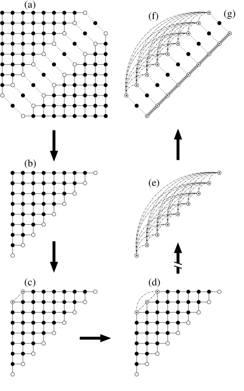
FIG. 1.: The decimation process: (a) The lattice is split into two parts. (b) Each half is then ‘decimated’ independently. (c,d) Sites ($\bullet$) and nearest-neighbor hops ($-$) in the original lattice are replaced successively by effective long-range hops ($-\cdot\cdot-$) between the effective sites ($\odot$). (e) This decimation continues until (f) the diagonal is reached. (g) Finally, the two halfs are recombined.

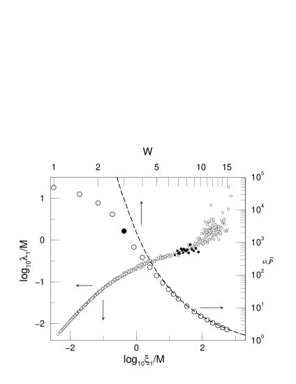
FIG. 2.: Small symbols (with left and bottom axis) denote the FSS curve used to compute the $\xi_{1}$ values. Large symbols (with right and top axis) indicate SP localisation lengths $\sqrt{2}\ \xi_{1}$ obtained by DM along the diagonal ($\circ$) and $\xi_{1}$ computed by TMM of quasi-1D strips (dashed line) after FSS. The filled symbols correspond to a disorder at which FSS appears to be unreliable.

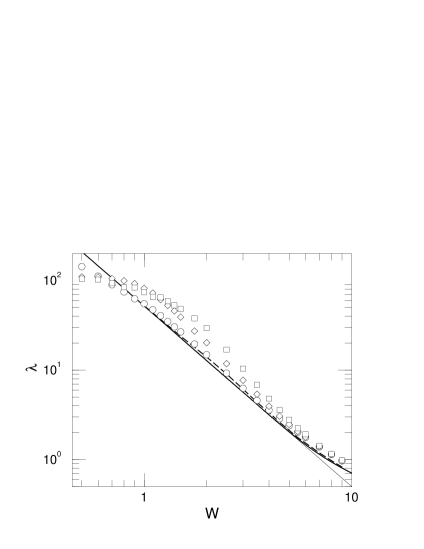
FIG. 3.: Two-particle localisation length $\lambda_{2}$ at energy $E=0$ for system size $M=201$ and interaction strength $U=0$ ($\bigcirc$), $U=0.2$ ($\Diamond$) and $U=1$ ($\Box$). The thick solid line represents 1D TMM data for SP localisation length $\lambda_{1}/2$, the dashed line is computed from the convolution of SP Green functions in Eq. (8). The thin line is the perturbative result $\lambda_{1}/2\approx 52/W^{2}$.

FIG. 4.: Enhancement $\lambda_{2}(U)/\lambda_{2}(0)$ for TIP as a function of interaction strength $U$ at $E=0$ for disorder $W=3$ ($+$), $W=4$ ($*$), and $W=5$ ($\times$) and $M=201$. The data are averaged over 100 samples. The thick (thin) lines indicate data for $U>0$ ($U<0$), full (open) circles denote the maximum for each disorder.

FIG. 5.: Enhancement $\lambda_{2}(U)/\lambda_{2}(0)$ for TIP as a function of interaction strength $U$ at $E=\pm 1$ for disorder $W=3$ ($+$), $W=4$ ($*$), and $W=5$ ($\times$) and $M=201$. The thick (thin) lines indicate data for $E=1$ ($E=-1$).

FIG. 6.: TIP localisation length $\lambda_{2}$ as a function of interaction strength $U$ at $W=4$ for $E=-2$ ($\triangleleft$), $E=-1$ ($\triangledown$), $E=0$ ($*$), $E=1$ ($\triangle$), and $E=2$ ($\triangleright$) and $M=201$. The thick (thin) lines indicate data for $E\geq 0$ ($E<0$).

FIG. 7.: Reduced TIP localisation lengths $\lambda_{2}/M$ for $U=0$ (left) and $U=1$ (right) for all disorders $W$ and system sizes $M$ obtained by averaging 1000 samples for each triple ($U,W,M$). Different letters indicate different disorders.

FIG. 8.: TIP localisation lengths $\lambda_{2}$ for $W=3$ (left) and $W=9$ (right) for $U=0,0.1,\ldots,1$ from bottom to top. We remark that we have taken the same set of random numbers for all $U$ to increase the numerical efficiency. This is probably the reason why for different $U$ the fluctuations in the dependence of $\lambda_{2}$ on $M$ are similar.

FIG. 9.: Finite-size scaling plot of the reduced TIP localisation lengths $\lambda_{2}/M$ for $U=0$ ($\bigcirc$), $U=0.2$ ($\Diamond$) and $U=1$ ($\Box$). The data for $U=0.2$ ($U=1$) have been divided by 2 (4) for clarity. Data corresponding to $W=1$ are indicated by filled symbols. The two curves at the bottom show the data for $U=0.2$ and $1$ and $W<2.5$, shifted downward by one order of magnitude for clarity, but with the data $W<1$ fitted with scaling parameters obtained from the fit in Fig. 11.

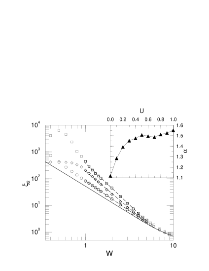
FIG. 10.: TIP localisation lengths $\xi_{2}$ after FSS for $U=0$ ($\bigcirc$), $U=0.2$ ($\Diamond$) and $U=1$ ($\Box$). The solid line represents 1D TMM data for SP localisation lengths $\lambda_{1}/2$, the dashed lines indicate power-law fits. Inset: Exponent $\alpha$ obtained by the fit of $\xi_{2}\propto W^{-2\alpha}$ to the data for $U=0,0.1,\ldots,1$.

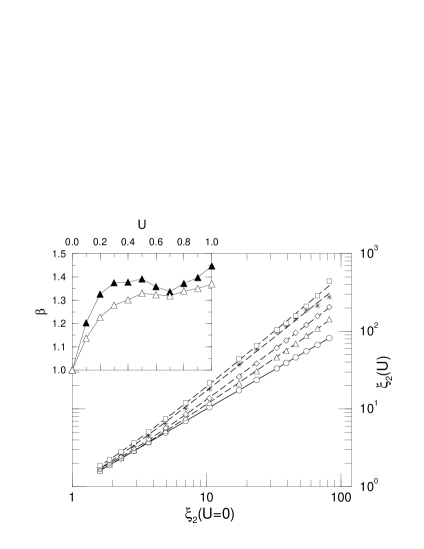
FIG. 11.: TIP localisation lengths $\xi_{2}(U)$ after FSS for $U=0$ ($\bigcirc$), $U=0.1$ ($\triangle$), $U=0.2$ ($\Diamond$), $U=0.5$ ($*$) and $U=1$ ($\Box$) plotted versus $\xi_{2}(0)$. The data are for $W\in[1,6]$. The dashed lines show fits according to Eq. (9), the solid line sets the reference for $U=0$. Inset: Exponent $\beta$ obtained by the fit of Eq. (9) to the data for $U=0,0.1,\ldots,1$. The open symbols correspond to the fit with $c=0$.

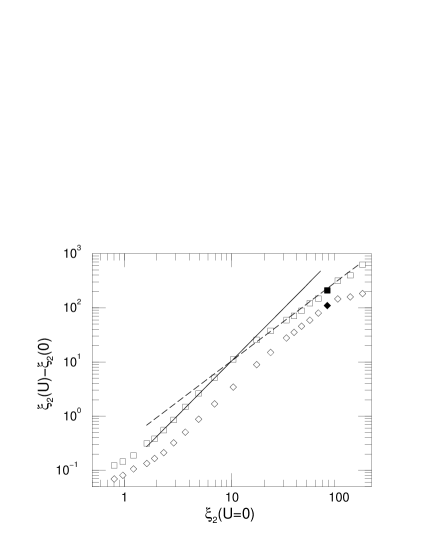
FIG. 12.: TIP localisation lengths $\xi_{2}$ plotted according to Eq. (10) for $U=0.2$ ($\Diamond$) and $U=1$ ($\Box$). The solid line indicates a slope $2$, the dashed line a slope $3/2$. The filled symbols correspond to $W=1$.

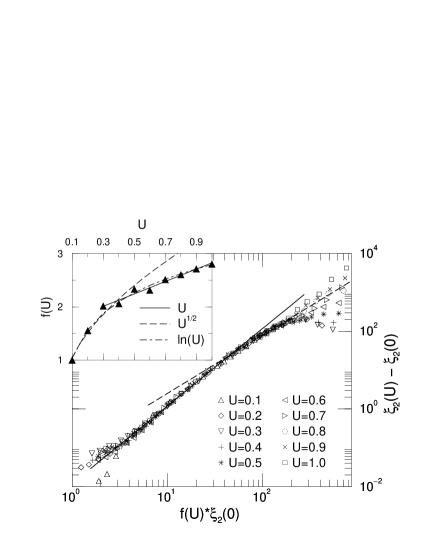
FIG. 13.: Scaling plot of Eq. (12) with TIP localisation lengths $\xi_{2}$ for all $U$ and $W\in[0.6,9]$. The solid line indicates a slope 2, the dashed line a slope 3/2. Inset: The values of $f(U)$ needed to make the data collapse onto the $U=0.1$ curve. Solid, dashed and dot-dashed lines are fits of $f(U)$ for $U\geq 0.3$, $U\leq 0.5$, and all $U$, respectively.

FIG. 14.: Enhancement $\lambda_{2}(U)/\lambda_{2}(0)$ for IEH as a function of interaction strength $U$ at $E=0$ for disorder $W=3$ ($+$), $W=4$ ($*$), and $W=5$ ($\times$) and $M=201$. The data are averaged over 100 samples. The thick (thin) lines indicate data for $U>0$ ($U<0$).

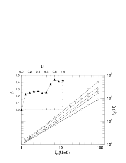
FIG. 15.: IEH localisation lengths $\xi_{2}(U)$ after FSS for $U=0$ ($\bigcirc$), $U=0.1$ ($\triangle$), $U=0.2$ ($\Diamond$), $U=0.5$ ($*$) and $U=1$ ($\Box$) plotted versus $\xi_{2}(0)$. The lines are fits as in Fig. 11. Inset: Exponent $\beta$ obtained by fitting Eq. (9) to the data for $U=0,0.1,\ldots,1$.

FIG. 16.: SP localisation lengths as in Fig. 2 for $U=0$ (– –, $\bigcirc$) and $\sqrt{2}\ \xi_{1}$ obtained by DM for $U=1$ with additional random ($\Box$) or constant ($\times$) potential energies along the diagonal.

- [1] see, e.g., P. A. Lee and T. V. Ramakrishnan, Rev. Mod. Phys. 57, 287 (1985) and D. Belitz and T. R. Kirkpatrick, Rev. Mod. Phys. 66, 261 (1994).
- [2] E. Abrahams, P. W. Anderson, D. C. Licciardello, and T. V. Ramakrishnan, Phys. Rev. Lett. 42, 673 (1979).
- [3] S. V. Kravchenko, D. Simonian, and M. P. Sarachik, Phys. Rev. Lett. 77, 4938 (1996).
- [4] D. L. Shepelyansky, Phys. Rev. Lett. 73, 2607 (1994); F. Borgonovi and D. L. Shepelyansky, Nonlinearity 8, 877 (1995); —, J. Phys. I France 6, 287 (1996).
- [5] D. L. Shepelyansky, Proc. Moriond Conf., Jan. 1996, cond-mat/9603086.
- [6] G. Czycholl, B. Kramer, and A. MacKinnon, Z. Phys. B 43, 5 (1981); J.-L. Pichard, J. Phys. C 19, 1519 (1986).
- [7] M. Kappus and F. Wegner, Z. Phys. B 45, 15 (1981);
- [8] Y. Imry, Europhys. Lett. 30, 405 (1995).
- [9] T. Giamarchi and H. J. Schulz, Phys. Rev. B 37, 325 (1988); C. L. Kane and M. P. A. Fisher, Phys. Rev. Lett. 68, 1220 (1992).
- [10] A. MacKinnon and B. Kramer, Z. Phys. B 53, 1 (1983).
- [11] K. Frahm, A. Müller-Groeling, J.-L. Pichard, and D. Weinmann, Europhys. Lett. 31, 169 (1995).
- [12] D. Brinkmann, J. E. Golub, S. W. Koch, P. Thomas, K. Maschke, I. Varga, preprint (1998).
- [13] D. Weinmann, A. Müller-Groeling, J.-L. Pichard, and K. Frahm, Phys. Rev. Lett. 75, 1598 (1995).
- [14] F. v. Oppen, T. Wettig, and J. Müller, Phys. Rev. Lett. 76, 491 (1996).
- [15] P. H. Song and D. Kim, Phys. Rev. B 56, 12217 (1997).
- [16] R. A. Römer and M. Schreiber, Phys. Rev. Lett. 78, 515 (1997); K. Frahm, A. Müller-Groeling, J.-L. Pichard, and D. Weinmann, Phys. Rev. Lett. 78, 4889 (1997); R. A. Römer and M. Schreiber, Phys. Rev. Lett. 78, 4890 (1997).
- [17] R. A. Römer and M. Schreiber, phys. stat. sol. (b) 205, 275 (1998).
- [18] O. Halfpap, A. MacKinnon, and B. Kramer, to be published in Sol. State. Comm., (1998); O. Halfpap, I. Kh. Zharekeshev, B. Kramer, and A. MacKinnon, preprint (1998).
- [19] C. J. Lambert, D. Weaire, phys. stat. sol. (b) 101, 591 (1980).
- [20] The values obtained here are defined as half the values of Refs. [11, 16, 17, 18].
- [21] T. Vojta, R. A. Römer, and M. Schreiber, preprint (1997, cond-mat/9702241).
- [22] I. V. Ponomarev and P. G. Silvestrov, Phys. Rev. B 56, 3742 (1997).
- [23] X. Waintal, D. Weinmann, and J.-L. Pichard, preprint (1998, cond-mat/9801134).
- [24] D. Weinmann and J.-L. Pichard, Phys. Rev. Lett. 77, 1556 (1996).
- [25] X. Waintal and J.-L. Pichard, preprint (1998, cond-mat/9706258).
- [26] J. E. Golub, private communication.