Diagonal Ladders: A New Class of Models for Strongly Coupled Electron Systems

Abstract

We introduce a class of models defined on ladders with a diagonal structure generated by $n_{p}$ plaquettes. The case $n_{p}=1$ corresponds to the necklace ladder and has remarkable properties which are studied using DMRG and recurrent variational ansatzes. The AF Heisenberg model on this ladder is equivalent to the alternating spin-1/spin-$\frac{1}{2}$ AFH chain which is known to have a ferrimagnetic ground state (GS). For doping 1/3 the GS is a fully doped (1,1) stripe with the holes located mostly along the principal diagonal while the minor diagonals are occupied by spin singlets. This state can be seen as a Mott insulator of localized Cooper pairs on the plaquettes. A physical picture of our results is provided by a $t_{p}-J_{p}-t_{d}$ model of plaquettes coupled diagonally with a hopping parameter $t_{d}$. In the limit $t_{d}\rightarrow\infty$ we recover the original $t-J$ model on the necklace ladder while for weak hopping parameter the model is easily solvable. The GS in the strong hopping regime is essentially an “on link” Gutzwiller projection of the weak hopping GS. We generalize the $t_{p}-J_{p}-t_{d}$ model to diagonal ladders with $n_{p}>1$ and the 2D square lattice. We use in our construction concepts familiar in Statistical Mechanics such as medial graphs and Bratelli diagrams.

]

I Introduction

Ladders provide a class of interesting theoretical models for studying the behavior of strongly correlated electron systems. Besides representing simplified models for actual materials, ladders offer a possible way of interpolating between 1 and 2 spatial dimensions with the hope that they will yield insights into the physics of 2D systems, such as the $CuO_{2}$ planes of the cuprates (for a review see [1]).

It has been found that ladders exhibit quite different behavior depending on whether the number of legs $n_{\ell}$ is even or odd. Antiferromagnetic spin ladders with $n_{\ell}$ odd are gapless with spin-spin correlation functions decaying algebraically, while even leg ladders are gapped with a finite spin correlation length. Upon doping, these two types of ladders also behave differently concerning the existence of pairing of holes or spin-charge separation. In the limit where the number of legs goes to infinity the spin gap of the even spin ladders vanishes exponentially fast, in agreement with the gapless nature of the 2D magnons [2]. On the other hand, the antiferromagnetic long range order (AFLRO) characteristic of the 2D antiferromagnetic Heisenberg (AFH) model can be more naturally attributed to the quasi long range order of the odd leg ladders. It thus seems that one has to combine different properties of the even and odd, doped and undoped ladders in order to arrive at a consistent picture of the 2D cuprates. Ladder systems are sufficiently interesting on their own to deserve detailed studies, in addition there are a variety of materials which contain weakly coupled arrays of ladders[3].

In this paper we study of a class of ladders characterized by a diagonal structure which provides an alternative to the aforementioned route to 2D. We shall call these objects diagonal ladders in order to distinguish them from the more familiar rectangular shaped ones. Diagonal ladders are labelled by an integer $n_{p}=1,2,\dots$ which gives the number of elementary plaquettes needed to generate the entire structure. The first member of this family, i.e. $n_{p}=1$, is also known as the necklace ladder and it consists of a collection of $N$ plaquettes joined along a common diagonal. In this paper we shall focus on the necklace ladder, although the other cases will also be briefly considered.

The original motivation of this work was to understand the fully doped stripes in the (1,1) direction that have been observed experimentally in materials like La_1-xSr_xNiO₄[4], in Hartree-Fock studies of $t-J$ and Hubbard models[5], and numerically in density matrix renormalization group[6] (DMRG) studies of the $t-J$ model [7]. The simplest possible toy model of this type of stripes is provided by a necklace ladder with a hole doping equal to 1/3. As we shall see this doping plays an important role in our work.

Lattices similar to the diagonal ladders, but with additional one-electron hopping terms along the major and minor diagonals of each plaquette, and with $J/t=0$, have been solved exactly for certain fillings[8, 9, 10]. Giesekus[10] has shown that for the corresponding version of the necklace ladder, in the case when all of the one-electron hopping terms are equal and the hole doping is set to $x=1/3$, the model has a short range RVB ground state, in which the static correlations exhibit an exponential decay and the dynamic correlation functions exhibit a gap in their spectral densities.

Let us also note in passing that diagonal ladders have recently appeared as constituent parts of some interesting materials like Sr_0.4Ca_13.6Cu₂₄O_41.84 known for its superconducting properties at high pressure [11]

The organization of the paper is as follows. In Section II we define the diagonal ladders from a geometrical viewpoint and compare them with the more familiar ladder structures. In Section III we study the AF Heisenberg model of the necklace ladder. In Section IV we study the $t-J$ model on the necklace ladder and show the conservation of the parity of the plaquettes. In Section V we present the ground state (GS) structure of a necklace $t-J$ ladder with 7 plaquettes, obtained with the DMRG and recurrent variational ansatz (RVA) methods. In Section VI we study in more detail the structure of the GS at doping 1/3. In Section VII we introduce a generalized $t-J$ model on an enlarged necklace ladder, called the $t_{p}-J_{p}-t_{d}$ model, and use it to give a physical picture of the results of Sections V and VI. In Section VIII we define the $t_{p}-J_{p}-t_{d}$ model on diagonal ladders with more than one plaquette per unit cell and on the 2D square lattice. In Section IX we state our conclusions. There are three appendices which give the technical details concerning the RVA calculations (Appendix A), the complete spectrum of the $t-J$ Hamiltonian on a plaquette (Appendix B) and a plaquette derivation of the equivalence between the spin 1 AKLT state of a chain and the dimer-RVB state of the 2-leg AFH ladder (Appendix C).

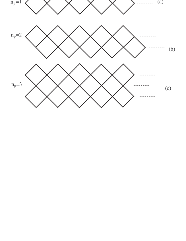
FIG. 1.: Examples of diagonal ladders with a number of plaquettes $n_{p}=1,2,3$ in the unit cell.

II Geometry of Diagonal Ladders

A diagonal ladder can be characterized by the number of plaquettes $n_{p}$ of the unit cell and the number $N$ of these cells. In Fig. 1 we show diagonal ladders with $n_{p}=1,2$ and 3. There are $n_{p}+2$ sites per unit cell. Assuming open boundary conditions the total number of sites is then given by $N_{s}=(n_{p}+2)N+n_{p}$.

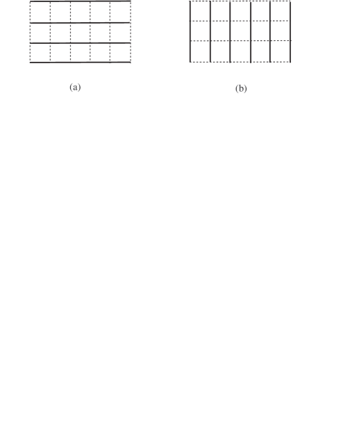
FIG. 2.: (a)Weak coupling (dashed lines) regime in rectangular ladders. (b)Strong couping (dashed lines) regime in rectangular ladders.

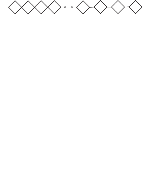
FIG. 3.: Plaquette construction (right) of a diagonal ladder (left).

Rectangular ladders can be seen either as a collections of legs coupled along the rungs or as collections of rungs coupled along the legs (see Fig. 2). This geometric feature is the basis of the weak coupling and strong coupling approaches to the various physical models defined on ladders. Thus for example the Heisenberg model on the $n_{\ell}$-leg ladder is usually defined with an exchange coupling constant $J_{\parallel}$ along the legs and an exchange coupling constant $J_{\perp}$ along the rungs. The weak and strong coupling limits correspond to the cases where $J_{\parallel}>>J_{\perp}$ and $J_{\parallel}<<J_{\perp}$ respectively.

On the other hand diagonal ladders do not admit such a simple construction. The most natural interpretation is to regard them as collections of plaquettes joined along their common diagonal (see Fig. 3). The trouble with this construction is that it does not preserve the number of sites! Indeed one has to fuse the points on the principal diagonal of the plaquettes before getting the actual necklace structure. We shall resolve this problem in Section VII on physical grounds.

III The spin necklace ladder

Let us begin by considering the AFH model on the necklace ladder of Fig. 1(a). The Hamiltonian of the model is simply,

$$H=J\;\sum_{<i,j>}{\bf{S}}_{i}\cdot{\bf{S}}_{j}$$ (1)

where $J$ is a positive exchange coupling constant and the sum runs over all links $<i,j>$ of the ladder. We shall label the sites of the $n^{\rm th}$ plaquette as in Fig. 4. The Hamiltonian (1) then becomes

$$H=J\sum_{n=1}^{N}\;\;({\bf{S}}_{1,n}+{\bf{S}}_{2,n})\cdot({\bf{S}}_{3,n}+{\bf{S}}_{3,n-1})$$ (2)

where ${\bf{S}}_{a,n}$ is a spin 1/2 operator acting at the $a=1,2,3$ position of the $n^{\rm th}$ plaquette. Eq.(2) implies that $H$ depends on the spins of the minor diagonals through their sum

$${\bf{S}}_{12,n}\equiv{\bf{S}}_{1,n}+{\bf{S}}_{2,n}$$ (3)

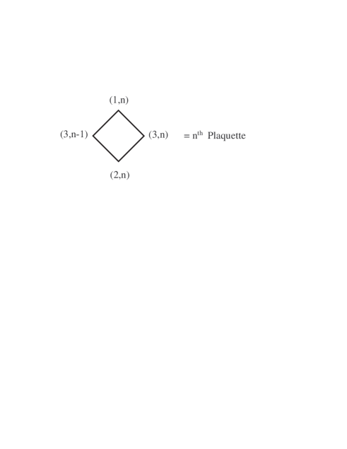
FIG. 4.: Diagonal coordinates for a single plaquette.

At this stage we are free to choose the spins of the $n^{\rm th}$ diagonal in the singlet ($S_{12,n}=0$) or triplet ( $S_{12,n}=1$) representations. In the latter case the Hamiltonian (2) becomes entirely equivalent to that of an alternating spin-1/spin-$\frac{1}{2}$ chain. Choosing a singlet on the minor diagonal of a given plaquette amounts to adding a spin zero impurity on the corresponding spin-1 site in the alternating chain, which therefore breaks into two disconnected pieces. The net result is that the spin necklace ladder in fact describes alternating spin-1/spin-$\frac{1}{2}$ chains with all possible sizes.

Fortunately, the alternating spin-1/spin-$\frac{1}{2}$ chain has been the subject of several studies concerning the ground state (GS), excitations, thermodynamic and magnetic properties [12, 13, 14]. The GS turns out to be ferrimagnetic with total spin given by $s_{G}=N/2$ where N is the number of unit cells of the chain. There are gapless excitations to states with spin $s_{G}-1$ and gapped excitations to states with spin $s_{G}+1$. In spite of the existence of gapless excitations, the chain has a finite correlation length $\xi\sim 1$, defined from the exponential decay of the spin-spin correlation function $<{\bf{S}}_{i}\cdot{\bf{S}}_{j}>$ after subtraction of the ferrimagnetic long range contribution. These results have been obtained by a combination of spin-wave, variational and DMRG techniques, with very satisfactory quantitative and qualitative agreement among them [12, 13].

FIG. 5.: DMRG results for the spin configuration for the G.S. of an undoped $8\times 3$ necklace ladder. The state has total spin $s_{G}=4$. The length of the arrow is proportional to $\langle S_{z}\rangle$, according the scale in the box.

We have confirmed some of these properties by applying DMRG and variational methods to the spin necklace ladder. In Fig. 5 we present a snapshot of the spin configurations of the GS of an $8\times 3$ ladder, obtained with the DMRG, which has total spin $s_{G}=4$. We find that the mean value of the spins near the center of the system are given by $<S^{z}_{1,n}>=<S^{z}_{2,n}>=0.396$ and $<S^{z}_{3,n}>=-0.292$ in agreement with the results of Ref. [12] namely $<S^{z}_{1,n}>=0.39624$ and $<S^{z}_{3,n}>=-0.29248$. Also using variational RVA methods we have found $<S^{z}_{1,n}>=0.4160$ and $<S^{z}_{3,n}>=-0.2893$.

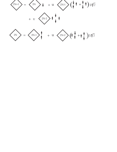
FIG. 6.: Diagrammatic representation of the Recurrent Relations generating the G.S. of an undoped necklace ladder using the variational RVA method (see Appendix A).

The existence of a very short correlation length suggests that the ferrimagnetic GS is an adiabatic deformation of the Néel state, which can be described by a short range variational state. References [12, 13] propose several variational matrix product states [15]. It is more convenient for our purposes to use the Recursive Variational Approach (RVA) of references [16, 17], in order to deal with doped and undoped cases on equal footing. The GS of a ladder of length $N$ is built up from the states with lengths $N-1,N-2$ and eventually $N-3$ if $N$ is odd. The GS thus generated is a $3^{\rm rd}$ order RVA state. In Fig. 6 we show a diagrammatic representation of the corresponding recurrence relations (we leave for Appendix A the technical details). The GS energy per site of the associated alternating chain that we obtain is given by $-0.7233J$, which is to be compared with the extrapolated DMRG results $-0.72704J$ or the spin-wave value $-0.718J$ of Pati et. al. [12].

IV The $t-J$ model on the necklace ladder

The Hamiltonian of the $t-J$ model is given by

$\displaystyle H_{t,J}={\cal P}_{G}\left(J\;\sum_{<i,j>}\;\;({{\bf S}}_{i}\cdot{{\bf{S}}_{j}}-\frac{1}{4}\;n_{i}\;n_{j})\right){\cal P}_{G}$

$$-{\cal P}_{G}\left(t\;\sum_{<i,j>,s}\;(c^{\dagger}_{i,s}\;c_{j,s}+h.c.)\right){\cal P}_{G}$$ (4)

where the $c_{i,s}\;(\;c^{\dagger}_{i,s}\;)$ is the electron destruction (creation) operator for site $i$ and spin $s$, $n_{i}$ is the occupation number operator, and ${\cal P}_{G}$ is the Gutzwiller projection operator which forbids doubly occupied sites. The density-density and kinetic terms in (4) can be written in a form similar to (2) for the exchange terms. This suggest that there will also be a “decoupling” of degrees of freedom associated with the transverse diagonals. The simplest way to see how this decoupling works is as follows.

For the necklace $t-J$ ladder, there is a parity plaquette conservation theorem[10]: the $t-J$ Hamiltonian on a necklace ladder commutes with every graded permutation operator $P_{n}$ associated with the minor diagonal of the $n^{\rm th}$ plaquette. Here the permutation operator $P_{n}(n=1,\dots,N)$ is defined by its action on the fermionic operators, which is trivial at all the sites except for those on the minor diagonal of the $n^{\rm th}$ plaquette where it acts as

$$P_{n}\;c_{(1,n),s}\;P_{n}^{\dagger}=\;c_{(2,n),s}$$ (5)

$$P_{n}\;c_{(2,n),s}\;P_{n}^{\dagger}=\;c_{(1,n),s}$$ (6)

Of course the spin and the density number operators at the sites $(1,n)$ and $(2,n)$ are also interchanged under the action of $P_{n}$. The above theorem is the statement that $P_{n}$ commutes with $H_{t,J}$, Eq.(4), for all $n$,

$$[H_{t,J},\;P_{n}]=\;0\;\;{\rm for}\;\;\;n=1,\dots,N$$ (7)

and can be easily proved. Eq.(7) is not special to the $t-J$ Hamiltonian, since any other lattice Hamiltonian having the permutation symmetry between the two sites on the minor diagonal of every plaquette would share this same property.

The immediate consequence of (7) is that we can simultaneously diagonalize the Hamiltonian $H_{t,J}$ and the whole collection of permutations operators $P_{n}$, whose possible eigenvalues are given by $\epsilon_{n}=\pm 1$. The latter fact is a consequence of the Eq.

$$P_{n}^{2}=1$$ (8)

Letting $\epsilon_{n}$ denote the parity of the $n^{\rm th}$ plaquette, the 9 possible states associated with the minor diagonal of a plaquette can be classified according to their parity, i.e. $\epsilon_{n}=1$ for even parity states and $\epsilon_{n}=-1$ for odd-parity states (see Table 1).

	State	$\epsilon$
2 holes	$|0\rangle$	1
bonding	$(c^{\dagger}_{1,s}+c^{\dagger}_{2,s})|0\rangle$	1
singlet	$\Delta^{\dagger}_{1,2}|0\rangle$	1
antibonding	$(c^{\dagger}_{1,s}-c^{\dagger}_{2,s})|0\rangle$	$-1$
triplet	$(c_{1,s}^{\dagger}c_{2,s^{\prime}}^{\dagger}+s\leftrightarrow s^{\prime})|0\rangle$	$-1$

Table 1. Classification of the states of the minor diagonal of a plaquette according to their parity. $\Delta_{1,2}^{\dagger}=\left(c_{1,\uparrow}^{\dagger}c_{2,\downarrow}^{\dagger}+c_{2,\uparrow}^{\dagger}c_{1,\downarrow}^{\dagger}\right)/\sqrt{2}$ is the pair field operator.

The Hilbert space ${\cal H}_{\rm necklace}$ of the $t-J$ model can be split into a direct sum of subspaces ${\cal H}_{\bf\epsilon}$ classified by the parity of their plaquettes, ${\bf\epsilon}=\{\epsilon_{n}\}_{n=1}^{N}$, namely

$${\cal H}_{\rm necklace}=\oplus_{{\bf\epsilon}}\;{\cal H}_{\bf\epsilon}$$ (9)

Every subspace ${\cal H}_{\bf\epsilon}$ is left invariant under the action of the $t-J$ Hamiltonian (4) which can therefore be projected into an “effective” Hamiltonian $H_{t,J}(\epsilon)$. In the previous section we have already seen an example of this type of decoupling phenomena. Indeed the alternating spin-1/spin-$\frac{1}{2}$ chain corresponds precisely to the case where all the plaquettes are odd and there are no holes. If holes are allowed then one has to consider, in addition to the triplets, the antibonding states on the odd plaquettes. Hence there are a total of 5 states at each site of the “effective” alternating chain associated with the minor diagonal of the odd plaquettes.

On the other hand, if the parity of the plaquette is even, then the corresponding site in the chain has 4 possible states which can be put into one-to-one correspondence with those of a Hubbard model as follows,

$$\begin{array}[]{rcl}{\rm Even}\;{\rm diagonal}&\longleftrightarrow&{\rm Hubbard}\;{\rm site}\\ {\rm empty(2\;holes)}&\longleftrightarrow&{\rm empty(1\;hole)}\\ {\rm bonding}\;{\rm states}\;(\uparrow,\downarrow)&\longleftrightarrow&{\rm single}\;{\rm occupied}\;{\rm state}\;(\uparrow,\downarrow)\\ {\rm singlet}\;{\rm state}&\longleftrightarrow&{\rm doubly}\;{\rm occupied}\;{\rm state}\\ \end{array}$$ (10)

In this case the Hamiltonian of the model is a $t-J$ Hamiltonian with hopping parameter equal to $\sqrt{2}t$ and with the same exchange and density-density couplings. There is no Hubbard $U$ term.

In summary, theorem (7) implies that the necklace ladder is in fact equivalent to a huge collection of alternating chains models where half of the sites are $t-J$ like while the other half may be either spin 1 or spin-$\frac{1}{2}$ antibonding states for odd parity, or Hubbard like, for even parity.

It is beyond the scope of the present paper to study such an amazing variety of chain models disguised in the innocent looking necklace ladder. Instead, a more reasonable strategy is to ask for the values of the total spin $S$ and parity $\epsilon$ which give the absolute minimum of the GS energy, keeping fixed the values of the number of plaquettes $N$, the number of holes $h$ and the ratio $J/t$, i.e.

$$E_{0}(N,h,S_{{\rm min}},{\bf\epsilon}_{\rm min},J/t)\leq E_{0}(N,h,S,{\bf\epsilon},J/t),\;\;\;\forall S,{\bf\epsilon},$$ (11)

Even this question is not easy to answer with full generality. However we shall study a few cases which suggests a general pattern for the behavior of the spin and parity as functions of doping.

V DMRG and RVA results on the necklace ladder

We shall concentrate on the case of a necklace ladder with 7 plaquettes and open BCs, which will allow us to present in a simple manner the basic features of the GS for various spins ($S$) and dopings ($h$). The values of the coupling constants are fixed to $t=1$ and $J=0.35$.

In Table 2 we show, for several pairs $(h,S)$ the parities of the plaquettes, the total GS energy computed with the DMRG and the RVA methods. This table also lists the label of the corresponding figures showing DMRG results for the hole and spin densities of the corresponding state.

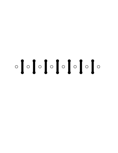
FIG. 7.: Pictorical representation of the most probable state for doped $x=1/3$ necklace ladder of dimension $8\times 8$. Blank circles denote holes and vertical solid lines represent valence bond states (Case (8,0)).

The RVA results have been derived from an inhomogeneous recurrence variational ansatz (see Appendix A). As in the latter cases we start from a state, hereafter called “classical”, which is considered to be the most important configuration present in the actual GS. Next we include the local quantum fluctuations around the classical state.

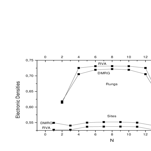
FIG. 8.: Electronic densities for a necklace ladder as depicted in Fig. 7. It corresponds to 7 plaquettes and 8 holes (doping $x=1/3$). Below are shown the DMRG and RVA values for the sites in the main diagonal, while above are shown the values on the rungs corresponding to subdiagonals.

This is done for a whole set of “classical” states having the same number of plaquettes, holes and $z$-component of spin. As discussed in the appendix, the classification of the “classical” states is achieved by means of paths in a Bratelli diagram generated by folding and repeating the Dynkin diagram of the exceptional group Lie $E_{6}$. The six points of $E_{6}$ are in one-to-one correspondence with 6 different states on the necklace ladder, while the links of $E_{6}$ are nearest neighbor constraints derived on the basis of the DMRG results in the region $0\leq x\leq 1/3$. The Bratelli construction gives us a systematic way to explore the GS manifold in the underdoped region $x\leq 1/3$. The overdoped region has to be studied with delocalized RVA states as discussed in references [16, 17].

h	S	($\epsilon_{1},\dots,\epsilon_{7})$	Figure	$E^{\rm DMRG}_{0}$	$E^{\rm RVA}_{0}$
8	0	$(+++++++)$	7 and 8	-16.554153	-16.33996
8	1	$(+++-+++)$	9	-16.284855	-16.00358
7	1/2	$(++++++-)$	10	-15.489511	-15.18141
6	0	$(-+++++-)$	11	-14.424805	-14.02286
6	1	$(-+++++-)$	12	-14.424798	-14.02286
9	1/2	$(+++++++)$	13	-16.746112	-
10	0	$(+++++++)$	14	-16.927899	-
10	1	$(+++++++)$	15	-16.718476	-

Table 2. DMRG and RVA total energies for a 7-plaquette necklace ladder with $h$ holes and total spin $S_{z}$. The string of epsilons is the pattern of parities in the subdiagonals (rungs).

Let us comment on the DMRG results shown in the figures.

• Case (8,0): This is the most interesting case and it corresponds to one hole per site along the principal diagonal. In the infinite length limit this state has doping $x=1/3$. For this reason we shall hereafter call this state the $x=1/3$ state. Figure 7 shows the most probable configuration which occurs when the holes occupy the principal diagonal of the ladder and the spins form perfect singlets along the minor diagonals. The latter fact implies that all the plaquettes are even (see Table 1). Figure 8 shows the electronic density along the ladder computed with the DMRG and the RVA.

  

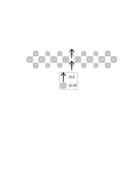
  FIG. 9.: Results using DMRG showing the necklace state with 8 holes and spin $S_{z}=1$. The diameter of the circles are proportional to the hole density, and the length of the arrows are porportional to $\langle S_{z}\rangle$, accoring to the scale in the box.

• Case (8,1): (See Fig.9) The spin excitation of the $x=1/3$ state is given by a spin 1 magnon strongly localized on an odd parity plaquette located at the center of the ladder. The other plaquettes remain even and spinless. The value of the spin gap is given by $\Delta_{s}=0.27$ (DMRG) and 0.32 (RVA).

  

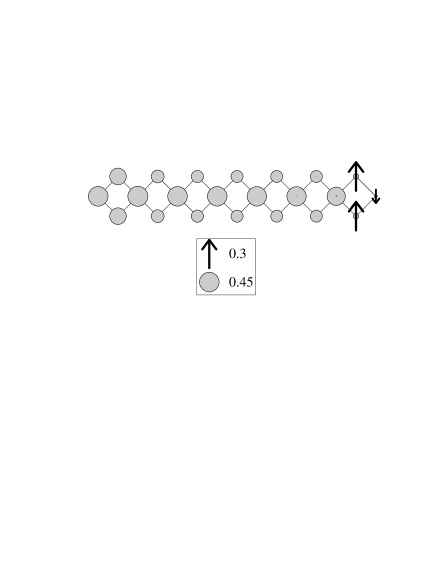
  FIG. 10.: DMRG results for the hole and spin densities of the necklace state with 7 holes and spin $S_{z}=1/2$.

• Case (7,1/2):(See Fig.10) This case is obtained by doping the $x=1/3$ state with an electron. The additional electron goes into either of the boundary plaquettes. The corresponding plaquette changes its parity to $-1$.

• Cases (6,0) and (6,1): (See Figs. 11-12) The state $x=1/3$ is now doped with two electrons, which go to the boundary plaquettes which change their parity. There seems to be a small effective coupling between the two spin 1/2 at the ends of the ladder, which lead to a breaking of the degeneracy between the triplet and the singlet. This is reminiscent of the effective spin 1/2 at the ends of the Haldane and AKLT open spin chains [18]. There also exists a weak effective coupling that breaks the four fold degeneracy of the open chains.

  

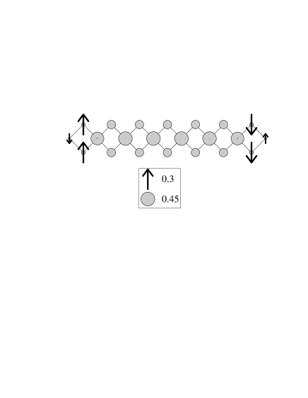
  FIG. 11.: Results from DMRG showing the necklace state with 6 holes and spin $S_{z}=0$.

  

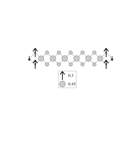
  FIG. 12.: Results from DMRG showing the necklace state with 6 holes and spin $S_{z}=1$.

• Case (9,1/2): (See Fig.13) The $x=1/3$ state is doped with one hole. The parity of the plaquettes remain unchanged and the extra spin 1/2 delocalizes along the whole system perhaps with some SDW component. The differences between this hole doped case and the electron doped case (7,1/2) are quite striking.

• Case (10,0) (See Fig.14) This state looks very much the same as the $x=1/3$ but just with more holes.

• Case (10,1) (See Fig.15) Same pattern as in the (9,1/2) case with the spin delocalized over the whole system.

In summary the DMRG results clearly suggest the existence of two distinct regimes corresponding to dopings $0\leq x<1/3$ and $x\geq 1/3$. In the overdoped regime the plaquettes are always even while in the underdoped regime they can be even or odd. Phase separation into even and odd plaquettes may also be possible. Our results at this moment are ambiguous and further numerical work is required. The most important result is the peculiar structure of the $x=1/3$ state, which we shall study further in the next two sections.

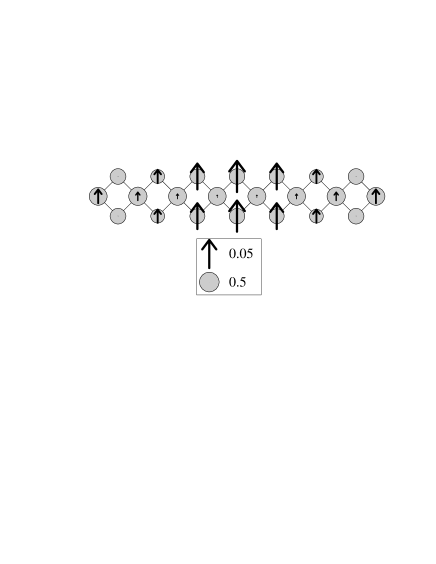
FIG. 13.: Results from DMRG showing the necklace state with 9 holes and spin $S_{z}=1/2$.

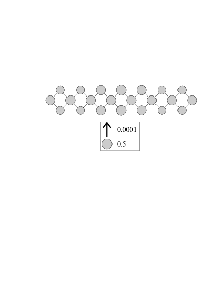
FIG. 14.: Results from DMRG showing the necklace state with 10 holes and spin $S_{z}=0$.

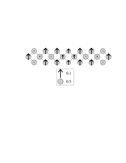
FIG. 15.: Results from DMRG showing the necklace state with 10 holes and spin $S_{z}=1$.

VI The $x=1/3$ state of the necklace ladder

The most important configuration contained in the $x=1/3$ state has spin singlets along the diagonal. This is consistent with and helps explain the $\pi$ phase shift in the (1,1) domain walls observed numerically with DMRG[7] and Hartree-Fock[5] calculations in large lattices and experimentally in some nickelates compounds.

On the other hand the $x=1/3$ state is a kind of 1D generalization of the GS of 2 holes and 2 electrons on the $2\times 2$ cluster discussed in reference [19], in connection with the binding of holes in the 2-leg and higher-leg ladders. One can also use this local structure to build up a variational state of the 2-leg ladder valid for any doping[17].

The GS of two holes in a plaquette is the localized Cooper pair depicted in Fig. 16 and can be generated by the pair field operators acting on the vacuum as,

$$|{\rm Cooper}\;{\rm Pair}>=$$ (12)

$$\left(A(\Delta_{1,3}^{\dagger}+\Delta_{1,4}^{\dagger}+\Delta_{2,3}^{\dagger}+\Delta_{2,4}^{\dagger})+(\Delta_{1,2}^{\dagger}+\Delta_{3,4}^{\dagger})\right)|0\rangle$$ (13)

where $A$ is given by

$$A=\frac{1}{[2+(J/4t)^{2}]^{1/2}-J/4t}$$ (14)

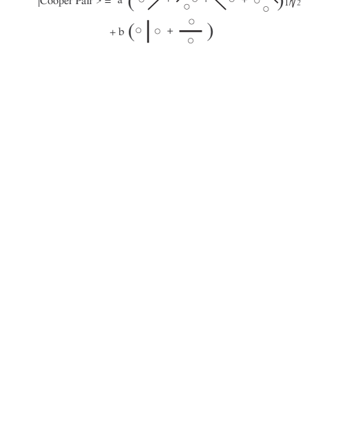
FIG. 16.: A pictorical representation of a localized Cooper pair on a plaquette. The parameter $A$ in (12) is $A=a/\sqrt{2},b=1$.

If $J/t<2$, then $A<1$ which means that a diagonal bond is more probable that a non-diagonal one. This feature is also observed in the $x=1/3$ state where the most probable bonds are those that line up along the transverse diagonals of the ladder ( Fig. 7). Taking into account this state together with some important local fluctuations around it lead us to propose an RVA state with $x=1/3$, which is defined by the recursion relations depicted in Fig. 17 (see Appendix A for details). The RVA state corresponding to $N=1$ plaquette coincides precisely with state (12) identifying $A=a/\sqrt{2},b=1$ (See Fig.16). For ladders with more than one plaquette ($N>1$) the symmetry of the diagonals disappear and $b\neq 1$ in general. In this case we have two independent variational parameters $a$ and $b$. In Fig. 18 we give the energy per plaquette and the values of $a$ and $b$ as functions of the number of plaquettes of the necklace ladder obtained by minimization of the energy of the RVA state. We observe that both $a$ and $b$ become less than one in agreement with the DMRG results. All these results are quite satisfactory but still they do not give us a transparent physical picture of the $x=1/3$ state. This will be done in the next section.

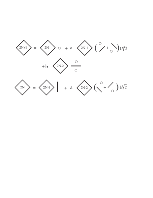
FIG. 17.: A pictorical representation of the Recurrence Relations employed with the RVA method (See Appendix A) to construct variational G.S. states for the doped $x=1/3$ necklace ladder. The diagonal squares represent bulk states of a given length. Small circles represent holes and solid lines valence bonds.

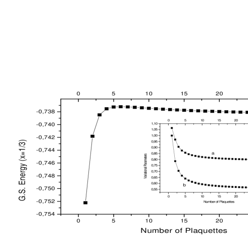
FIG. 18.: Ground state energy per site as function of the number of plaquettes for a doped $x=1/3$ necklace ladder. It is obtained using the RVA method (See Appendix A). Here $a$ and $b$ denote the variational parameters and it is shown how they get stabilized towards their thermodynamic values as the length of the ladder increases.

VII The plaquette picture of the necklace ladder: the $t_{p}-J_{p}-t_{d}$ model

An interesting property of the rectangular ladders is that the strong coupling picture of the GS and excited states is generally valid also in the intermediate and weak coupling regimes. Thus, for example, the spin gap of the 2-leg spin ladder can be seen in the strong coupling limit as the energy cost for breaking a bond along the rungs.

In Section II we suggested that diagonal ladders could be thought of as collections of coupled plaquettes (Fig. 3). The trouble is that in doing so one actually needs more sites than those available in the original lattice. Indeed the necklace ladder ${\cal L}^{D}$ with $N$ plaquettes has $3N$ sites for $N$ large while the extended or decorated ladder ${\cal L}^{P}$ shown on the right hand side of Fig. 3 has $4N$.

The solution of this problem is achieved on physical grounds by defining on the lattice ${\cal L}^{P}$ an extended $t-J$ Hamiltonian which, in a certain strong coupling limit, becomes equivalent to the standard $t-J$ Hamiltonian on ${\cal L}^{D}$. The extended Hamiltonian can also be studied in the limit where the plaquettes are weakly coupled. As we shall see, the latter limit provides a useful physical picture of the properties of the necklace ladder for $x=1/3$ and other dopings as well.

A The $t_{p}-J_{p}-t_{d}$ model

We shall define on the lattice ${\cal L}^{P}$ an extended $t-J$ model by the following Hamiltonian,

$${H}_{pd}= H_{p}+H_{d}$$ (15)

$$H_{p}= \sum_{n}\,\,h_{n}(t_{p},J_{p})$$ (16)

$$H_{d}= \sum_{n}\,\,h_{n,n+1}(t_{d})$$ (17)

where $h_{n}(t_{p},J_{p})$ is a standard $t_{p}-J_{p}$ Hamiltonian involving only the 4 sites of the plaquette labelled by $n$. Of course $h_{n}$ and $h_{m}$ commute for $n\neq m$. On the other hand, $h_{n,n+1}(t_{d})$ is a hopping Hamiltonian associated with the link that connects the two nearest neighbor plaquettes $n$ and $n+1$. Denoting by $L$ and $R$ the corresponding sites on the different plaquettes joined by the link $<L,R>$ then $h_{n,n+1}$ is given by the link Hamiltonian defined as

$$h_{<L,R>}=t_{d}({c}^{\dagger}_{L,s}-{c}_{R,s}^{\dagger})\left({c}_{L,s}-{c}_{R,s}\right)$$ (18)

B Strong hopping limit of the $t_{p}-J_{p}-t_{d}$ model

We want to prove that in the strong hopping limit, where $t_{d}\rightarrow\infty$, the $t_{p}-J_{p}-t_{d}$ model becomes equivalent to the $t-J$ model on the necklace ladder ${\cal L}^{D}$.

In this limit we first diagonalize $H_{d}$ looking for the low energy modes of the plaquettes. We then define a renormalization group (RG) operator $T$, that leads to a renormalization of operators in the extended lattice model into operators that act on the necklace lattice. In particular the $H_{pd}$ Hamiltonian is truncated to an effective Hamiltonian which is equivalent to the original necklace Hamiltonian. The truncation operation is given by the Eq. (for a review of the Real Space RG method see [20])

$$H_{\rm eff}=T\,{H}_{pd}\,T^{\dagger}$$ (19)

The Hamiltonian $h_{n,n+1}(t_{d})$ acts in a Hilbert space of dimension $3\times 3=9$. It has two eigenvalues $E=0$ and $2t_{d}$, with degeneracies 3 and 6 respectively. The zero eigenvalue corresponds to the states with two holes and the bonding state with up and down spins. In the limit $t_{d}>>t_{p},J_{p}$ one retains only the latter 3 degrees of freedom which can be thought of as renormalized hole and spin up and spin down electron states, respectively. The truncation operator $T$, that maps the Hilbert space ${\cal H}_{{\cal L}^{P}}$ into the effective Hilbert space ${\cal H}_{{\cal L}^{D}}$ is, given by

$$\begin{array}[]{rcl}T:{\cal H}_{{\cal L}^{P}}&\rightarrow&{\cal H}_{{\cal L}^{D}}\\ |\bullet,\bullet\rangle&\rightarrow&0\\ |\bullet,\circ\rangle&\rightarrow&\frac{1}{\sqrt{2}}|\ast\rangle\\ |\circ,\bullet\rangle&\rightarrow&\frac{1}{\sqrt{2}}|\ast\rangle\\ |\circ,\circ\rangle&\rightarrow&|o\rangle\end{array}$$ (20)

where $\bullet$ and $\circ$ stand for one electron, with spin up or down, and one hole respectively living on a given link of ${\cal L}^{P}$, while $\ast$ and $o$ are the effective electron and holes living on the corresponding site of ${\cal L}^{D}$ obtained by contracting the previous link to a site. The hermitean operator $T^{\dagger}$ acts as follows,

$$\begin{array}[]{rcl}T^{\dagger}:{\cal H}_{{\cal L}^{D}}&{\rightarrow}&{\cal H}_{{\cal L}^{P}}\\ |\ast\rangle&\rightarrow&\frac{1}{\sqrt{2}}\left(|\bullet,\circ\rangle+|\circ,\bullet\rangle\right)\\ |o\rangle&\rightarrow&|\circ,\circ\rangle\end{array}$$ (21)

Eq.(21) means that an electron state $|\ast\rangle$ of ${\cal L}^{D}$ becomes the bonding state in the enlarged Hilbert space ${\cal H}_{{\cal L}^{P}}$. The RG operators $T$ and $T^{\dagger}$ defined above satisfy the following Eqs.[20]

$$T\;T^{\dagger}={\bf 1},\;\;\;\;T^{\dagger}\;T=P_{G}^{(\ell)}$$ (22)

where $P_{G}^{(\ell)}$ is a Gutzwiller operator which now acts on links rather than on sites as follows,

$$\begin{array}[]{rcl}P^{(\ell)}_{G}:{\cal H}_{{\cal L}^{P}}&\rightarrow&{\cal H}_{{\cal L}^{P}}\\ |\bullet,\bullet\rangle&\rightarrow&0\\ |\bullet,\circ\rangle&\rightarrow&\frac{1}{\sqrt{2}}\left(|\bullet,\circ\rangle+|\circ,\bullet\rangle\right)\\ |\circ,\bullet\rangle&\rightarrow&\frac{1}{\sqrt{2}}\left(|\bullet,\circ\rangle+|\circ,\bullet\rangle\right)\\ |\circ,\circ\rangle&\rightarrow&|\circ,\circ\rangle\end{array}$$ (23)

Using the above definitions we can easily obtain the renormalization of the different operators acting in ${\cal L}^{P}$,

$$\begin{array}[]{rl}T\;{c}_{L,s}\;T^{\dagger}=T\;{c}_{R,s}\;T^{\dagger}=&\frac{1}{\sqrt{2}}c_{M,s}\\ T\;{{\bf S}}_{L}\;T^{\dagger}=T\;{{\bf S}}_{R}\;T^{\dagger}=&\frac{1}{2}{\bf S}_{M}\\ T\;{n}_{L}\;T^{\dagger}=T\;{n}_{R}\;T^{\dagger}=&\frac{1}{2}n_{M}\ .\end{array}$$ (24)

Here ${c}_{i,s},{{\bf S}}_{i},{n}_{i}$ are the fermion, spin and number operators acting at the edges of the link $<L,R>$ for $i=L,R$ while for $i=M$ they act at the effective “middle” point of the link (i.e. $<L,R>\rightarrow M$). Of course, the operators and states that are not on the principal diagonal of both ${\cal L}^{P}$ and ${\cal L}^{D}$ are not affected by the renormalization procedure.

Using Eqs (19) and (24) we can immediately find that the renormalized effective Hamiltonian is given by the $t-J$ Hamiltonian (4), i.e.

$$H_{\rm eff}\equiv T\;{H}_{pd}\;T^{\dagger}=T\;H_{p}(t_{p},J_{p})\;T^{\dagger}=H_{t,J}$$ (25)

with the following values for the coupling constants,

$$t=\frac{1}{\sqrt{2}}\;t_{p},\;\;\;\;\;J=\frac{1}{{2}}\;J_{p},\;\;\;({\rm necklace}\;\;{\rm ladder})$$ (26)

In the derivation of (26) we are assuming periodic boundary conditions, along the principal diagonal of the necklace ladder.

The strong hopping limit studied above is reminiscent of the strong coupling limit of the Hubbard model which leads to the t-J model plus some extra three-site terms which are usually ignored. In the latter case the strong Coulomb repulsion forces the Gutzwiller on-site constraint. Our case is a “dual version” of this mechanism, in the sense that the coupling constant involved is a hopping parameter, and that the Gutzwiller constraint arises from a link rather than from a site constraint. In the case of the $t_{p}-J_{p}-t_{d}$ model one does not have to do perturbation theory in order to produce the exchange term in the effective Hamiltonian since it is already contained in the plaquette Hamiltonian. Perturbation theory would produce terms of the order $1/t_{d}$, but they vanish at $t_{d}=\infty$. The construction we have performed in this section can in principle be generalized to the Hubbard model[21].

The analogy between the Hubbard and the $t_{p}-J_{p}-t_{d}$ model suggests that we may learn something about the strong hopping limit by studying the weak hopping one. This is certainly true if there are no phase transitions between the two regimes.

C Weak Hopping Limit of the $t_{p}-J_{p}-t_{d}$ model

In the weak hopping regime, i.e. $t_{d}<<t_{p},J_{p}$, we first diagonalize the plaquette Hamiltonian $H_{p}$ and treat $H_{d}$ as a perturbation. The energy levels of $H_{p}$ are given, to lowest order in perturbation theory, as tensor products of the eigenstates of every plaquette. There will be in general a huge degeneracy, which will be broken by the effective Hamiltonian derived from $H_{d}$ using perturbation theory. Before going further into the study of the plaquette Hamiltonian we have to consider the relationship between the filling factors of the states belonging to lattices with different number of sites.

Let us consider a state in ${\cal L}^{D}$ with $N_{h}$ holes and $N_{e}$ electrons. Applying the operator $T^{\dagger}$, this state is transformed to a state in ${\cal L}^{P}$ with $N^{(p)}_{h}$ holes and $N^{(p)}_{e}$ electrons given by,

$$N_{h}^{(p)}=\frac{4}{3}N_{h}+\frac{1}{3}N_{e},\;\;{N_{e}}^{(p)}=N_{e}$$ (27)

These equations reflect the fact one gets an extra hole upon going to the enlarged lattice. Eqs.(27) imply the following relations between the doping factors $x=N_{h}/(N_{h}+N_{e})$ and ${x}_{p}={N_{h}}^{(p)}/({N_{h}}^{(p)}+{N_{e}}^{(p)})$,

$$\;x=\frac{1}{3}(4{x}_{p}-1),\;\;\;{x}_{p}=\frac{1}{4}(1+3\;x)\;\;\;$$ (28)

From (28) we get the following correspondences

$$x=0\longleftrightarrow{x}_{p}=1/4$$ (29)

$$x=1/3\longleftrightarrow{x}_{p}=1/2$$ (30)

which we shall discuss in detail below.

Weak hopping picture of the $x=1/3$ state

Eq.(29) implies that the 1/3 doped state of the necklace ladder is transformed to a state with two holes and two electrons per plaquette in the expanded necklace lattice. We show in appendix B that the lowest GS for this filling is given by the coherent superposition of Cooper pairs localized on the plaquettes, i.e.

$$|{x}_{p}=1/2,t_{d}=0>=\prod_{n=1}^{N}\;\;|{\rm Cooper}\;{\rm pair}>_{n}$$ (31)

where $|{\rm Cooper}\;{\rm pair}>_{n}$ is the state given in Eq..(12) with the parameters $a$ and $b$ given by Eq.(14) for the values of $t_{p},J_{p}$.

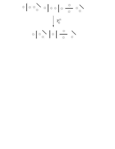
FIG. 19.: Ground state for a doped $x=1/3$ necklace ladder (down) obtained as the projection of a $x_{p}=1/2$ doped state in the decorated (dual) diagonal ladder (above).

Turning $t_{d}$ on, the state (31) will be perturbed mainly along the principal diagonal. The doubly occupied and antibonding links will become high energy states while the bonding and empty links will remain low in energy. In the limit when $t_{d}$ becomes infinite we expect the GS (31) to evolve continuously into the $x=1/3$ GS of the necklace. This suggest that the $x=1/3$ state of the necklace ladder can be described as a Gutzwiller projected state, i.e.

$$|x=1/3>\sim T\;{\cal P}_{G}^{(\ell)}\;|{x}_{p}=1/2,t_{d}=0>$$ (32)

where we first project out the doubly occupied and antibonding states on the links on the principal diagonal of the expanded ladder and then project the resulting state into the Hilbert space of the necklace ladder. Some diagrammatics (Fig. 19) shows that the state (32) is basically the same as the $x=1/3$ RVA state constructed in Section VI. This leads us to the conclusion that the $x=1/3$ GS of the necklace ladder can be seen as the Gutzwiller projection of Cooper pairs localized on the plaquettes. In this case the Cooper pairs are locked in a Mott insulating phase and there is an exponential decay of the pair field.

Weak hopping picture of the $x=0$ state

The GS of a plaquette with 1 hole and 3 electrons for $J_{p}/t_{p}=0.5$ has spin 1/2 and it belongs to the 2-dimensional irrep labelled by $E$ of the symmetry group $D_{4}$ (see Appendix B). These two states differ in their parity along the minor diagonal which can be even or odd. Both states can be thought of as bound states of a Cooper pair and one electron ( see Fig. 20). The four fold degeneracy on every plaquette is broken by $t_{d}$. The odd parity plaquettes are lower in energy than the even ones and the effective model is given by a ferromagnetic spin 1/2 chain,

$$H_{\rm eff}=J_{\rm eff}\;\;\sum_{n}\;{\bf S}_{n}^{\rm eff}\cdot{\bf S}_{n+1}^{\rm eff}$$ (33)

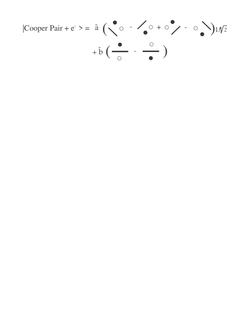
FIG. 20.: A pictorical representation of a bound state formed by a Cooper pair and one electron. Small blank circles represent holes, black circles represent electrons and solid lines are valence bonds. Here $\bar{a}$, $\bar{b}$ are relative amplitudes taken as variational parameters.

Here ${\bf S}_{n}^{\rm eff}$ is the overall spin 1/2 operator of the odd plaquette and $J_{\rm eff}\sim-t_{d}^{2}$ is a ferromagnetic exchange coupling constant.

Following a reasoning similar to that for the case $x=1/3$ we conjecture that the $x=0$ state can be represented as the following Gutzwiller projected state,

$$|x=0>\sim T\;{\cal P}_{G}^{(\ell)}\;|{x}_{p}=1/4,\epsilon_{n}=-1,t_{d}=0>$$ (34)

whose structure is indeed very similar to the ferrimagnetic RVA state proposed in Section III. See Fig. 21 for a plaquette construction of the Néel state of the necklace ladder starting from the ${x}_{p}=1/4,\;\;\epsilon_{n}=-1$ state. The gapless excitations of the ferrimagnetic $x=0$ GS correspond, in the weak coupling picture, to the magnons of the ferromagnetic chain (34), while the gapped excitations correspond to an excitation of the plaquette to a state with spin 3/2.

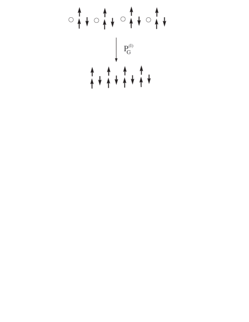
FIG. 21.: A Neel-like ground state (down) for an undoped $x=0$ necklace ladder obtained as the projection (above) of a doped state in the decorated (dual) diagonal ladder.

In summary we have been able to obtain a satisfactory picture of both the $x=0$ and 1/3 states in the weak coupling limit of the extended $t-J$ model, which leads us to conclude that for these dopings there are no phase transition between the weak and strong coupling regimes. Other dopings involve the competition of the two elementary plaquettes states used above and will be considered elsewhere.

VIII From 1D to 2D through diagonal ladders

The necklace ladder represents the first step in the diagonal route to the 2D square lattice. In this section we shall push forward this viewpoint trying to see how much one can expect from it. This will lead us to ask questions whose solution we do not yet know. In this sense some of the material presented below is conjectural.

Let us first start with a short excursion into graph theory.

A The plaquette construction and medial graphs

The plaquette construction of the necklace ladder is related to the so called medial graphs used in the coloring problem or in Statistical Mechanics [23]. Before we show this connection we need to generalize our plaquette construction to diagonal ladders with more than one plaquette per unit cell , i.e. $n_{p}>1$.

In this section we shall use the following notations,

$$\begin{array}[]{l}{\cal L}^{R}_{n_{\ell}}:\;\;{\rm rectangular}\;\;{\rm ladder}\;\;{\rm with}\;\;n_{\ell}\;\;{\rm legs}\\ {\cal L}^{D}_{n_{p}}:\;\;{\rm diagonal}\;\;{\rm ladder}\;\;{\rm with}\;\;n_{p}\;\;{\rm plaquettes}\\ {\cal L}^{P}_{n_{p}}:\;\;{\rm(4,8)}\;\;{\rm lattice}\;\;{\rm with}\;\;n_{p}\;\;{\rm plaquettes}\\ \end{array}$$ (35)

As an example we depict in Fig. 22 the lattices ${\cal L}^{P}_{2},{\cal L}^{D}_{3}$ and ${\cal L}^{R}_{2}$. The lattice ${\cal L}^{P}_{n_{p}}$ consist of 4-gons, i.e. plaquettes, joined by links, which are associated with the hopping parameter $t_{d}$ while the plaquettes are associated with the parameters $t_{p}$ and $J_{p}$. For $n_{p}>1$ ${\cal L}^{P}_{n_{p}}$ contains also 8-gons that are formed by four $t_{d}$ links and four $t_{p}$ links.

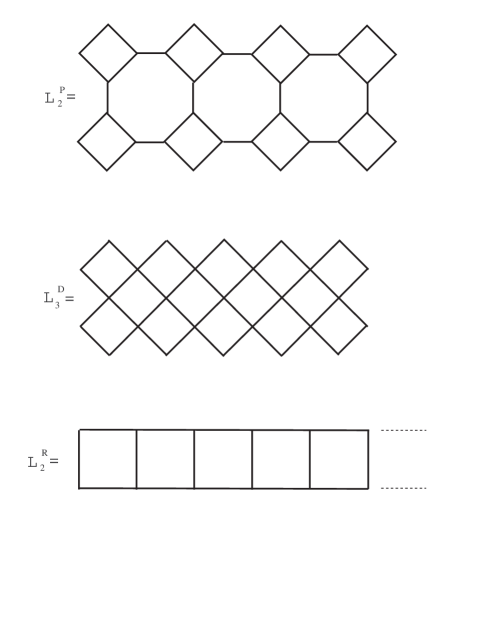
FIG. 22.: Several examples of related ladders as explained in text. (Above) An example of $(4,8)$-lattice with $n_{p}=2$ plaquettes. (Middle) An example of diagonal ladder with $n_{p}=3$ plaquettes. (Down) An example of rectangular ladder with $n_{=}2$ legs.

As shown in the previous section the limit $t_{d}\rightarrow\infty$ has the geometric significance of shrinking the corresponding $t_{d}$-links into sites, so that the the lattice ${\cal L}^{P}_{n_{p}}$ “renormalizes” into the diagonal ladder ${\cal L}_{2n_{p}-1}^{D}$ (see Fig. 22). In this strong coupling limit the number of plaquettes actually increases and some plaquettes are generated for free. The number of plaquettes of the diagonal ladder so obtained is odd. This construction does not produce even plaquette diagonal ladders.

Observe that all the diagonal ladders are bipartite lattices but only when $n_{p}$ is even are the number of sites of the two different sublattices the same. This suggests that the $n_{p}$-even diagonal AFH ladders belong to the same universality class as the $n_{l}$-even rectangular ladders, while the $n_{p}$-odd diagonal ladders belong to a different universality class characterized by ferrimagnetic GS’s.

The opposite limit, where $t_{d}\rightarrow 0$, has the geometrical meaning of shrinking the plaquettes into sites, so that ${\cal L}^{P}_{n_{p}}$ “renormalizes” the system to a rectangular ladder with $n_{p}$ legs ( see Fig. 22).

We summarize the above geometric RG operations in the following symbolic manner,

$$\begin{array}[]{lcll}{\cal L}^{P}_{n_{p}}&\longrightarrow&{\cal L}_{2n_{p}-1}^{D}&(t_{d}\rightarrow\infty)\\ {\cal L}^{P}_{n_{p}}&\longrightarrow&{\cal L}_{n_{p}}^{R}&(t_{d}\rightarrow 0)\end{array}$$ (36)

In this sense the $(4,8)$ lattice is an interpolating structure between diagonal and rectangular lattices.

There is an interesting connection between this plaquette construction and the theory of medial graphs. Consider a graph $G$ made of a set of points $i$ connected by links $<i,j>$. A medial graph ${\cal M}(G)$, associated with the graph $G$, is obtained by surrounding every site $i$ of $G$ by a polygon $P_{i}$, such that two polygons $P_{i}$ and $P_{j}$, which correspond to a link $<i,j>$, meet at a single intersection point $P_{i}\cap P_{j}$, which lies on the middle of the link $<i,j>$[23] (see Fig. 23 for a generic example).

Choosing the polygons $P_{i}$ to be 4-gons, i.e. plaquettes, one can easily show that a diagonal ladder with an odd number of plaquettes is the medial graph of a rectangular ladder, namely

$${\cal L}^{D}_{2n_{p}-1}=\;{\cal M}({\cal L}^{R}_{n_{p}})$$ (37)

Medial graphs are used in Statistical Mechanics to show the equivalence between the Potts model and the 6-vertex model[24, 23]. Indeed one can show that the Potts model defined on a graph $G$ is equivalent, i.e. has the same partition function after appropriate identification of parameters, to the 6 vertex model defined on the medial graph ${\cal M}(G)$, i.e.

$$Z_{\rm Potts}(G)=Z_{6-{\rm vertex}}({\cal M}(G))$$ (38)

The transformation $G\rightarrow{\cal M}(G)$ is a kind of duality map that relates two seemingly unrelated models and it is in fact the key to solve the 2D critical Potts model in terms of the 6 vertex one.

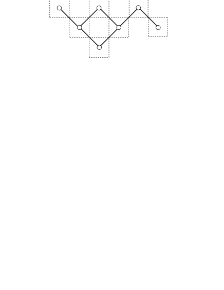
FIG. 23.: An example of medial graph construction. Here the graph G is made by solid lines and blank circles. Its associated medial graph ${\cal M}(G)$ is made by dashed lines.

B Plaquette Construction of the 2D Square Lattice

In Fig. 24 we apply the plaquette construction to the 2D square lattice. It is a simple generalization of the construction shown in the previous subsection when $n_{p}\rightarrow\infty$. If ${\cal L}^{D}_{\infty}$ is a square lattice with lattice spacing $a$, then ${\cal L}^{R}_{\infty}$ is also a square lattice but with spacing $\sqrt{2}a$ [25].

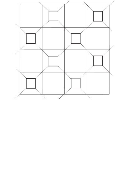
FIG. 24.: Plaquette constrution (small interior squares plus dashed lines) of the 2D square lattice as explained in text.

Let $x$ be the doping of a $t-J$ model defined on ${\cal L}^{D}_{\infty}$, and ${x}_{p}$ the doping factor of a $t_{p}-J_{p}-t_{d}$ model defined on ${\cal L}^{P}_{\infty}$, then the relations between these quantities are analogous to Eqs.(26) and (28) for the necklace ladder, namely

$$x=(2{x}_{p}-1)$$ (39)

$$t=\frac{1}{2}\;t_{p},\;\;\;J=\frac{1}{4}\;J_{p}$$ (40)

Eq.(39) implies that the undoped system $x=0$ corresponds to doping $x_{p}=1/2$ in the enlarged lattice. Fig. 25 shows a plaquette construction of the Néel state from the $x_{p}=1/2$ state. Notice that the plaquettes have spin 1 and that the parity on their diagonals alternate between $(1,-1)$ and $(-1,1)$. In the strong hopping limit the plaquettes have an effective spin 1. The whole set of these effective spin 1’s are coupled antiferromagnetically and form a square lattice with lattice spacing which is $\sqrt{2}$ times larger than the lattice spacing of the original spin 1/2 model. In a certain sense the plaquette construction integrates out degrees of freedom and renormalizes the system into an AF Heisenberg model with spin 1 and lattice space $\sqrt{2}a$. This picture agrees qualitatively with the RG flow of the $O(3)$ non linear sigma model in the renormalized classical region at zero temperature[26].

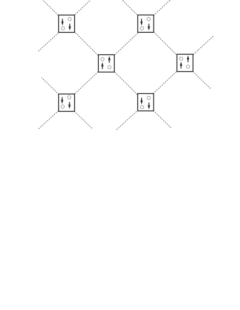
FIG. 25.: Plaquette constrution of the 2D Neel state in a square lattice as explained in text. The corresponding depicted state on the decorated (dual) lattice has doping $x_{p}=1/2$ and spin 1 on every small square plaquette.

In the weak hopping limit, however the GS of the 2D model is given essentially by the coherent superposition of localized Cooper pairs used in the construction of the $x=1/3$ necklace state. The Gutzwiller projection of this state onto the original lattice will produce Spin Peierls state rather than an AFLRO state.

We conclude that unlike the case of the necklace ladder, the $t_{p}-J_{p}-t_{d}$ model in 2D must have a phase transition for some intermediate value of $t_{d}$. The study of this model may serve to clarify the relationship between the AFLRO and the d-wave pairing structures observed in the theoretical models of strongly correlated systems.

IX Conclusions

Diagonal $t-J$ ladders provide an alternative route of interpolating between 1 and 2 spatial dimensions. Here we have described a general framework for such an interpolation and introduced a generalized $t_{p}-J_{p}-t_{d}$ plaquette model in which the individual plaquettes are linked by a hopping term $t_{d}$. In the strong hopping $t_{d}\gg t_{p},J_{p}$ limit, the generalized plaquette model was shown to map into the original diagonal $t-J$ model with renormalized parameters and filling factor. Thus, the generalized $t_{p}-J_{p}-t_{d}$ model provides a dual model to the original diagonal model. In this sense, it is interesting to study the $t_{p}-J_{p}-t_{d}$ model in the weak hopping limit. If there is no phase transition between the weak and strong hopping limits, then the weak hopping limit can provide new insight into the nature of the original $t-J$ diagonal ladder. We believe that this is the case for the $n_{p}=1$ plaquette necklace ladder and that its groundstate for a doping $x=\frac{1}{3}$ can be understood as the Gutzwiller projection of a product state of Cooper pairs localized on the plaquettes of the quarter-filled extended $t_{p}-J_{p}-t_{d}$ model. Alternatively, for the $n_{p}\to\infty$ 2D limit, we believe that the extended $t_{p}-J_{p}-t_{d}$ model at a doping $x_{p}=\frac{1}{2}$, which corresponds to the undoped $(x=0)$ $t-J$ model, will have a phase transition for an intermediate value of $t_{d}/t_{p}$. In this case, our conjecture is that the strong coupling limit will have a ground state with long range AF order while the weak coupling phase will be a localized Spin Peierls state.

In order to make these ideas more concrete, we have focused on the single plaquette $n_{p}=1$ necklace ladder. Here, using the results of DMRG and RVA calculations, we have studied the necklace ladder for various dopings $x$. For $x=\frac{1}{3}$, the DMRG calculations show that in the most probable configuration, the holes occupy the sites along the principal diagonal of the necklace and the spins form perfect singlets along the minor diagonals. The RVA calculations, starting from a “classical” configuration and mixing in local quantum fluctuations about this state, provide a ground state energy in good agreement with the DMRG result. Then, as discussed above, a more transparent physical picture of the $x=\frac{1}{3}$ state of the diagonal necklace is provided by the extended $t_{p}-J_{p}-t_{d}$ dual model at a filling of $x_{p}=\frac{1}{2}$ in which this state is seen as a localized Cooper pair state. It will be interesting to understand what happens when additional holes are added. In particular, will a necklace with a doping of $x_{p}=0.5+\delta$ have power law $d$-wave like pairing correlations?

For $x=0$, the diagonal necklace is equivalent to an alternating $s=1/s=\frac{1}{2}$ spin chain and has a ferrimagnetic ground state with total spin $N/2$, with $N$ the number of unit cells of the necklace. There are gapped excitations with spin $N/2+1$ and gapless excitations with spin $N/2-1$. In the weak hopping limit of the $t_{p}-J_{p}-t_{d}$ model, these excitations correspond to local excitations of the plaquettes to a spin $3/2$ state and to magnons of a ferromagnetic spin $\frac{1}{2}$ chain respectively. Thus, in the $x=0$ case, the dual model provides a useful physical picture.

We also have found that when the $x=\frac{1}{3}$ state is doped with holes, the ground state plaquettes retain the even parity characteristic of the $x=\frac{1}{3}$ state. However, when electrons are added, this parity can be even or odd. Thus, it appears that the $x=\frac{1}{3}$ doping separates the system into two distinct regions.

Clearly, the diagonal ladders form a rich class of models with properties ranging from ferrimagnetic to antiferromagnetic and from localized pair states to possible extended pairing states. Furthermore, the $t_{p}-J_{p}-t_{d}$ model provides a dual description which suggests alternative physical pictures and approximation schemes as well as connections to concepts from statistical mechanics.

Acknowledgements We would like to acknowledge useful discussions with Hsiu-Hau Lin and Eric Jeckelmann. GS would like to thank the members of the Physics Department of the UCSB for their warm hospitality. GS and MAMD acknowledges support from the DGES under contract PB96-0906, SRW acknowledges support from the NSF under Grant No.DMR-9509945, DJS acknowledges support from the NSF under Grant No. DMR-9527304 and JD acknowledges support from the DIGICYT under contract PB95/0123.

Appendix A: RVA approach to the necklace ladder

The RVA method is a kind of simplified DMRG where one retains a single state as the best candidate for the GS of the system. As in the DMRG the GS of a given length is constructed recursively from the states defined in previous steps. This idea can be implemented analytically if the ansatz is sufficiently simple. Below we shall propose various RVA states for the necklace ladder with dopings $0\leq x\leq 1/3$.

FIG. 26.: A pictorical view of the necklace ladder showing the labelling convention employed to denote the variational RVA states. Here the positions along the main (horizontal) diagonal of the ladder are sing odd sites, while the even positions are made up of rungs or sudiagonals.

A Case $x=0$

Let us begin by labelling the sites of the necklace ladder as in Fig. 26. The even sites denote the minor diagonal of the ladder while the odd sites are those on the principal diagonal.

At zero doping there are only two possible states on the odd sites given by,

$$|\uparrow>=c^{\dagger}_{\uparrow}\;|0>,\;\;\;\ |\downarrow>=c^{\dagger}_{\downarrow}\;|0>$$ (41)

On the even sites there are a triplet and a singlet state given by,

$$\begin{array}[]{cl}|S>=&\Delta_{1,2}^{\dagger}\;|0>\\ |T_{\uparrow}>=&c^{\dagger}_{1,\uparrow}\;c^{\dagger}_{2,\uparrow}\;|0>\\ |T_{\downarrow}>=&c^{\dagger}_{1,\downarrow}\;c^{\dagger}_{2,\downarrow}\;|0>\\ |T_{0}>=&\frac{1}{\sqrt{2}}(c^{\dagger}_{1,\uparrow}\;c^{\dagger}_{2,\downarrow}-c^{\dagger}_{1,\downarrow}\;c^{\dagger}_{2,\uparrow})\;|0>\end{array}$$ (42)

The Néel state on the necklace ladder can be written simply as,

$$|\downarrow>\;|T_{\uparrow}>\;|\downarrow>\;|T_{\uparrow}>\;\cdots|\downarrow>\;|T_{\uparrow}>\;|\downarrow>\;|T_{\uparrow}>\$$ (43)

A trivial observation is that the Néel state on the necklace with $N$ sites is generated by the first order recurrence relation,

$$|{\rm Neel},2N+1>=|\downarrow>\;\;|{\rm Neel},2N>$$ (44)

$$|{\rm Neel},2N>=|T_{\uparrow}>\;|{\rm Neel},2N-1>$$ (45)

Quantum fluctuations around the Néel state amount to local changes of the form (see Fig. 27)

$$|\downarrow>\;|T_{\uparrow}>\longrightarrow|(\downarrow,T_{\uparrow})>\equiv|\uparrow>\;|T_{0}>$$ (46)

$$|T_{\uparrow}>\;|\downarrow>\longrightarrow|(T_{\uparrow},\downarrow)>\equiv|T_{0}>\;|\uparrow>$$ (47)

$$|\downarrow>\;|T_{\uparrow}>\;|\downarrow>\longrightarrow|(\downarrow,T_{\uparrow},\downarrow)>\equiv|\uparrow>\;|T_{\downarrow}>\;|\uparrow>$$ (48)

Hence a globally perturbed Néel state is a coherent superposition of states of the form,

$$\downarrow\;(T_{\uparrow}\downarrow)(T_{\uparrow}\;\downarrow)\;T_{\uparrow}\;(\downarrow\;T_{\uparrow}\downarrow)\;(T_{\uparrow}\downarrow)T_{\uparrow}\;\downarrow\;(T_{\uparrow}\;\downarrow)\;T_{\uparrow}\downarrow$$ (49)

where the parenthesis denote the quantum fluctuations given in (47). The RVA state is a linear superposition of states of the type (49) weighted with probability amplitudes which are the variational parameters.

The RVA state is generated by the following recursion relations (RR),

$$\begin{array}[]{rl}|2N+1>=&|\downarrow>\;\;|2N>\\ &+u\;|(\downarrow,\;T_{\uparrow})>\;|2N-1>\\ &+v\;|(\downarrow,T_{\uparrow},\downarrow)>|2N-2>\\ |2N>=&|T_{\uparrow}>\;|2N-1>\\ &+u\;|(T_{\uparrow},\downarrow)>\;;|2N-2>\end{array}$$ (50)

with the initial condition

$$|N=1>\equiv|\downarrow>,\;\;\;|N=0>\equiv 1$$ (51)

To compute the energy of the state $|N>$ we define the following matrix elements,

$$Z_{N}=<N|N>$$ (52)

$$E_{N}=<N|H_{N}|N>$$ (53)

where $H_{N}$ is the Hamiltonian of the system with $N$ sites.

The RR’s for the states (50) imply a set of recursion relations for the matrix elements (52). Form the norm we get,

$$Z_{2N+1}=Z_{2N}+u^{2}Z_{2N-1}+v^{2}Z_{2N-2}$$ (54)

$$Z_{2N}=Z_{2N-1}+u^{2}Z_{2N-2}$$ (55)

The initial conditions are,

$$Z_{0}=Z_{1}=1$$ (56)

The RR’s for the energy are,

$$\begin{array}[]{rl}E_{2N+1}=&E_{2N}+u^{2}E_{2N-1}+v^{2}E_{2N-2}+\\ &J(\sqrt{2}u-{1\over 2})Z_{2N-1}+J(2\sqrt{2}uv-v^{2})Z_{2N-2}\\ &+{J\over 2}v^{2}Z_{2N-3}\\ E_{2N}=&E_{2N-1}+u^{2}E_{2N-2}+\\ &J(\sqrt{2}u-{1\over 2})Z_{2N-2}+Ju^{2}Z_{2N-3}{J\over 2}v^{2}Z_{2N-4}\end{array}$$ (62)

while in this case the initial data are

$$E_{0}=E_{1}=0$$ (63)

Minimizing the GS energy in the limit $N>>1$ we find that the GS per plaquette is given by -0.4822 J, which corresponds to an energy per site of the associated spin chain equal to -0.7233 J. The values of the variational parameters are given by $u=-0.3288$ and $v=0.1691$.

B Case $x=1/3$

The most probable state for this doping is given by (see Fig. 7)

$$|\circ>\;|S>\;|\circ>\;|S>\;\cdots|\circ>\;|S>\;|\circ>$$ (64)

Analogously to Eq.(47) we define local fluctuations around (64) in terms of the states $|(\circ,S)>,|(S,\circ)>$ and $|(\circ,S,\circ)>$ depicted in Fig. 27. The $x=1/3$ RVA state can then be constructed from the following RR’s ( see Fig. 17)

$$\begin{array}[]{rl}|2N+1>=&|\circ>\;\;|2N>\\ &+a\;|(\circ,\;S)>\;|2N-1>\\ &+b\;|(\circ,S,\circ)>|2N-2>\\ |2N>=&|S>\;|2N-1>\\ &+a\;|(S,\circ)>\;|2N-2>\end{array}$$ (65)

The norm of $|N>$ satisfies the RR’s (54) with the replacements $u\rightarrow a,v\rightarrow b$. The RR’s for the energy matrix elements are given by,

$$E_{2N+1}=E_{2N}+a^{2}E_{2N-1}+b^{2}E_{2N-2}$$ (66)

$$+(\sqrt{2}(-2t)a-Ja^{2})Z_{2N-1}+\sqrt{2}(-2t)2abZ_{2N-2}$$ (67)

$$+a^{2}(-J/4)(a^{2}Z_{2N-3}+b^{2}Z_{2N-4})$$ (68)

$$+b^{2}(-J/4)(2Z_{2N-3}+a^{2}Z_{2N-4})$$ (69)

$$E_{2N}=E_{2N-1}+a^{2}E_{2N-2}-(2\sqrt{2}ta+Ja^{2})Z_{2N-2}$$ (70)

$$(-J/4)(a^{2}Z_{2N-3}+2b^{2}Z_{2N-4})$$ (71)

$$+a^{2}(-J/4)(2Z_{2N-3}+a^{2}Z_{2N-4})$$ (72)

The initial conditions for both $Z_{N}$ and $E_{N}$ are the same as for the undoped case. In the limit $N\rightarrow\infty$ we find

$$\lim_{N\rightarrow\infty}\frac{E_{0}(N)}{N}=-0.7387,\;\;\;a=0.7873,\;\;\;b=0.5478$$ (73)

which give the asymptotic values of the curves in Fig. 18.

FIG. 27.: A pictorical representation of fluctuation states as constructed in text for the RVA method in the necklace ladder. Here $T_{+}$ and $T_{-}$ stand for $T_{\uparrow}$ and $T_{\downarrow}$, respectively.

C Cases $0<x<1/3$

In the underdoped region $0<x<1/3$ we have observed with the DMRG that many of the GS that one gets, and particularly those listed in Table 2 can be understood as quantum fluctuations around a “classical” state $|\psi_{0}>$. This state has the generic structure already seen in the cases $x=0$ and 1/3 (see (49) and (64)), namely

$$|\psi_{0}\rangle=|l_{2N+1}\rangle|l_{2N}\rangle\cdots|l_{2}\rangle|l_{1}\rangle$$ (74)

where the states $|l_{i}\rangle$, $i=1,2,\cdots 2N,2N+1$, are taken to be

$$|l_{odd}\rangle=\{|0\rangle,|\downarrow\rangle,|\uparrow\rangle\}=\{1,3,5\}$$ (75)

$$|l_{even}\rangle=\{|S\rangle,|T_{\uparrow}\rangle,|T_{\downarrow}\rangle\}=\{2,4,6\}$$ (76)

Notice that we do not allow the holes on the minor diagonals of the classical state $|\psi_{0}>$. They will go there after considering the fluctuations [22]. Based on the DMRG results as well as physical considerations, we shall allow the following pairs $|l_{i}>|l_{i+1}>$ in $|\psi_{0}>$

$$|0\rangle|S\rangle,\;|0\rangle|T_{\uparrow}\rangle,\;|\downarrow\rangle|T_{\uparrow}\rangle,\;|0\rangle|T_{\downarrow}\rangle,\;|\uparrow\rangle|T_{\downarrow}\rangle$$ (77)

$$|S\rangle|0\rangle,\;|T_{\uparrow}\rangle|0\rangle,\;|T_{\uparrow}\rangle|\downarrow\rangle,\;|T_{\downarrow}\rangle|0\rangle,\;|T_{\downarrow}\rangle|\uparrow\rangle$$ (78)

FIG. 28.: A pictorical representation of fluctuation states as constructed in text for the RVA method in the necklace ladder. Here $T_{+}$ and $T_{-}$ stand for $T_{\uparrow}$ and $T_{\downarrow}$, respectively.

FIG. 29.: A pictorical representation of fluctuation states as constructed in text for the RVA method in the necklace ladder. Here $T_{+}$ and $T_{-}$ stand for $T_{\uparrow}$ and $T_{\downarrow}$, respectively.

This connectivity of the states making up a certain $|\psi_{0}\rangle$ state can be summarized in a graph in which we place a site for each and every 6 states in (75), (76), and joint them by links whenever it is possible to find them one next to each other in the $|\psi_{0}\rangle$ state according to the allowed local configurations (77,78). This graph is depicted in Fig. 30, and coincides with the Dynkin diagram of the exceptional Lie Group $E_{6}$.

Now we can characterize every admissible classical state $|\psi_{0}\rangle$ in a geometrical fashion: each $|\psi_{0}\rangle$ is a path in the so called Bratelli diagram associated to the Dynkin diagram of $E_{6}$. This Bratelli diagram is shown in Fig. 31. The way it is constructed is apparent in that figure: one starts with the 3 possible site-states (75) located one on top of each other. These states are located by the label $l_{1}$ of the first site of the diagonal ladder. Then we link them to the 3 possible rung-states (76) according to the connectivity prescribed in Fig. 30. These rung-states are located by the label $l_{2}$ of the second position of the diagonal ladder. Once this is achieved, the rest of the graph in Fig. 31 is made up by reflecting this basic piece over the rest of the labels $l_{3},l_{4},\ldots,l_{2N},l_{2N+1}$. Observe that the $x=0$ and $x=1/3$ states discussed previously correspond to straight paths of the Bratelli diagram (34). A similar type of construction is also used in Statistical Mechanics in the context of the Face Models[23].

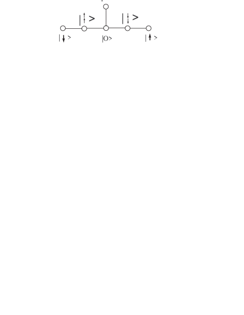
FIG. 30.: Dynkin diagram of the exceptional Lie group $E_{6}$ and its associated site and rung states contributing to the variational RVA method for the necklace ladder. These 6 states make up every classical state $|\psi_{0}\rangle$ on the underdoped ladder according to the connectivity of this diagram.

The quantum fluctuations around $|\psi_{0}>$ amounts to considering the normalized states $|(l_{i},l_{i+1})>$ and $|(l_{i},l_{i+1},l_{i+2})>$ depicted in Figs. 27-29. An interesting property of these states is that they are orthogonal, i.e.

$$\langle l_{j}|(l_{i},l_{i+1},l_{i+2})\rangle=0,\;\;j=i,i+1,i+2$$ (79)

$$\langle(l_{j},l_{j+1})|(l_{i},l_{i+1},l_{i+2})\rangle=0,\;\;j=i,i+1$$ (80)

The RVA state built upon $|\psi_{0}>$ is generated by the RR’s, (see Fig. 30)

$$\begin{array}[]{rl}|2N+1\rangle=&|l_{2N+1}\rangle|2N\rangle+a_{N}|(l_{2N+1},l_{2N})\rangle|2N-1\rangle\\ &+b_{N}|(l_{2N+1},l_{2N},l_{2N-1})\rangle|2N-2\rangle\\ &\\ |2N\rangle=&|l_{2N}\rangle|2N-1\rangle+c_{N}|(l_{2N},l_{2N-1})\rangle|2N-2\rangle\end{array}$$ (85)

provided with the initial data,

$$|1\rangle\equiv|l_{1}\rangle,\;|0\rangle\equiv 1$$ (86)

Using the orthogonality conditions (79,80) it is easy to get the RR’s satisfied by the norm of the RVA state

$$Z_{2N+1}=Z_{2N}+a_{N}^{2}Z_{2N-1}+b_{N}^{2}Z_{2N-2}$$ (87)

$$Z_{2N}=Z_{2N-1}+c_{N}^{2}Z_{2N-2}$$ (88)

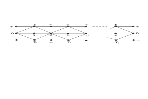
FIG. 31.: Bratelli diagram of the exceptional Lie group $E_{6}$. It serves to classify all the classical states $\psi_{0}$ appearing in the RVA treatment of the underdoped necklace ladder: every path on this diagram characterizes one of those classical states and provides its quantum numbers. Here $T_{+}$ and $T_{-}$ stand for $T_{\uparrow}$ and $T_{\downarrow}$, respectively. Also, $S$ denotes a singlet state and $O$ represents a hole.

The RR’s for the energy have the structure given below

$\displaystyle E_{2N+1}=E_{2N}+a_{N}^{2}E_{2N-1}+b_{N}^{2}E_{2N-2}+$

$\displaystyle Z_{2N-1}(\epsilon_{2N+1,2N}^{(0)}+a_{N}^{2}\epsilon_{2N+1,2N}^{(2)}$

$\displaystyle+2a_{N}\epsilon_{2N+1,2N}^{(1)})+$

$\displaystyle Z_{2N-2}(c_{N}^{2}\epsilon_{2N+1,2N,2N-1}^{(4)}+$

$\displaystyle a_{N}^{2}\bar{\epsilon}_{2N+1,2N,2N-1}^{(4)}+b_{N}^{2}\epsilon_{2N+1,2N,2N-1}^{(8)}+$

$\displaystyle 2b_{N}c_{N}\epsilon_{2N+1,2N,2N-1}^{(3)}+2a_{N}b_{N}\bar{\epsilon}_{2N+1,2N,2N-1}^{(3)})+$

$\displaystyle Z_{2N-3}(a_{N}^{2}a_{N-1}^{2}\epsilon_{2N+1,2N,2N-1,2N-2}^{(5)}+$

$\displaystyle b_{N}^{2}\bar{\epsilon}_{2N+1,2N,2N-1,2N-2}^{(6)})+$

$\displaystyle Z_{2N-4}(a_{N}^{2}b_{N-1}^{2}\epsilon_{2N+1,2N,2N-1,2N-2,2N-3}^{(7)}+$

$$b_{N}^{2}c_{N-1}^{2}\bar{\epsilon}_{2N+1,2N,2N-1,2N-2,2N-3}^{(7)})$$ (89)

$\displaystyle E_{2N}=E_{2N-1}+c_{N}^{2}E_{2N-2}$

$\displaystyle+Z_{2N-2}(\epsilon_{2N,2N-1}^{(0)}+c_{N}^{2}\epsilon_{2N,2N-1}^{(2)}+2c_{N}\epsilon_{2N,2N-1}^{(1)})+$

$\displaystyle Z_{2N-3}(a_{N-1}^{2}\epsilon_{2N,2N-1,2N-2}^{(4)}$

$\displaystyle+c_{N}^{2}\bar{\epsilon}_{2N,2N-1,2N-2}^{(4)})+$

$\displaystyle Z_{2N-4}(b_{N-1}^{2}\epsilon_{2N,2N-1,2N-2,2N-3}^{(6)}$

$$+c_{N}^{2}c_{N-1}^{2}\epsilon_{2N,2N-1,2N-2,2N-3}^{(5)})$$ (90)

The $\epsilon$ symbols in Eqs. (90) are reduced energy matrix elements involving the states defined in Fig. 27-29. To simplify the RR’s for the energy we adopt the notation: $\epsilon_{2N+1,2N,\dots}\equiv\epsilon_{l_{2N+1},l_{2N},\dots}$, where $l_{2N+1},l_{2N},\dots$ run over the six possible states, $1,\dots,6$, of the Dynkin diagram $E_{6}$. All the non vanishing values of $\epsilon$ are shown in tables 3.

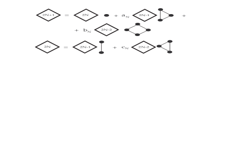
FIG. 32.: A pictorical representation of the Recursion Relations in Eq. (85) employed to generate the variational states in the RVA treatment of the underdoped ($0\leq x\leq 1/3$) necklace ladder. Here $a$, $b$ and $c$ are local variational parameters. A square denotes a bulk state on a ladder of a length given by its number inside. The black circles and solid lines represent generic fluctuation states as explained in the text.

Given the previous equations we set up the following strategy to derive the results presented in Section V.

• Fix the length $N$ of the ladder, the number of holes $h$ and the third component of the spin $S^{z}$ of the whole ladder.

• Generate all the $|\psi_{0}>$

  configurations with those quantum numbers $N,h,S^{z}$. Generically the number of configurations grows exponentially. For example the 7 plaquette case studied in Section V has N=15 and a total of $3\times 10^{4}$ configurations.

• Compute the energy of the state associated with the zero-order state $|\psi_{0}>$ using the recursion relations and find the variational parameters which lead to a minimum energy. For example for the 7 plaquette ladder we used 21 independent variational parameters.

• Extract the state $|\psi_{0}>$ which has the absolute minimum energy for a given $N,h$ and $S^{z}$.

$\epsilon_{i_{1},i_{2}}^{(0)}$	(3,4), (5,6),(4,3),(6,5)	$-J$
$\epsilon_{i_{1},i_{2}}^{(1)}$	(1,2),(1,4),(1,6),(2,1),(4,1),(6,1)	$-\sqrt{2}t$
$\epsilon_{i_{1},i_{2}}^{(1)}$	(3,4),(5,6),(4,3),(6,5)	${J\over\sqrt{2}}$
$\epsilon_{i_{1},i_{2}}^{(2)}$	(1,2),(2,1)	$-J$
$\epsilon_{i_{1},i_{2}}^{(2)}$	(3,4),(5,6),(4,3),(6,5)	$-{J\over 2}$

Table 3 a) Non-vanishing reduced energy matrix elements for $\epsilon_{i_{1},i_{2}}^{(0)}=\langle l_{i_{2}}|\langle l_{i_{1}}|h^{(tJ)}_{i_{1}i_{2}}|l_{i_{1}}\rangle|l_{i_{2}}\rangle$ where the tJ Hamiltonian acts only on the states specified by its subscripts. Likewise for the elements $\epsilon_{i_{1},i_{2}}^{(1)}=\langle(l_{i_{1}}l_{i_{2}})|h^{(tJ)}_{i_{1}i_{2}}|l_{i_{1}}\rangle|l_{i_{2}}\rangle$, $\epsilon_{i_{1},i_{2}}^{(2)}=\langle(l_{i_{1}}l_{i_{2}})|h^{(tJ)}_{i_{1}i_{2}}|(l_{i_{1}},l_{i_{2}})\rangle$.

$\epsilon_{i_{1},i_{2},i_{3}}^{(3)}$	(1,2,1)	$-\sqrt{2}t$
$\epsilon_{i_{1},i_{2},i_{3}}^{(3)}$	(1,4,3),(1,6,5)	$-t$
$\epsilon_{i_{1},i_{2},i_{3}}^{(3)}$	(3,4,1),(5,6,1)	${-J\over 2}$
$\epsilon_{i_{1},i_{2},i_{3}}^{(3)}$	(3,4,3),(5,6,5)	${J\over\sqrt{2}}$
$\bar{\epsilon}_{i_{1},i_{2},i_{3}}^{(3)}$	(1,2,1)	$-\sqrt{2}t$
$\bar{\epsilon}_{i_{1},i_{2},i_{3}}^{(3)}$	(1,4,3),(1,6,5)	${J\over 2}$
$\bar{\epsilon}_{i_{1},i_{2},i_{3}}^{(3)}$	(3,4,1),(5,6,1)	$t$
$\bar{\epsilon}_{i_{1},i_{2},i_{3}}^{(3)}$	(3,4,3),(5,6,5)	${J\over\sqrt{2}}$

Table 3 b) Non-vanishing reduced energy matrix elements for $\epsilon_{i_{1},i_{2},i_{3}}^{(3)}=\langle(l_{i_{1}},l_{i_{2}},l_{i_{3}})|h^{(tJ)}_{i_{1}i_{2}}|l_{i_{1}}\rangle|(l_{i_{2}},l_{i_{3}})\rangle$ where the tJ Hamiltonian acts only on the states specified by its subscripts. Likewise for the elements $\bar{\epsilon}_{i_{1},i_{2},i_{3}}^{(3)}=\langle(l_{i_{1}},l_{i_{2}},l_{i_{3}})|h^{(tJ)}_{i_{2}i_{3}}|(l_{i_{1}},l_{i_{2}})\rangle|l_{i_{3}}\rangle$.

$\epsilon_{i_{1},i_{2},i_{3}}^{(4)}$	(2,1,2),(2,1,4),(2,1,6),(4,1,2),(6,1,2)	$-{J\over 2}$
$\epsilon_{i_{1},i_{2},i_{3}}^{(4)}$	(3,4,3),(5,6,5),(3,4,1),(5,6,1)	-${J\over 2}$
$\epsilon_{i_{1},i_{2},i_{3}}^{(4)}$	(6,1,4),(4,1,6)	$J$
$\bar{\epsilon}_{i_{1},i_{2},i_{3}}^{(4)}$	(2,1,2),(2,1,4),(2,1,6),(4,1,2),(6,1,2)	$-{J\over 2}$
$\bar{\epsilon}_{i_{1},i_{2},i_{3}}^{(4)}$	(3,4,3),(5,6,5),(1,4,3),(1,6,5)	$-{J\over 2}$
$\bar{\epsilon}_{i_{1},i_{2},i_{3}}^{(4)}$	(4,1,6),(6,1,4)	$J$

Table 3 c) Non-vanishing reduced energy matrix elements for $\epsilon_{i_{1},i_{2},i_{3}}^{(4)}=\langle(l_{i_{2}},l_{i_{3}})|\langle l_{i_{1}}|h^{(tJ)}_{i_{1}i_{2}}|l_{i_{1}}\rangle|(l_{i_{2}},l_{i_{3}})\rangle$ where the tJ Hamiltonian acts only on the states specified by its subscripts. Likewise for the elements $\bar{\epsilon}_{i_{1},i_{2},i_{3}}^{(4)}=\langle l_{i_{3}}|\langle(l_{i_{1}},l_{i_{2}})|h^{(tJ)}_{i_{2}i_{3}}|(l_{i_{1}},l_{i_{2}})\rangle|l_{i_{3}}\rangle$.

$\epsilon_{i_{1},i_{2},i_{3}}^{(8)}$	(3,4,3),(5,6,5)	$-2J$
$\epsilon_{i_{1},i_{2},i_{3}}^{(8)}$	(1,4,3),(1,6,5),(3,4,1),(5,6,1)	$-J$

Table 3 d) Non-vanishing energy matrix elements $\epsilon_{i_{1},i_{2},i_{3}}^{(8)}=\langle(l_{i_{1}},l_{i_{2}},l_{i_{3}})|(h^{(tJ)}_{i_{1}i_{2}}+h^{(tJ)}_{i_{2}i_{3}})|(l_{i_{1}},l_{i_{2}},l_{i_{3}})\rangle$ where the tJ Hamiltonian acts only on the states specified by its subscripts. .

$\epsilon_{i_{1},i_{2},i_{3},i_{4}}^{(5)}$	(1,2,1,2),(1,2,1,4),(1,2,1,6),(1,4,1,2),(1,6,1,2)	$-{J\over 4}$
$\epsilon_{i_{1},i_{2},i_{3},i_{4}}^{(5)}$	(1,4,1,6),(1,6,1,4),(3,4,3,4),(5,6,5,6),(3,4,1,2)	$-{J\over 2}$
$\epsilon_{i_{1},i_{2},i_{3},i_{4}}^{(5)}$	(5,6,1,2),(3,4,1,6),(5,6,1,4),(3,4,1,4),(5,6,1,6)	$-{J\over 2}$
$\epsilon_{i_{1},i_{2},i_{3},i_{4}}^{(5)}$	(2,1,2,1),(2,1,4,1),(2,1,6,1),(4,1,2,1),(6,1,2,1)	$-{J\over 4}$
$\epsilon_{i_{1},i_{2},i_{3},i_{4}}^{(5)}$	(2,1,4,3),(2,1,6,5),(4,3,4,3),(6,5,6,5),(4,1,4,3)	$-{J\over 2}$
$\epsilon_{i_{1},i_{2},i_{3},i_{4}}^{(5)}$	(6,1,6,5),(4,1,6,1),(6,1,4,1),(4,1,6,5),(6,1,4,3)	$-{J\over 2}$

Table 3 e) Non-vanishing energy matrix elements $\epsilon_{i_{1},i_{2},i_{3},i_{4}}^{(5)}=\langle(l_{i_{3}},l_{i_{4}})|\langle(l_{i_{1}},l_{i_{2}})|h^{(tJ)}_{i_{2}i_{3}}|(l_{i_{1}},l_{i_{2}})\rangle|(l_{i_{3}},l_{i_{4}})\rangle$ where the tJ Hamiltonian acts only on the states specified by its subscripts.

$\epsilon_{i_{1},i_{2},i_{3},i_{4}}^{(6)}$	(2,1,2,1),(2,1,4,1),(2,1,6,1),(2,1,4,3),(2,1,6,5)	$-{J\over 2}$
$\epsilon_{i_{1},i_{2},i_{3},i_{4}}^{(6)}$	(4,1,2,1),(6,1,2,1),(4,1,6,5),(6,1,4,3)	$-{J\over 2}$
$\epsilon_{i_{1},i_{2},i_{3},i_{4}}^{(6)}$	(4,1,6,1),(6,1,4,1)	$-J$

Table 3 f) Non-vanishing energy matrix elements $\epsilon_{i_{1},i_{2},i_{3},i_{4}}^{(6)}=\langle(l_{i_{2}},l_{i_{3}},l_{i_{4}})|\langle l_{i_{1}}|h^{(tJ)}_{i_{1}i_{2}}|l_{i_{1}}\rangle|(l_{i_{2}},l_{i_{3}},l_{i_{4}})\rangle$ where the tJ Hamiltonian acts only on the states specified by its subscripts.

$\bar{\epsilon}_{i_{1},i_{2},i_{3},i_{4}}^{(6)}$	(1,2,1,2),(1,2,1,4),(1,2,1,6),(1,4,1,2),(1,6,1,2)	$-{J\over 2}$
$\bar{\epsilon}_{i_{1},i_{2},i_{3},i_{4}}^{(6)}$	(3,4,1,2),(5,6,1,2),(3,4,1,6),(5,6,1,4)	$-{J\over 2}$
$\bar{\epsilon}_{i_{1},i_{2},i_{3},i_{4}}^{(6)}$	(1,4,1,6),(1,6,1,4)	$-J$

Table 3 g) Non-vanishing energy matrix elements $\bar{\epsilon}_{i_{1},i_{2},i_{3},i_{4}}^{(6)}=\langle l_{i_{4}}|\langle(l_{i_{1}},l_{i_{2}},l_{i_{3}})|h^{(tJ)}_{i_{3}i_{4}}|(l_{i_{1}},l_{i_{2}},l_{i_{3}})\rangle|l_{i_{4}}\rangle$ where the tJ Hamiltonian acts only on the states specified by its subscripts.

$\epsilon_{i_{1},i_{2},i_{3},i_{4},i_{5}}^{(7)}$	(1,2,1,2,1),(1,2,1,4,1),(1,2,1,6,1),(1,2,1,4,3)	$-{J\over 4}$
$\epsilon_{i_{1},i_{2},i_{3},i_{4},i_{5}}^{(7)}$	(1,2,1,6,5),(1,4,1,2,1),(1,6,1,2,1)	$-{J\over 4}$
$\epsilon_{i_{1},i_{2},i_{3},i_{4},i_{5}}^{(7)}$	(1,4,1,6,1),(1,6,1,4,1),(1,4,1,6,5),(1,6,1,4,3)	$-{J\over 2}$
$\epsilon_{i_{1},i_{2},i_{3},i_{4},i_{5}}^{(7)}$	(3,4,3,4,3),(5,6,5,6,5),(3,4,3,4,1),(5,6,5,6,1)	$-{J\over 2}$
$\epsilon_{i_{1},i_{2},i_{3},i_{4},i_{5}}^{(7)}$	(3,4,1,2,1),(5,6,1,2,1),(3,4,1,4,3),(5,6,1,6,5)	$-{J\over 2}$
$\epsilon_{i_{1},i_{2},i_{3},i_{4},i_{5}}^{(7)}$	(3,4,1,4,1),(5,6,1,6,1),(3,4,1,6,5)	$-{J\over 2}$
$\epsilon_{i_{1},i_{2},i_{3},i_{4},i_{5}}^{(7)}$	(5,6,1,4,3),(3,4,1,6,1),(5,6,1,4,1)	$-{J\over 2}$

Table 3 h) Non-vanishing reduced energy matrix elements for $\epsilon_{i_{1},i_{2},i_{3},i_{4},i_{5}}^{(7)}=\langle(l_{i_{3}},l_{i_{4}},l_{i_{5}})|\langle(l_{i_{1}},l_{i_{2}})|h^{(tJ)}_{i_{2}i_{3}}|(l_{i_{1}},l_{i_{2}})\rangle|(l_{i_{3}},l_{i_{4}},l_{i_{5}})\rangle$ where the tJ Hamiltonian acts only on the states specified by its subscripts.

$\bar{\epsilon}_{i_{1},i_{2},i_{3},i_{4},i_{5}}^{(7)}$	(1,2,1,2,1),(1,4,1,2,1),(1,6,1,2,1),(3,4,1,2,1)	$-{J\over 4}$
$\bar{\epsilon}_{i_{1},i_{2},i_{3},i_{4},i_{5}}^{(7)}$	(5,6,1,2,1),(1,2,1,4,1),(1,2,1,6,1)	$-{J\over 4}$
$\bar{\epsilon}_{i_{1},i_{2},i_{3},i_{4},i_{5}}^{(7)}$	(1,6,1,4,1),(1,4,1,6,1),(5,6,1,4,1),(3,4,1,6,1)	$-{J\over 2}$
$\bar{\epsilon}_{i_{1},i_{2},i_{3},i_{4},i_{5}}^{(7)}$	(3,4,3,4,3),(5,6,5,6,5),(1,4,3,4,3),(1,6,5,6,5)	$-{J\over 2}$
$\bar{\epsilon}_{i_{1},i_{2},i_{3},i_{4},i_{5}}^{(7)}$	(1,2,1,4,3),(1,2,1,6,5),(3,4,1,4,3),(5,6,1,6,5)	$-{J\over 2}$
$\bar{\epsilon}_{i_{1},i_{2},i_{3},i_{4},i_{5}}^{(7)}$	(1,4,1,4,3),(1,6,1,6,5),(5,6,1,4,3)	$-{J\over 2}$
$\bar{\epsilon}_{i_{1},i_{2},i_{3},i_{4},i_{5}}^{(7)}$	(3,4,1,6,5),(1,6,1,4,3),(1,4,1,6,5)	$-{J\over 2}$

Table 3 i) Non-vanishing reduced energy matrix elements for $\bar{\epsilon}_{i_{1},i_{2},i_{3},i_{4},i_{5}}^{(7)}=\langle(l_{i_{4}},l_{i_{5}})|\langle(l_{i_{1}},l_{i_{2}},l_{i_{3}})|h^{(tJ)}_{i_{3}i_{4}}|(l_{i_{1}},l_{i_{2}},l_{i_{3}})\rangle|(l_{i_{4}},l_{i_{5}})\rangle$ where the tJ Hamiltonian acts only on the states specified by its subscripts.

D Electronic Density G.S. Expectation Values

Here we derive the general equations to compute the electronic density expectation values using the RVA method. In particular, we have plotted in Fig. 8 the results for the doping case $x=1/3$ in the necklace ladder and compared it with the DMRG results showing a good agreement.

Let us denote the density electronic operator at the site position $R$ as $d_{R}$, namely,

$$d_{R}=n_{R,\uparrow}+n_{R,\downarrow}$$ (91)

where $n_{R,\uparrow}$ and $n_{R,\downarrow}$ are the number operators for fermions with spins up and down, respectively.

For a diagonal ladder of length $N$ (sites+rungs) we need to compute the V.E.V. of the density operator $d_{R}$ in the ground state, which we denote as,

$$d_{N}(R)=\langle N|d_{R}|N\rangle$$ (92)

When the position $R$ is even we shall need an additional index $k=1,2$ to locate the upper site ($k=1$) and the lower site ($k=2$) of the rung.

Notice that these density V.E.V. (92) are not normalized. We may introduce normalized densities as,

$$\hat{d}_{N}(R)={\langle N|d_{R}|N\rangle\over\langle N|N\rangle}={d_{N}(R)\over Z_{N}}$$ (93)

The densities $\hat{d}_{N}(R)$ takes on values from 0 to 1 depending on whether we find a hole with maximum probability ($\hat{d}_{N}(R)=0$) or one electron ($\hat{d}_{N}(R)=1$).

Using the RR’s for the diagonal (85) ladder we may find also RR’s for the unnormalized V.E.V.’s:

$$d_{2N+1}(R)=d_{2N}(R)+a_{N}^{2}d_{2N-1}(R)+b_{N}^{2}d_{2N-2}(R)$$ (94)

$$d_{2N}(R)=d_{2N-1}(R)+c_{N}^{2}d_{2N-2}(R)$$ (95)

whenerver the position $R$ of the insertion is not near the end of the diagonal ladder state. The derivation of these RR’s follow closely that of the norms $Z^{\prime}s$ using the orthogonality relations.

Now we need to determine the boundary or initial conditions to feed those RR’s. Let us consider the cases $R$ odd and even separately.

1 $R$ Odd

As for the odd sites the RR’s of the states are third order, we have to compute directly the values $d_{R}(R)$, $d_{R+1}(R)$ and $d_{R+2}(R)$. Clearly we also have,

$$d_{R-1}(R)=0$$ (96)

Now, as $R$ is odd, let us set $R=2r+1$. Then, using the RR’s we find,

$$d_{2r+1}(2r+1)=\delta_{2r+1}^{(o)}Z_{2r}+a_{r}^{2}Z_{2r-1}+b_{r}^{2}Z_{2r-2}$$ (97)

In the derivation of these RR’s we need to compute the following reduced density matrix elements,

$$\delta_{2r+1}^{(o)}\equiv\langle l_{2r+1}|d_{2r+1}|l_{2r+1}\rangle=\left\{\begin{array}[]{ccc}0&\mbox{if}&l_{2r+1}=|\circ\rangle\\ 1&\mbox{if}&l_{2r+1}=\{|\uparrow\rangle,|\downarrow\rangle\}\end{array}\right.$$ (98)

$$\delta_{2r+1,2r}^{(o)}\equiv\langle(l_{2r+1},l_{2r})|d_{2r+1}|(l_{2r+1},l_{2r})\rangle=1$$ (99)

$\displaystyle\delta_{2r+1,2r,2r-1}^{(o)}\equiv$

$$\langle(l_{2r+1},l_{2r},l_{2r-1})|d_{2r+1}|(l_{2r+1},l_{2r},l_{2r-1})\rangle=1$$ (100)

Likewise we proceed with the initial value $d_{R+1}(R)$ and we find,

$$d_{2r+2}(2r+1)=d_{2r+1}(2r+1)+c_{r+1}^{2}Z_{2r}$$ (101)

where we have used the result,

$$\langle(l_{2r+2},l_{2r+1})|d_{2r+1}|(l_{2r+2},l_{2r+1})\rangle=1$$ (102)

Finally, we proceed similarly with the other initial value $d_{R+2}(R)$ and we find,

$\displaystyle d_{2r+3}(2r+1)=d_{2r+2}(2r+1)+$

$$a_{r+1}^{2}d_{2r+1}(2r+1)+b_{r+1}^{2}Z_{2r}$$ (103)

2 $R$ Even

As for the even positions (rungs) the RR’s (85) of the states are second order, we have to compute directly the values $d_{R}(R,k)$ and $d_{R+1}(R,k)$ ($k=1,2$). Clearly we also have,

$$d_{R-1}(R,k)=0$$ (104)

Now, as $R$ is even, let us set $R=2r$. Then, using the RR’s we find,

$$d_{2r}(2r,k)=Z_{2r-1}+c_{r}^{2}\delta_{2r,2r-1,k}^{(e)}Z_{2r-2}$$ (105)

In the derivation of these RR’s we need to compute the following reduced density matrix elements,

$$\delta_{2r,k}^{(e)}\equiv\langle l_{2r}|d_{2r,k}|l_{2r}\rangle=1$$ (106)

$$\delta_{2r,2r-1,k}^{(e)}\equiv\langle(l_{2r},l_{2r-1})|d_{2r,k}|(l_{2r},l_{2r-1})\rangle$$ (107)

Using the expressions of the fluctuation states $|(l_{2r},l_{2r-1})\rangle$ we find that the only nonvanishing elements are as follows,

$$\begin{array}[]{ccc}\delta_{1,2;k}^{(e)}={1\over 2},&\delta_{1,4;k}^{(e)}={1\over 2},&\delta_{1,6;k}^{(e)}={1\over 2}\end{array}$$ (108)

$$\begin{array}[]{ccc}\delta_{2,1;k}^{(e)}={1\over 2},&\delta_{4,1;k}^{(e)}={1\over 2},&\delta_{6,1;k}^{(e)}={1\over 2}\end{array}$$ (109)

$$\begin{array}[]{cc}\delta_{3,4;k}^{(e)}=1,&\delta_{5,6;k}^{(e)}=1\end{array}$$ (110)

$$\begin{array}[]{cc}\delta_{4,3;k}^{(e)}=1,&\delta_{6,5;k}^{(e)}=1\end{array}$$ (111)

where we are following the notation for the site/rung states, $\{1,3,5\}=\{|\circ\rangle,|\downarrow\rangle,|\uparrow\rangle\}$, $\{2,4,6\}=\{|S\rangle,|T_{\uparrow}\rangle,|T_{\downarrow}\rangle\}$.

Likewise we proceed with the other initial value $d_{R+1}(R)$ and we find,

$\displaystyle d_{2r+1}(2r,k)=d_{2r}(2r,k)+$

$$a_{r}^{2}\delta_{2r+1,2r,k}^{(e)}Z_{2r-1}+b_{r}^{2}\delta_{2r+1,2r,2r-1,k}^{(e)}Z_{2r-2}$$ (112)

In the derivation of these RR’s we need to compute the following reduced density matrix elements,

$$\delta_{2r+1,2r,2r-1,k}^{(e)}\equiv\langle(l_{2r+1},l_{2r},l_{2r-1})|d_{2r,k}|(l_{2r+1},l_{2r},l_{2r-1})\rangle$$ (113)

Using the expressions of the fluctuation states $|(l_{2r+1},l_{2r},l_{2r-1})\rangle$ we find that the only nonvanishing elements are as follows,

$$\begin{array}[]{cc}\delta_{3,4,3;k}^{(e)}=1,&\delta_{5,6,5;k}^{(e)}=1\end{array}$$ (114)

$$\begin{array}[]{cc}\delta_{3,4,1;k}^{(e)}={1\over 2},&\delta_{5,6,1;k}^{(e)}={1\over 2}\end{array}$$ (115)

$$\begin{array}[]{cc}\delta_{1,4,3;k}^{(e)}={1\over 2},&\delta_{1,5,6;k}^{(e)}={1\over 2}\end{array}$$ (116)

Appendix B: Spectrum of the $t-j$ model on the plaquette

The $t-J$ Hamiltonian on the plaquette has the symmetry group $D_{4}$ of the square. This implies that the eigenstates can be classified with the irreps of $D_{4}$, together with the number of holes $h$ and the total spin $S$. $D_{4}$ has 5 irreps, four of which are one-dimensional $A_{1},B_{1},A_{2},B_{2}$ and one two-dimensional irrep $E$. From the character table of this group one sees that the irreps $A_{1},B_{1}$ have, in our terminology, even parity in both diagonals, while the irreps $A_{2},B_{2}$ are odd. The parity of the states in the irrep $E$ is $(+,-)$ and $(-,+)$ for the two diagonals. In Table 3 we show the analytic expression of the energy and the value for the cases $J=0$ and $J=0.5$ ($t=1)$. In Fig. 33 we show a plot with all the energies as functions of $J/t$. Observe the crossover between the lowest energy states at $J/t\sim 1.37$.

$h$	$S$	$D_{4}$	Energy	$J=0$	$J=0.5$
0	0	$B_{2}$	$-3J$	0	$-1.5$
0	1	$A_{2}$	$-2J$	0	$-1$
0	0	$A_{1}$	$-J$	0	$-0.5$
0	1	$E$	$-J$	0	$-0.5$
0	2	$B_{2}$	0	0	0
1	1/2	$E$	$-J-\sqrt{3t^{2}+J^{2}/4}$	$-\sqrt{3}$	$-2.25$
1	1/2	$B_{2}$	$-3J/2-t$	$-1$	$-1.75$
1	1/2	$B_{1}$	$-J/2-t$	$-1$	$-1.25$
1	1/2	$A_{2}$	$-3J/2+t$	1	0.25
1	1/2	$A_{1}$	$-J/2+t$	1	0.75
1	1/2	$E$	$-J+\sqrt{3t^{2}+J^{2}/4}$	$\sqrt{3}$	1.25
1	3/2	$A_{2}$	$-2t$	$-2$	$-2$
1	3/2	$E$	0	0	0
1	3/2	$B_{2}$	$2t$	2	2
2	0	$A_{1}$	$-J/2-\sqrt{8t^{2}+J^{2}/4}$	$-\sqrt{8}$	$-3.09$
2	0	$B_{1}$	$0$	0	$0$
2	0	$E,B_{2}$	$-J$	0	$-0.5$
2	0	$A_{1}$	$-J/2+\sqrt{8t^{2}+J^{2}/4}$	$\sqrt{8}$	2.59
2	1	$E$	$-2t$	$-2$	$-2$
2	1	$A_{2},B_{1}$	$0$	0	0
2	1	$E$	$2t$	2	2
3	1/2	$A_{1}$	$-2t$	$-2$	$-2$
3	1/2	$E$	$0$	0	0
3	1/2	$B_{1}$	$2t$	2	2
4	0	$A_{1}$	0	0	0

Table 4. Here $h$ is the number of holes, $S$ the total spin, The third column denotes the irrep of the $D_{4}$ group. We give the values of the energy for $J=0$ and 0.5 ( $t=1$).

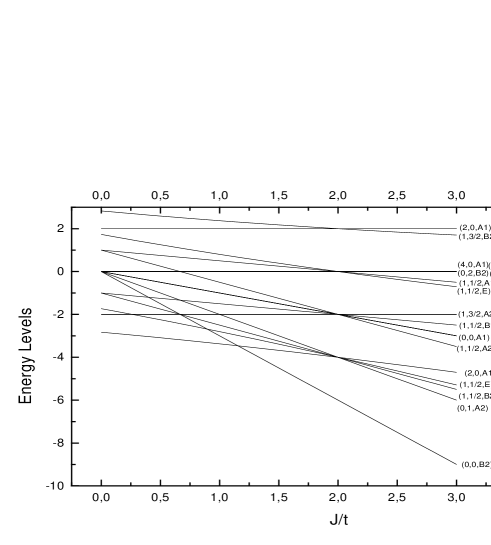
FIG. 33.: Plot showing the energy levels for a $tJ$ model on the $2\times 2$ plaquette as a function of the coupling $J/t$. The energy levels are classified according the $D_{4}$ symmetry group of the square as shown in table 4.

Appendix C: Plaquette derivation of the equivalence between the Haldane state and the RVB state of the 2-leg spin ladder

There has been some debate in the past as to whether the Haldane state of the spin 1 chain is in the same phase as the GS of the AFH 2-leg ladder. The general consensus is that they both belong to the same universality class characterized by a spin gap, finite spin correlation length and non vanishing string order parameter. The DMRG study of Ref. [27] demonstrated a continuous mapping between these systems, and pointed out the equivalence between a dimer-RVB state on a composite spin model (which is a ladder model with some extra hopping terms) and the AKLT model.

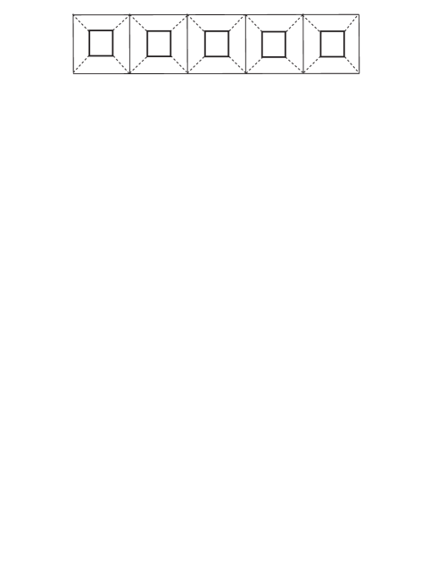
FIG. 34.: Plaquette construction (small interior squares plus dashed lines) of the rectangular ladder with $n_{l}=2$ legs.

This suggests that there must be a direct way to relate the valence bond construction of the spin 1 AKLT state[18] and the dimer-RVB picture of the 2-leg ladder[28, 16]. We shall show that this is indeed possible through the plaquette construction of the 2-leg ladder, which is shown diagrammatically in Figs. 34 and 35.

In Fig. 34 the 2-leg ladder is split into plaquettes connected by two links. We have generalized somewhat the medial construction in this case, since two plaquettes are allowed to have more than one common link. The interesting point is that the filling factor $x$ of the ladder and the one of the extended model, $x_{p}$, are related in exactly the same manner as the 2D lattices (see Eq.(39)). Thus $x=0$ corresponds to $x_{p}=1/2$. Let us assume for the moment that each plaquette has spin 1. Then the effective interaction describing the coupling of these spins will be an AFH model. This suggests that we can construct a valence bond state to approximate the plaquette ground state by drawing nearest neighbors bonds among the elementary spins between plaquettes, as shown in the upper part of Fig. 35. Now, if we project out of this state any $S=0$ components of each plaquette, we get the AKLT state, where each plaquette is a pure spin $S=1$. If, instead, we Gutzwiller project the $t_{d}$ links, as shown in Fig. 35, we get the dimer-RVB state proposed in references[28, 16].

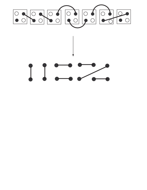
FIG. 35.: (Below) A dimer-RVB state on a rectangular 2-leg ladder obtained as the projection (above) of a doped $x_{p}=1/2$ valence bond state on the decorated (dual) lattice associated to the rectangular ladder.

Hence, the plaquette model acts as intermediate system, for which different projections generate either the AKLT state of the spin-1 chain or the dimer-RVB state of the two-leg ladder.

REFERENCES

- [1] E. Dagotto and T. M. Rice, Science 271, 619 (1996)
- [2] M. Greven, R.J. Birgeneau and U.-J.Wiese, Phys. Rev. Lett. 77, 1865 (1996); G. Sierra, J. Phys. A 29, 3299 (1996); S. Chakravarty, Phys. Rev. Lett. 77, 4446 (1996); O.F. Syljuasen, S. Chakravarty, and M. Greven, condmat/9701197.
- [3] M. Azuma, Z. Hiroi, M. Takano, K. Ishida, and Y. Kataoka, Phys. Rev. Lett. 73, 3463 (1994); S.A. Carter, B. Battlogg, R.J. Cava, J.J. Krajewski, W.F. Peck, Jr., and T.M. Rice, Phys. Rev. Lett. 77, 1378 (1996).
- [4] J. M. Tranquada et al. Nature 375, 561 (1995); Phys. Rev. B 54, 7489 (1996).
- [5] J. Zaanen and O. Gunnarsson, Phys. Rev. B40, 7391 (1989); D. Poilblanc and T.M. Rice, Phys. Rev. B39, 9749 (1989); H.J. Schulz, J. Physique, 50, 2833 (1989); K. Machida, Physica C 158, 192 (1989); K. Kato et. al., J. Phys. Soc. Jpn. 59, 1047 (1990); J.A. Vergés et. al., Phys. Rev. B43, 6099 (1991); M. Inui and P.B. Littlewood, Phys. Rev. B44, 4415 (1991); J. Zaanen and A.M. Oles, Ann. Physik 5, 224, (1996).
- [6] S.R. White, Phys. Rev. Lett.69, 2863 (1992), Phys. Rev. B48, 10345 (1993).
- [7] S. R. White and D.J Scalapino, Phys. Rev. Lett. 80, 1272 (1998); and cond-mat/9801274.
- [8] U. Brandt and A. Giesekus, Phys. Rev. Lett. 68, 2648 (1992).
- [9] H. Tasaki, Phys. Rev. Lett. 70, 3303 (1993).
- [10] A. Giesekus, Phys. Rev. B 52, 2476, (1995).
- [11] M. Uehara , T. Nagata, J. Akimitsu, H. Takahashi, N. Mori and K. Kinoshita, J. of Phys. Jpn, 65,2764 (1997).
- [12] S.K. Pati, S. Ramasesha and D. Sen, Phys. Rev. B55, 8894 (1997) and cond-mat/9704057.
- [13] A.K. Kolezhuk, H.-J. Mikeska and S. Yamamoto, Phys. Rev. B55, 3336 (1997).
-
[14]
S. Yamamoto, S. Brehmer and H.-J. Mikeska, cond-mat/9710332.
S. Brehmer, H.-J. Mikeska and S. Yamamoto, cond-mat/9610109. - [15] A. Klumper, A. Schadschneider and J. Zittartz, Europhys. Lett. 24, 293 (1993).
- [16] G. Sierra and M.A. Martin-Delgado, Phys. Rev. B 56, 8774 (1997).
- [17] G. Sierra, M.A. Martin-Delgado, J. Dukelsky, S. R. White and D. J. Scalapino, Phys. Rev.B 57, 11666 (1998).
- [18] I. Affleck, T. Kennedy, E. H. Lieb and H. Tasaki, Commun. Math. Phys. 115, 477 (1988).
- [19] S.R. White and D.J. Scalapino, Phys. Rev. B 55, 6504 (1997).
- [20] J. Gonzalez, M.A. Martin-Delgado, G. Sierra and A.H. Vozmediano, “Quantum Electron Liquids and High-Tc Superconductivity” Chapter 11, Lecture Notes in Physics, Monographs vol. 38, Springer-Verlag 1995.
- [21] The link Hamiltonian (18) can be written in terms of the bonding and antibonding operators as . Hence the 4 states and have zero energy and are in one-to-one correspondence with those of a Hubbard model while the remaining 12 states, which contain antibonding operators, decouple in the limit .
- [22] This election of states to construct the ground state in the RVA method depends on the coupling regime under consideration. Here we are assuming throughout this paper so that kinetics effects are stronger that exchange effects. Were we in a regime with , then the selection of building states would be different. The physics of the problem dictates the way in which the RVA method is set up.
- [23] R.J. Baxter, “Exactly Solved Models in Statistical Mechanics”, Academic Press, London (1982).
- [24] H. Temperley and E. Lieb, Proc. Roy. Soc. (London) 251 (1971).
- [25] The planes of the cuprates yield another example of medial construction. Let and denote the square lattices formed by the and ions respectively. Then the lattice is the medial graph of the lattice, i.e. . A plaquette corresponds in this case to a single ion surrounded by 4 Oxigens. This implies that the 3 band Hubbard model admits a natural -extension.
- [26] S. Chakravarty, B.I. Halperin and D.R. Nelson, Phys. Rev. Lett. 60, 1057 (1988), Phys. Rev. B 39, 2344 (1989).
- [27] S. R. White, Phys. Rev. B 53, 52 (1996).
- [28] S.R. White, R.M. Noack and D.J. Scalapino, Phys. Rev. Lett. 73, 886 (1994).