Superflow in $d$-wave superconductors

Abstract

Superflow in a phenomenological tight-binding model for the superconducting state of some High-temperature superconductors is discussed thoroughly. The formalism used is explicitly gauge-invariant and currents are computed exactly within BCS theory, going therefore beyond linear response theory. The dependence of gap functions, current density, critical currents and free energy as a function of the superfluid velocity for different angles and doping concentrations is investigated. Different sources of anisotropy, like the dispersion relation of the model, the internal symmetry of the order parameter, and orthorhombic distortions of the lattice are also studied.

Introduction

Kamerlingh Onnes discovered some ninety years ago that the resistivity of certain metals would drop to zero when the temperature was lowered below a critical value $T_{c}$. He accordingly termed superconductors all materials which exhibited such state of disipationless electric flow. Superconductors display as a matter of fact a rich variety of physical phenomena other than superflow, some of which are closely related to it, like the Meissner effect, some others having a different nature, as the electronic gap which appears in tunneling experiments.

Superflow and Meissner’s effects are a consequence of the London equation, a linear relation between the density current and the vector potential, $\vec{\j}+{\sf K}\,\vec{A}=0$, which serves to define the current response tensor ${\sf K}$. Such an equation, or its non-local version, holds in a superconductor even in the presence of the usual scattering mechanisms which degrade the current in a normal metal. A conventional exercise consists in solving London and Maxwell’s equations in a specific geometry to find the distribution of current densities and magnetic fields. [1, 2] It is shown in this way that they are highly nonuniform across the sample: they are confined to a thin shell in contact to the surface and do not penetrate the bulk of the sample.

Interestingly enough, superflow and Meissner’s effects might be the most difficult properties to extract from the microscopic BCS theory of superconductivity, because the derivation of the London equation is not an easy task. The standard procedure to derive this relation uses linear response theory. [3] One complication arises from the fact that such expression is not gauge invariant, so that a change in the longitudinal part of $\vec{A}$ will change $\vec{\j}_{l}$. The longitudinal response kernel ${\sf K}_{l}$ is in turn related to the density response function through the continuity equation, so the problem of gauge invariance can also be stated as a problem of charge conservation. Within linear response theory, BCS theory must therefore be extended to enforce the Ward Identity which relates the dressed vertex of the longitudinal response function ${\sf K}_{l}$ to the BCS self-energy.[3] It can also be proven that any explicit computation of superflow in a superconductor must be fully self-consistent in order to ensure that charge is conserved.[4, 5]

The superflow state can be destroyed by increasing the current density, the magnetic field, or the temperature above certain critical values which depend among other things on the specific material used, the amount of disorder of the sample, or the geometry of the device which is used. Furthermore, the relation between $\vec{\j}$ and $\vec{A}$ is not linear for large $\vec{\j}$. In other words, London’s equation does not hold close to the critical value of the superflow current density, ${\rm j}_{c}$. The situation in strong type II superconductors is even more complicated because the magnetic field originated by the supercurrent might give rise to vortices; these vortices move in the presence of the supercurrent and dissipate energy.[6]

Superflow in High-temperature superconductors might be anisotropic because (a) the order parameter has $d$-wave symmetry; (b) the electronic structure is also fairly anisotropic, with van Hove singularities slightly below the Fermi energy;[7, 8] (c) the two-dimensional ${\sf Cu\,O_{2}}$ planes, responsible for much of the physics of the cuprates, present different types of orthorhombic distortions. The purpose of this article is to study the physics of superflow in clean, infinite, $d$-wave superconductors on an orthorhombically distorted square lattice. A phenomenological two-dimensional tight-binding model which captures some of the experimental features of the superconducting state of High-temperature superconductors will be used.[9, 10] No attention will be paid to the effects of disorder, twin boundaries, or external or induced magnetic fields, all of which can be important in this compounds and will be dealt with in the near future. Superflow in two-dimensional $d$-wave superconductors has already been studied using a Ginsburg-Landau approach, which focused in particular on the induction of non-$d$-wave components upon switching on of the current.[11] Superflow in quasi-one-dimensional $s$-wave superconductors has also been studied in equilibrium[12, 13] and non-equilibrium situations.[14, 15]

Section II is devoted to present the model and the formalism used to solve it in the presence of a finite superflow. The mapping onto a linearized isotropic model is also shown. Section III discusses the results obtained for the phase diagram of the model, the gaps, their distortion due to orthorhombic effects and the local density of states, for zero current density. Section IV is devoted to study the doping and angular dependence of the gaps, free energy, current density, and critical current in the presence of a superflow. A summary closes the article. Even though the analytical calculations have been performed using the Matsubara formalism, all the numerical results provided in the article correspond to T=0.

Formalism

The partition function of a superconducting sample in the presence of an electromagnetic field can be written as

$${\cal Z}(T,\mu)=\int{\cal D}[\Delta^{*},\Delta,\vec{A},A_{0}]\,e^{-\frac{1}{\hbar}\,{\cal S}[\Delta^{*},\Delta,\vec{A},A_{0}]}$$ (1)

where the functional integral sums over all possible configurations of order parameter and electromagnetic fields, $\Delta(x,x^{\prime})=|\Delta(x,x^{\prime})|\,e^{i\,(\phi(x)+\phi(x^{\prime}))},\,\vec{A(x)},\,A_{0}(x)$, and where the imaginary-time action is

$${\cal S} = \int dx\,dx^{\prime}\Bigl{[}-{\rm Tr}\,\ln\,\tilde{G}_{\sf e}^{-1}(x,x^{\prime})+\frac{|\Delta(x,x^{\prime})|^{2}}{V(x,x^{\prime})}$$ (4)

$$+\Bigl{(}e\,n_{i}\,A_{0}(x)+\frac{\vec{B}^{2}(x)-\vec{E}^{2}(x)}{8\,\pi}\Bigr{)}\,\delta(x-x^{\prime})\Bigr{]}+{\cal H}^{*}(0).$$

Here $x$ denotes the four vector $(\tau,\vec{x})$, $V(x,x^{\prime})=V(\vec{x}-\vec{x^{\prime}})\,\delta(\tau-\tau^{\prime})$ is the pairing potential, $e\,n_{i}$ is the background charge density of ions, $\tilde{G}_{\sf e}(x,x^{\prime})$ is the Green function of electrons in Nambu’s space,

$$\left(\begin{array}[]{cc}\Bigl{(}\hbar\,\partial_{\tau}+{\cal H}(x)\Bigr{)}\,\delta(x-x^{\prime})&\Delta(x,x^{\prime})\,\delta(\tau-\tau^{\prime})\\ \Delta^{*}(x,x^{\prime})\,\delta(\tau-\tau^{\prime})&\Bigl{(}\hbar\,\partial_{\tau}-{\cal H}^{*}(x)\Bigr{)}\,\delta(x-x^{\prime})\end{array}\right)^{-1},$$ (7)

and in the Hamiltonian

$${\cal H}(x)=\frac{(\vec{p}+e/c\,\vec{A}(x))^{2}}{2\,m}+v_{latt}(\vec{x})-e\,A_{0}(x)-\mu$$

the Zeeman term has been discarded.

It can be seen that the action is invariant under the following gauge U(1) symmetry

$$A_{0}(x) \mapsto A_{0}(x)-\frac{i\,\hbar}{2\,e}\partial_{\tau}\theta(x),$$ (8)

$$\vec{A}(x) \mapsto \vec{A}(x)+\frac{\hbar\,c}{2\,e}\vec{\nabla}\theta(x),$$ (9)

$$\phi(x) \mapsto \phi(x)-\frac{\theta(x)}{2},$$ (10)

up to a total time derivative.

The phase of the order parameter field can therefore be absorbed by the electromagnetic field, and drops out of the problem if one defines the gauge invariant quantities[16]

$$\Psi_{s}(x)=A_{0}(x)-\frac{i\,\hbar}{2\,e}\,\partial_{\tau}\,\phi(x),$$ (11)

$$\vec{v}_{s}(x)=\frac{\hbar}{2\,m}\left(\vec{\nabla}\phi(x)+\frac{2\,e}{\hbar\,c}\,\vec{A}(x)\right),$$ (12)

in terms of which the electric and magnetic fields are written as

$$\vec{E}(x)=-\vec{\nabla}\,\Psi_{s}(x)-\frac{i\,m}{e}\,\partial_{\tau}\,\vec{v}_{s}(x),$$ (13)

$$\vec{B}(x)=\frac{m\,c}{e}\,\vec{\nabla}\times\vec{v}_{s}(x).$$ (14)

As shown by van Otterlo and coworkers,[16] the whole problem can be rephrased using these new variables:

$${\cal Z}(T,\mu)=\int{\cal D}[\Delta_{l},\vec{v}_{s},\Psi_{s}]\,e^{-\frac{1}{\hbar}\,{\cal S^{\prime}}[\Delta_{l},\vec{v}_{s},\Psi_{s}]},$$ (15)

(16)

$${\cal S^{\prime}}=\int dx\,dx^{\prime}\Bigl{[}-{\rm Tr}\,\ln\,\tilde{G}_{\sf e}^{-1}(x,x^{\prime})+\frac{\Delta_{l}^{2}(x,x^{\prime})}{V(x,x^{\prime})}$$ (17)

$$+\Bigl{(}e\,n_{i}\,\Psi_{s}(x)+\frac{\vec{B}^{2}(x)-\vec{E}^{2}(x)}{8\,\pi}\Bigr{)}\,\delta(x-x^{\prime})\Bigr{]}+{\cal H}^{*}(0),$$ (18)

(19)

$$\tilde{G}_{\sf e}^{-1}=\left(\begin{array}[]{cc}\Bigl{(}\hbar\,\partial_{\tau}+{\cal H}\Bigr{)}\,\delta(x-x^{\prime})&\Delta_{l}\,\delta(\tau-\tau^{\prime})\\ \Delta_{l}\,\delta(\tau-\tau^{\prime})&\Bigl{(}\hbar\,\partial_{\tau}-{\cal H}^{*}\Bigr{)}\,\delta(x-x^{\prime})\end{array}\right),$$ (22)

(23)

$${\cal H}(\vec{x})=\frac{(\vec{p}+m\,\vec{v}_{s}(x))^{2}}{2\,m}+v_{latt}(\vec{x})-e\,\Psi_{s}(x)-\mu,$$ (24)

where $\Delta_{l}=|\Delta|$ is a real scalar field whose vacuum value will be different from zero below $T_{C}$ and the phase $\phi$ is explicitly linked to the dynamics of the electromagnetic fields and the Higgs mechanism through the longitudinal part of the superfluid velocity field, $\vec{v}_{s,l}$.

Stationarity of the action with respect to $\Delta_{l},\vec{v}_{s}$ and $\Psi_{s}$ leads to the saddle point equations which determine the classical configurations of electromagnetic and order parameter fields, and to the saddle point approximation for the thermodynamic potential

$$\vec{\nabla}\cdot\,\vec{E}_{cl}(x)=4\,\pi\,e(n_{i}-n_{e}(x)),$$ (26)

$$-\frac{i}{c}\partial_{\tau}\vec{E}_{cl}(x)+\vec{\nabla}\times\vec{B}_{cl}(x)=\frac{4\,\pi}{c}{\sf\vec{\j}}(x),$$ (27)

$$\Delta_{l,cl}(\vec{x},\vec{x^{\prime}})=-\frac{1}{L^{d}}\,V(\vec{x},\vec{x^{\prime}})\,G_{{\sf e},12}(\vec{x},\vec{x^{\prime}}),$$ (28)

$$\Omega_{SP}(T,\mu,\Delta_{l,cl},\vec{E}_{cl},\vec{B}_{cl})=\frac{1}{\beta\,\hbar}{\cal S}_{SP}^{\prime}[\Delta_{l,cl},\vec{E}_{cl},\vec{B}_{cl}],$$ (29)

where $L^{d}$ is the volume of the sample, and $G_{{\sf e},12}$ is the off-diagonal element of $\tilde{G}_{\sf e}$. The electronic and current densities are defined in terms of the diagonal elements of $G_{\sf e}$ as

$$n_{e}(x)=\frac{G_{{\sf e},11}(x,x)-G_{{\sf e},22}(x,x)}{L^{d}},$$ (31)

$${\vec{\j}}_{e}(x)=-\frac{e}{m\,L^{d}}\,Tr\,\left[\left(\vec{p}\,\tilde{\openone}+m\vec{v}_{s}(x)\,\tilde{\tau}_{z}\right)\,\tilde{G}_{\sf e}(x,y)\right]_{y=x},$$ (32)

where $\tilde{\tau}_{z}$ is the third Pauli matrix.

The saddle point equation for the order parameter can be further simplified by changing to center of mass and relative coordinates and performing the Fourier transform with respect to the relative coordinate. Then

$$\Delta_{l,cl}(\vec{k},\vec{R})=-\frac{1}{L^{d}}\sum_{\vec{k^{\prime}}}\,V(\vec{k}-\vec{k^{\prime}})\,G_{e,12}(\vec{k^{\prime}},\vec{R}).$$ (33)

Expanding now $\Delta_{l,cl}$ and $V$ in terms of some basis set of functions $\eta_{a}$ as can be, for instance, those which form the irreducible representations of a crystallographic point group,

$$\Delta_{l,cl}(\vec{k},\vec{R})=\sum_{a}\Delta_{a}(\vec{R})\,\eta_{a}(\vec{k}),$$ (34)

$$V(\vec{k}-\vec{k^{\prime}},\vec{R})=\sum_{a}V_{a}(\vec{R})\,\eta_{a}(\vec{k})\,\eta(\vec{k^{\prime}})$$ (35)

one easily finds that

$$\Delta_{a}(\vec{R})=-\frac{V_{a}(\vec{R})}{L^{d}}\sum_{\vec{k}}\,\eta_{a}(\vec{k})\,G_{e,12}(\vec{k},\vec{R}).$$ (36)

Superflow is a superconducting state characterized by the stationary flow of a current $\vec{\j}$ in the absence of any longitudinal electric field (neglecting that built up at the boundary of the specimen.) This implies in view of Eqs. (11) and (14) that $\Psi_{s}(x)$ is identically zero, and that the superfluid velocity $v_{s}(x)$ does not depend on time. This state is therefore determined by two classical fields, $\Delta_{l,cl}(\vec{x})$ and $\vec{v}_{s,cl}(\vec{x})$, which must be determined self-consistently with the aid of Eqs. (27) and (28).

In an infinite sample, with no externally applied fields, $\Delta_{l,cl}$ and $\vec{v}_{s,cl}$ are uniform, so that Eq. (27) drops out of the problem and the superfluid velocity is just an input parameter, which can be viewed as a Doppler shift acquired by the kinetic energy part of the Hamiltonian

$${\cal T}=\frac{(\vec{p}+m\,\vec{v}_{s})^{2}}{2\,m}=\frac{(\vec{p}+\hbar\,\vec{q})^{2}}{2\,m},$$ (37)

The order parameter field must still be determined and, once self-consistency is achieved, the current density can be computed via Eq. (32). The continuity equation, $\vec{\nabla}\cdot\vec{\j}=0$ is automatically satisfied in this case.

In a finite geometry with no constrictions, like a wire or a thin film, the full self-consistent problem must be handled, but there are some facts which simplify the computation: (a) $\vec{\j}(\vec{x})$ must always point in the same direction, say the Z axis, because of the symmetry of the problem. (b) The continuity equation then demands that $\vec{\j}$ and $\vec{v}_{s}$ vary only in the XY plane. Now, the continuity equation is automatically satisfied if the order parameter is calculated self-consistently.[4, 5] Therefore, any explicit self-consistent calculation conserves charge and is gauge invariant by construction if $\vec{\j}$ is computed using Eq. (32) with no further approximations like linear response theory.

For an infinite superconductor, the current density can also be obtained in a more direct fashion by calculating the gradient of the thermodynamic potential,

$$\vec{\j}[q]=-\frac{e}{\hbar\,L^{d-1}}\,\vec{\nabla}_{\vec{q}}\,\Omega_{SP}(T,\mu,[q]).$$ (38)

It is worth pointing out that a finite Doppler shift in the dispersion relation of a normal metal leads to no observable effects, because it can always be made disappear by performing a simple change of variables in the k-sums, $\vec{k}+\vec{q}\mapsto\vec{k}$. Indeed, a finite current can only be induced in a metal by applying a finite electric field.

The formalism developed so far is going to be applied to study the physics of superflow in a clean, infinite $d$-wave superconductor where the electromagnetic fields are zero or at least negligible. The electronic fields will be described by a phenomenological one-band Hubbard-like model on an orthorhombically distorted square lattice. [9, 10]

The dispersion relation used comes from a fit to the spectral peaks found in ARPES experiments of optimally doped ${\sf Bi_{2}Sr_{2}CaCu_{2}O_{8-\delta}}$. [9] The interactions among electrons $V(\vec{x}-\vec{x^{\prime}})$ are assumed to be different from zero only when $\vec{x}$ and $\vec{x^{\prime}}$ are the same site ($V(\vec{0})=V_{0}$) or when they are nearest neighbors ($V(\vec{x}-\vec{x^{\prime}})=V(\vec{\delta})=V_{1}$). Explicitly,

$${\cal H}= \sum_{\vec{k},\sigma}\left[\frac{1}{z}\sum_{\vec{\delta}}\,t(|\vec{\delta}|)\,e^{i\,\vec{k}\cdot\vec{\delta}}\,-\mu\right]\hat{c}_{\vec{k},\sigma}^{+}\,\hat{c}_{\vec{k},\sigma}$$ (40)

$$-\,V_{0}\,\sum_{i}\>\hat{c}_{i,\uparrow}^{+}\,\hat{c}_{i,\downarrow}^{+}\,\hat{c}_{i,\downarrow}\,\hat{c}_{i,\uparrow}\,-\,V_{1}\,\sum_{i,\delta^{\prime}}\>\hat{c}_{i,\uparrow}^{+}\,\hat{c}_{i+\delta^{\prime},\downarrow}^{+}\,\hat{c}_{i+\delta^{\prime},\downarrow}\,\hat{c}_{i,\uparrow},$$

where $z$ is the coordination number, the sum in $\vec{\delta}$ extends up to five nearest neighbors, the hopping integrals $t(|\vec{\delta}|)$ have the values [-595,164,-52,56,51] meV, and the chemical potential can be varied freely to change the mean occupation number $n$ of the band. It is therefore assumed that the band is shifted rigidly upon doping, a fact which is not inconsistent with the available data from ARPES experiments. [17]

Monte Carlo and RPA studies of the repulsive Hubbard model have found that the effective potential among dressed quasiparticles assumes an RKKY or ”Mexican hat” form [18] so that it has a large repulsive on-site contribution and then decays exponentially in an oscillating way. Within this magnetic scenario for superconductivity in the cuprates, [19] the length scale over which the potential varies is set by the magnetic coherence length $\xi_{mag}$ and is therefore uncommensurated with the lattice spacing $a$. The interaction term used in this article bears some resemblance with such an effective potential if the on-site interaction $V_{0}$ if assumed to be large and negative. The resulting effective model can then be thought of as a low energy fixed point Hamiltonian which appears after integrating out the high frequency degrees of freedom of a more complicated model describing the physics of the cuprates. The effective model can therefore be safely solved using Mean Field techniques.

Generically, the four possible one-dimensional irreducible representations of the group of the square $C_{4v}$ transform under its symmetry operations as the identity, $x^{2}-y^{2}$, $x\,y$ and $x\,y\,(x^{2}-y^{2})$. [20] Their explicit form in a tight-binding formulation would be $s$ or extended $s$ ($s^{*}$), $d_{x^{2}-y^{2}}$, $d_{xy}$, and $d_{xy}\times d_{x^{2}-y^{2}}$, states.

A Mean Field decomposition of the on-site interaction naturally gives rise to a pure $s$ or to a spin-density-wave (SDW) state, depending on whether $V_{0}$ is attractive or repulsive. A nearest neighbor attraction produces an $s^{*}$ and a $d_{x^{2}-y^{2}}$ state; a second nearest neighbors interaction $V_{2}$ gives rise to a second $s^{*}$ state and to the $d_{xy}$ state, and so on. The Mean Field solution of this Hamiltonian therefore allows for a SDW state, and superconducting $s$-wave, extended $s$-wave, $d$-wave states, and mixed representations of them ($s+s^{*},d+i(s+s^{*}),s+s^{*}+d$). Similar results have been obtained in Refs. [21, 22, 23, 24].

The saddle point equations for the thermodynamic potential, the order parameter, the occupation of the band and the Helmholtz free energy per site are

$$\frac{\Omega_{SP}(T,\mu)}{M}= \frac{|\Delta_{s}|^{2}}{V_{0}}+\frac{|\Delta_{s^{*}}|^{2}+|\Delta_{d}|^{2}}{V_{1}}$$ (44)

$$+\frac{1}{M}\sum_{\vec{k}}\left[\xi_{\vec{k}+\vec{q}}-E_{\vec{k},\vec{q}}-\frac{2}{\beta}\ln(1+e^{-\beta E_{\vec{k},\vec{q}}})\right],$$

$$\Delta_{a}=\frac{V_{a}}{M}\sum_{\vec{k}}\frac{\Delta_{\vec{k}}\,\eta_{a,\vec{k}}}{2E_{\vec{k},\vec{q}}}\tanh\left(\frac{\beta E_{\vec{k},\vec{q}}}{2}\right),$$ (45)

$$n=\frac{N}{M}=\sum_{\vec{k}}\left[1-\frac{\xi_{\vec{k}+\vec{q}}+\xi_{\vec{k}-\vec{q}}}{2\,E_{\vec{k},\vec{q}}}\tanh\left(\frac{\beta E_{\vec{k},\vec{q}}}{2}\right)\right],$$ (46)

$$f_{SP}(T,n)=\frac{\Omega_{BCS}(T,\mu(n))}{M}+\mu(n)\,n,$$ (47)

where the dispersion relation for the quasiparticles is

$$E_{\vec{k},\vec{q}} = \frac{\xi_{\vec{k}+\vec{q}}-\xi_{\vec{k}-\vec{q}}}{2}+\sqrt{\left(\frac{\xi_{\vec{k}+\vec{q}}+\xi_{\vec{k}-\vec{q}}}{2}\right)^{2}+|\Delta_{\vec{k}}|^{2}},$$ (48)

$$\Delta_{\vec{k}} = \sum_{a=s,s^{*},d}\Delta_{a}\eta_{a,\vec{k}},$$ (49)

and the $\eta$-functions, which form a truncated tight-binding basis of the crystal point group $C_{4v}$, are given in table I, along with the allowed range of variation of $V_{0}$ and $V_{1}$. It has been assumed in the numerical calculations of this article that $\xi$ is equal to the lattice spacing $a$, but it can generically be any other characteristic length scale, like the magnetic coherence length $\xi_{mag}$.

TABLE I.: Range of variation of the interactions along with their respective order parameters and $\eta$-functions

Parameters	Range (meV)	Gaps	$\eta_{a,\vec{k}}$
$V_{0}$	[-400,400]	$\Delta_{s}$	$1$
$V_{1}$	[0,1500]	$\Delta_{s*}$	$cos(k_{x}\xi)\,+\,cos(k_{y}\xi)$
$V_{1}$	[0,1500]	$\Delta_{d}$	$cos(k_{x}\xi)\,-\,cos(k_{y}\xi)$

Orthorhombic effects are present in most of the cuprates, giving rise to a mixing of the irreducible representations. For instance, in ${\sf YBa_{2}Cu_{3}O_{8-\delta}}$, the x and y axes become inequivalent, so that the $s$ and $d_{x^{2}-y^{2}}$ states on the one hand and the $d_{xy}\times d_{x^{2}-y^{2}}$ and $d_{xy}$ states on the other are mixed. For ${\sf La_{2-x}\,Sr_{x}\,Cu\,O_{4}}$ and ${\sf Bi_{2}Sr_{2}CaCu_{2}O_{8-\delta}}$, it is the two orthogonal $45^{0}$ axes which become inequivalent and then the mixing pairs are $s$ and $d_{xy}$ on the one hand and $d_{x^{2}-y^{2}}$ and $d_{xy}\times d_{x^{2}-y^{2}}$ on the other. [20]

Orthorhombic distortions on the square lattice should affect both the hopping integrals and the nearest neighbor interactions. These effects can be taken into account by letting the hopping amplitudes $t_{i}$ and the nearest neighbor interaction $V_{1}$ be different along the X and Y axes, as is the case of ${\sf YBa_{2}Cu_{3}O_{8-\delta}}$, or the $45^{0}$ axes (this would correspond to ${\sf La_{2-x}\,Sr_{x}\,Cu\,O_{4}}$ and ${\sf Bi_{2}Sr_{2}CaCu_{2}O_{8-\delta}}$). For example, for ${\sf YBa_{2}Cu_{3}O_{8-\delta}}$, the hopping integrals $t_{1},\,t_{3},\,t_{4}$ change to $t_{i,(x,y)}=t_{i}\,(1\pm\alpha)$ and $V_{1,(x,y)}=V_{1}\,(1\pm\beta)$.

The expression for the current density

$${\cal\vec{\j}}= -\frac{2\,e}{\hbar\,a}\int_{\pi}^{\pi}\,\frac{d\vec{k}}{(2\,\pi)^{2}}\,\left[\vec{\nabla}_{\vec{q}}\,\xi_{\vec{k}+\vec{q}}\,|v_{\vec{k}}|^{2}\right.$$ (51)

$$+\left.\left(\vec{\nabla}_{\vec{q}}\,\xi_{\vec{k}+\vec{q}}\,|u_{\vec{k}}|^{2}-\vec{\nabla}_{\vec{q}}\,\xi_{\vec{k}-\vec{q}}\,|v_{\vec{k}}|^{2}\right)n_{F}(E_{\vec{k},\vec{q}})\right],$$

has two terms. The main contribution comes from the condensate; the other is a back-flow term which comes from the quasiparticles and partially counteracts the contribution from the condensate. The quasi-particle term is also responsible for the non linear behavior at large values of $\vec{q}$. The lattice spacing $a$ has been set equal to the experimental in-plane lattice constant of ${\sf Bi_{2}Sr_{2}CaCu_{2}O_{8-\delta}}$, which is 5.4 $\AA$.

The above expression for $\vec{\j}$ is valid to all orders in $\vec{q}$ and therefore goes well beyond linear response theory. To find the superfluid density tensor, ${\vec{\j}}$ should be expanded to linear order in $\vec{q}$

$${\j}_{i} = -\frac{2\,e}{\hbar\,a}\int_{\pi}^{\pi}\,\frac{d\vec{k}}{(2\,\pi)^{2}}\,|v_{\vec{k}}|^{2}\tanh\left(\frac{\beta\,E_{\vec{k}}}{2}\right)\,\frac{\partial^{2}\,\xi_{\vec{k}}}{\partial k_{i}\,\partial k_{j}}\;q_{j}$$ (52)

$$= -2\,e\,m\,\int_{\pi}^{\pi}\,\frac{d\vec{k}}{(2\,\pi)^{2}}\,|v_{\vec{k}}|^{2}\tanh\left(\frac{\beta\,E_{\vec{k}}}{2}\right)\,\left[M^{-1}\right]_{ij}\,v_{j,s}$$ (53)

$$= -2\,e\,n_{s,i,j}\,v_{j,s},$$ (54)

so that

$$n_{s,i,j}=m\,\int_{\pi}^{\pi}\,\frac{d\vec{k}}{(2\,\pi)^{2}}\,|v_{\vec{k}}|^{2}\tanh\left(\frac{\beta\,E_{\vec{k}}}{2}\right)\,\left[M^{-1}\right]_{ij}.$$ (55)

Here $\left[M^{-1}\right]$ denotes the mass tensor. The current is therefore not parallel to the superfluid velocity, although the angle formed by them is always small.

A mapping can be done from the tight-binding Hamiltonian onto a much simpler linearized model,[25] by expanding all functions and keeping only terms linear or quadratic in $\vec{k}$. The following substitutions must then be made

$$\xi_{\vec{k}}\>\mapsto\>2\>t_{R}\>k_{F}\lambda\>(k-k_{F})\lambda=\hbar\,v_{F}\,(k-k_{F})\>\mapsto\>\varepsilon,$$ (56)

(57)

$$\int_{-\pi/a}^{\pi/a}\frac{d\vec{k}}{(2\pi)^{2}}\>\mapsto\>{\rm g}^{L}\,\int_{0}^{2\pi}\frac{d\theta}{2\pi}\int_{0}^{E_{d}}d\varepsilon,$$ (58)

(59)

$$\Delta_{\vec{k}}\>\mapsto\>\Delta^{L}(\theta)=\Delta_{s}^{L}\,\eta_{s}^{L}(\theta)+\Delta_{d}^{L}\,\eta_{d}^{L}(\theta)=\Delta_{s}^{L}+\Delta_{d}^{L}\,\cos(2\theta).$$ (60)

where $\lambda$ is some length scale of the order of the lattice constant.

The saddle point equation for the order parameters fields can be written now as

$$\Delta_{s,d}^{L}= {\rm g}^{L}\,V_{s,d}^{L}\,\int_{0}^{2\pi}\frac{d\theta}{2\pi}\int_{0}^{E_{D}}d\varepsilon\,\frac{\eta_{s,d}^{L}(\theta)\,\Delta^{L}(\theta)}{\sqrt{\varepsilon^{2}+|\Delta^{L}(\theta)|^{2}}}$$ (63)

$$\times\tanh\left(\frac{\beta\,(\hbar\vec{v}_{F}\cdot\vec{q}+\sqrt{\varepsilon^{2}+|\Delta^{L}(\theta)|^{2}})}{2}\right),$$

where

$$\begin{array}[]{ll}\\ {\rm g}^{L}\,V_{s}^{L}={\rm g}\,V_{0},&\>\>\>\Delta_{s}^{L}=\Delta_{s},\\ {\rm g}^{L}\,V_{d}^{L}={\rm g}\,\gamma^{2}\,V_{1},&\>\>\>\Delta_{d}^{L}=\gamma\,\Delta_{d},\\ \\ \gamma=-\frac{(k_{F}\lambda)^{2}}{2}+\frac{(k_{F}\lambda)^{4}}{24},&\>\>\>{\rm g}=\frac{1}{4\,\pi\,t_{R}}.\end{array}$$

There are three parameters, namely $k_{F}\,\lambda$, g, and $E_{d}$, which can be adjusted to fit the values of $\Delta_{d}$ and $\Delta_{s}$ along the $V_{0}$ and $V_{1}$ axes.

Discussion of zero current properties

plots

FIG. 1.: Phase diagram for (a) the tight-binding model with doping x=0.2; (b) the linearized model, with parameters chosen to fit the order parameter fields along the axes.

The numerical solution of the saddle points equations  (45) for the order parameters is pretty straightforward. The zero temperature phase diagram is a function of the two coupling constants $V_{0}$ and $V_{1}$, and the occupation number $n$ or, equivalently, the doping concentration $x=1-n$. Fig. 1 (a) shows a representative case, taken at $x=0.2$. There exist SDW, pure superconducting $s$ and $d$, and mixed $s+s^{*}$, $s+s^{*}+d$, and $d+i(s+s^{*})$ states.[26] The $d$-wave solution exists and is more stable close to half-filling, for values of $V_{1}$ larger than $|V_{0}|$. The s-state solutions, on the contrary are more stable for small occupations of the band or when $V_{1}<V_{0}$. The time-reversal-symmetry broken solution $d+i(s+s^{*})$ exists and is always more stable along the phase boundary between the d and the mixed $s+s^{*}$ states. The mixed $s+s^{*}+d$ only exists for large values of $V_{1}$ and therefore doesn’t appear in Fig. 1 (a).

The effective on-site interaction in the case of the cuprates must still be repulsive and large even after a hypothetical process of renormalization of high frequency degrees of freedom. The part of the phase diagram relevant to these compounds is therefore the negative $V_{0}$ quadrant, where the only physical phases are $d$-wave and SDW states. This model then nicely produces competition between $d$-wave superconductivity and antiferromagnetism, even though their phase boundary occurs for ratios $V_{1}/|V_{0}|$ which are too large as compared with the ”Mexican hat” effective potential referred to in the previous section. The model also excludes any exotic time-reversal-symmetry broken state, like the $d+i(s+s^{*})$. Quantum fluctuations will likely melt the ordered phases into a strongly correlated electron liquid in the neighborhood of their phase boundary as in other correlated low-dimensional systems with competing states.[27, 28] Indeed, they could also displace the phase boundary towards larger values of $|V_{0}|$. The numerical results presented for the tight-binding model in the rest of the paper will use the values $(V_{0},V_{1})=(-150,250)$ meV for the interaction constants, which correspond to a superconducting solution in the neighborhood of the phase boundary between $d$-wave and SDW states.

plots

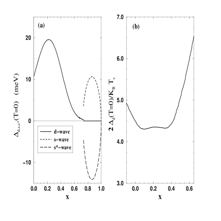
FIG. 2.: (a) Gaps $\Delta_{d,s,s^{*}}$; (b) ratio $2\Delta_{d}/K_{B}T_{c}$ as a function of doping x.

The doping dependence of the zero temperature gaps is plotted in Fig. 2 (a). The amplitude of the $d$-wave gap is always larger close at half-filling and vanishes at about x=0.7. The maximum occurs at x=0.22 irrespective of the values of the coupling constants due to fact that the Fermi level crosses over a van Hove singularity. Interestingly enough, there are $s$-wave solutions of the saddle point equations for large doping concentrations even though the on site interaction is repulsive. The $s$-wave gaps peak at $x\simeq 0.8$ because the Fermi level crosses a second van Hove singularity.

The ratio $2\,\Delta_{d}/K_{B}\,T_{c}$ (Fig. 2 (b)) has a constant value of 4.3 for doping concentrations ranging from x=0.05 to 0.4 (the ratio for a parabolic band is universal and equal to 4.25.) The highest value of $T_{c}$ therefore occurs at x=0.22, which is defined at the optimal doping concentration of this model. The ratio increases steeply for larger x, reaching a value of 7 when x is 0.67. Hence, the doping dependence of the critical temperature resembles the universal curve $T_{c}(x)$ of the cuprates.[23, 29, 30] Moreover, all physical magnitudes are expressed in real units, so that one may compare with experiments easily. The agreement doesn’t extend too far though, as the experimental doping dependence of the zero temperature gap is a monotonically decreasing function of x. [17, 31] The experimental ratio $2\Delta_{d}(T=0)/K_{B}\,T_{c}$ is therefore non constant.

plots

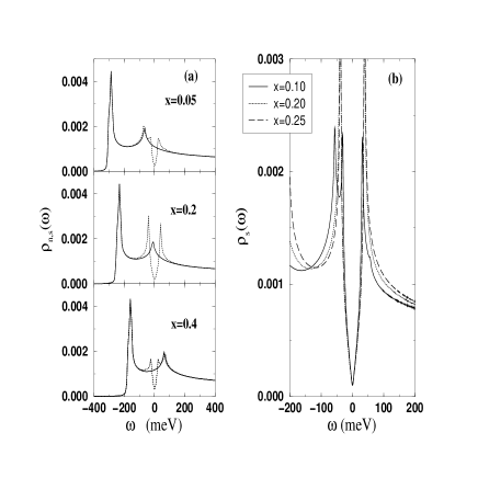
FIG. 3.: (a) Normal $\rho_{n}(\omega)$ and superconducting $\rho_{s}(\omega)$ densities of states for three doping concentrations in a frequency range which covers almost all the band; (b) superconducting density of states $\rho_{s}(\omega)$ for various x in the narrow frequency range [-200,200] meV.

For underdoped cuprates there appears another characteristic temperature $T^{*}$, which is a linearly decreasing function of the doping concentration. Above $T_{c}$ but below $T^{*}$, the $d$-wave gap partially closes down in such a way that the Fermi contour exists only in segments around the diagonals of the two-dimensional Brillouin zone. [17] Assuming that both $T^{*}$ and $\Delta_{d}(T=0)$ vanish at a doping concentration of about 0.3, the dependence of both magnitudes with x is close to a straight line of slope $p_{T,\Delta}$. A possible generalization of $2\Delta/K_{B}\,T_{c}$ for the cuprates could therefore be the ratio $2*p_{\Delta}/p_{T}$, which is approximately constant and equal to about 5.5.

The main source of trouble probably comes from the simple form of the dispersion relation of the model, where several drastic assumptions about the existence and nature of the hypothetical quasiparticles have been made: (a) There exists a well defined Fermi surface, even though this system has a pseudo gap above $T_{c}$. (b) Quasiparticles not only exist and are infinitely long-lived, but also their weight on the renormalized electronic propagator is always exactly 1. (c) The band shifts rigidly when the system is doped. To obtain the correct behavior for the doping dependence of $\Delta_{d}(T=0)$, the treatment of the dispersion relation of the fermionic degrees of freedom should be improved. In particular, if one still wishes to use a quasi-particle picture, at least assumption (b) should be relaxed.

The specific dispersion relation used gives rise to a second, weak van Hove singularity, in addition to that proper of the Hubbard t-t’ model, see Fig. 3 (a). They are responsible for the maximums attained by the zero temperature gaps as a function of doping. The dispersion relation leads to a superconducting density of states which is largely asymmetric as is also seen in a-b tunneling experiments of ${\sf Y\,Ba_{2}\,Cu_{3}\,O_{8-\delta}}$ and ${\sf Bi_{2}Sr_{2}CaCu_{2}O_{8-\delta}}$. [32, 33] Fig. 3 (b) is a plot of the density of states for three doping concentrations close to the optimal value x=0.22, in the restricted frequency range which is often used in those tunneling experiments.

TABLE II.: Changes in the gaps for $V_{0}=-250$ meV, $V_{1}=150$ meV and $x=0.2$.

$\alpha$	$\beta$	$\Delta_{d}(meV)$	$\Delta_{s}(meV)$	$\Delta_{s*}(meV)$
$0.$	$0.$	$22.1$	$0.$	$0.$
$0.05$	$0.$	$20.5$	$-0.28$	$0.57$
$0.$	$0.05$	$22.1$	$-0.23$	$1.54$
$0.05$	$0.05$	$20.6$	$-0.5$	$2.01$
$-0.05$	$0.05$	$20.4$	$0.07$	$0.86$
$0.05$	$-0.05$	$20.4$	$-0.07$	$-0.86$
$-0.05$	$-0.05$	$20.6$	$0.5$	$-2.01$

The main effect of an orthorhombic distortion of the square lattice is to allow mixing of the d and $s$-wave states, as discussed above. Such an effect can indeed be seen in the numerical solution of the saddle point equations, as shown in Table II. Another effects are related to the different role performed by the parameters $\alpha$ and $\beta$. A finite $\alpha$ also reduces the value of the $d$-wave gap. On the other hand, a finite $\beta$ doesn’t alter the $d$-wave gap so much, but induces more appreciable $s$-wave components. The relative phase between $s$ and $d$-wave gaps on two different twin domains can also be modeled by changing the sign of $\alpha$ and $\beta$ as shown in the last four rows of table II. [34]

The mapping of the tight-binding model onto a linearized Hamiltonian works quite well. There are three parameters which appear naturally in the analytic calculation, $k_{F}\,\lambda$, g, and $E_{d}$. All of them are needed to fit $\Delta_{s,d}^{L}$ onto their partners, $\Delta_{s,d}$ along the axes. The values extracted for $k_{F}\,\lambda/\pi$, g, and $E_{d}$ range from 1.21 to 1.27, 1.1 to 1.6 $eV^{-1}$, and 205 to 480 meV, respectively.[10] There are no further parameters at hand so the mapping for the remaining part of the phase diagrams can be regarded as parameter free. Fig. 1 shows that the qualitative trends are indeed captured even though the slopes of the different phase boundaries are not exactly the same.

Inclusion of superflow

The Ginsburg-Landau free energy functional of a pure $d$-wave superconductor on a perfect square lattice with a superfluid velocity $\vec{v}_{s}=\hbar\,\vec{q}/m$, [11, 23, 35, 36]

$$f = \frac{h^{2}}{8\,\pi}$$ (65)

$$+\frac{|\alpha|^{2}}{2\,\beta}\left[-\frac{1}{2}+\frac{1}{2}(|d|-1)^{2}-\xi_{s}^{2}\,|(-i\,\vec{\nabla}+\vec{q}-\frac{2\,e}{\hbar\,c}\vec{A})\,d|^{2}\right],$$

shows that the current density

$$\vec{\j}=-2\,e\,n_{s}(\vec{q})\,\vec{v_{s}}(\vec{q})=\frac{e\,\hbar\,|\alpha|}{m\,\L^{2}\,\beta}|d(\vec{q})|^{2}\,\vec{q}=\frac{e\,|\alpha|}{L^{2}\,\beta}\,(1-\frac{m\,v_{s}^{2}}{2\,|\alpha|})\,\vec{v}_{s}$$ (67)

is completely isotropic close to the critical temperature. Here, the order parameter $\Delta_{d}\propto\left[-|\alpha|/2\beta\right]^{1/2}\times\eta_{d,\vec{k}}\times d$ and $\xi_{s}=\left[\hbar^{2}/2m|\alpha|\right]^{1/2}$ is the superconducting coherence length.

plots

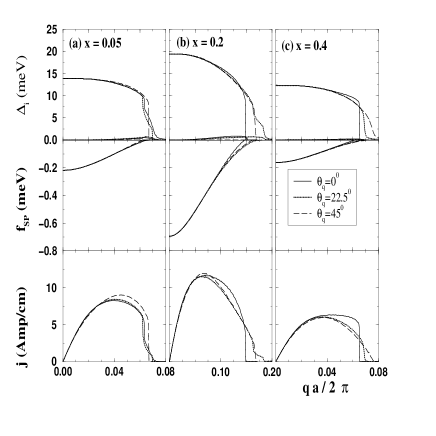
FIG. 4.: Zero Temperature gaps $\Delta_{s,s*,d}$, free energy per site $f_{SP}$, and current density ${\rm j}$ as a function of the wave vector $q$ normalized to the size of the Brillouin zone for three different angles and doping concentrations (a) x=0.05; (b) x=0.2; (c) x=0.4.

The relation between ${\rm j}$ and $q$ is linear at the beginning, but for large enough $q$, ${\rm j}$ begins to saturate and attains a maximum which defines the critical current ${\rm j}_{c}$. Afterwards, the current density decreases and eventually vanishes, although this part of the curve corresponds to metastable states and has therefore no physical relevance. The linear behavior of ${\rm j}$ for small Doppler shifts arises from the dependence of the superfluid velocity with $q$, because $n_{s}$ is then almost constant. For Doppler shifts of the order of the inverse coherence length, on the contrary, $n_{s}$ is largely depressed and so the current density saturates at a maximum which defines the critical current density ${\rm j}_{c}$.

This qualitative behavior displayed by superconductors close to $T_{c}$ is also manifested at low temperatures. The top panels of Fig. 4 show the zero temperature gaps as a function of $qa/2\pi$ for three different angles $\theta_{q}$ formed between $\vec{q}$ and the X axis, $0^{0}$, $22.5^{0}$ and $45^{0}$. The most distinct feature is that the $d$-wave gap follows very similar trends for all the angles, showing that the superflow state is indeed rather isotropic. Besides, the gaps (a) decrease slowly as they would in the Ginsburg-Landau regime, but then drop abruptly at a large $q$ value and, finally, there is sometimes a strange tail; (b) small $s$ and $s^{*}$ components are induced and grow slowly with $q$; (c) the range of $q$-values over which the gaps are finite is clearly larger for the nearly optimal doping concentration x=0.2; (d) the $d$-wave gap is somewhat smaller for $\theta_{q}=0^{0}$ than for $\theta_{q}=22,5^{0},45^{0}$, but extends to larger values of $q$ for x=0.05; on the contrary, it is bigger for the other two doping concentrations, but drops to zero earlier.

plots

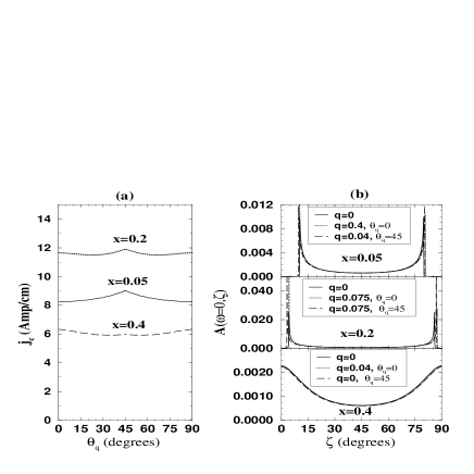
FIG. 5.: (a) Critical current density ${\rm j}_{c}$ as a function of the angle $\theta_{q}$ for three doping concentrations; (b) Angular spectral function $A(\omega=0,\zeta)$ for various values of $q$ and $\theta_{q}$. Top panel, x=0.05, middle panel, x=0.2; bottom panel, x=0.4.

The free energy is shown in the center panels. It is much the same for all angles at each doping concentration and does not show any strange feature. The bottom panels show the current densities. They display the Ginsburg-Landau behavior in a loose sense, but there are again tails at the far right range of $q$. The overall form of the curves is fairly similar again for all the angles displayed. Moreover, the superfluid density, which is the initial slope of the curve, seems to be the same for all of them. The form of the curves is markedly different for the different doping concentrations, and the current densities attained are larger again for x=0.2.

plots

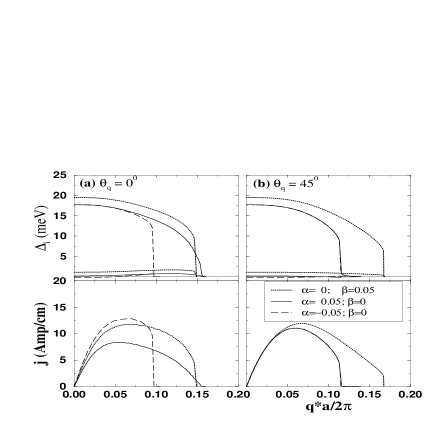
FIG. 6.: Zero Temperature gaps $\Delta_{s,s*,d}$, and current density ${\rm j}$ as a function of the wave vector $q$ normalized to the size of the Brillouin zone, for three possible values of the orthorhombic parameters $\alpha$ and $\beta$ and a doping concentration of x=0.2. The angles are (a) $\theta_{q}=0^{0}$ and (b) $\theta_{q}=45^{0}$.

The critical currents depend only slightly on the angle $\theta_{q}$, as shown in Fig. 5 (a) for several doping concentrations. A closer look reveals that ${\rm j}_{c}$ is maximum at $\theta_{q}=45^{0}$ and minimum at $\theta_{q}=0^{0}$ for x=0.05; it is still maximum at 45 degrees at x=0.2, but in this case ${\rm j}_{c}$ is a non-monotonic function of the angle; the maximum is attained at $\theta_{q}=0^{0}$ for x=0.4. This behavior can be understood in terms of the angular spectral function

$$A(\omega,\zeta<45^{0})=\int_{0}^{\pi/\cos\zeta}\,\frac{dk}{2\,\pi}\,k\,\delta(\omega-\xi(k,\zeta)),$$ (68)

which weights the back-flow term due to quasiparticles in Eq. (51). $A(\omega=0,\zeta)$ (Fig. 5 (b)) has strong peaks for small angles when x=0.05 and 0.2 and therefore the back-flow contribution to the current must then be important. $A(\omega=0,\zeta)$ is smoother for x=0.4, and accordingly, ${\rm j}_{c}$ is flatter. Indeed, the angular dependence of the critical current ${\rm j}_{c}$ is even weaker for the linearized model; ${\rm j}_{c}$ is always minimum at $\theta_{q}=45^{0}$ in such a case. Taken together, all these facts clearly indicate that the anisotropy of the band is a more efficient source of anisotropy than the internal structure of the order parameter.

The critical currents achieved are of the order of 10 Amp/cm. This leads to an estimated critical current for ${\sf Bi_{2}Sr_{2}CaCu_{2}O_{8-\delta}}$ of $5\times 10^{7}\,{\rm Amp/cm^{2}}$, which is one order of magnitude larger than the value $10^{6}\,{\rm Amp/cm^{2}}$ found in thin films some time ago.[37] Similarly, we obtain ${\rm j}_{c}\simeq 2\times 10^{8}\,{\rm Amp/cm^{2}}$ for ${\sf YBa_{2}Cu_{3}O_{8-\delta}}$, while the experimental values are of the order of $5\times 10^{7}\,{\rm Amp/cm^{2}}$, not far away.[37]

The superfluid density tensor

$$n_{s,i,j}=m\,\int_{\pi}^{\pi}\,\frac{d\vec{k}}{(2\,\pi)^{2}}\,|v_{\vec{k}}|^{2}\tanh\left(\frac{\beta\,E_{\vec{k}}}{2}\right)\,\left[M^{-1}\right]_{ij}$$ (69)

is not proportional to $|\Delta|^{2}$ as happens in Ginsburg-Landau theory.

Orthorhombic effects modeled by the $\beta$ parameter do not affect the behavior of the $d$-wave gap or the current densities. They only induce a rather large $s$ component, which also increases with $q$. The curves for $\Delta_{d}$ and ${\rm j}$ are indeed indistinguishable from those at $\beta=0$. The impact of the other orthorhombic parameter $\alpha$ is bigger. Fig. 6 shows the gaps and current densities for two opposite orthorhombic elongations of the X and Y axes, $\alpha=\pm 0.05$. For an angle $\theta_{q}=0^{0}$, (a) the $d$-wave gaps are initially reduced by the same magnitude as they should, but as $q$ increases the solution for negative $\alpha$ drops to zero faster; (b) the $s$-wave gaps have initially the same magnitude and opposite signs, but that corresponding to $\alpha=-0.05$ goes through zero, changes its sign and eventually drops to zero again; (c) the current densities show the opposite trend, in the sense that both the superfluid density $n_{s}$ and the critical current ${\rm j}_{c}$ are larger for negative $\alpha$. Moreover, superfluid densities and critical currents for $\alpha=0.05$ are even smaller than those corresponding to no orthorhombic distortion.

Fig. 6 (b) corresponds to $\theta_{q}=45^{0}$. In this case, the two orthorhombic distortions corresponding to $\alpha=\pm 0.05$ are equivalent and the curves for the $d$-wave gaps fall one on top of the other. The two $s$-wave gaps have exactly the same magnitude and different sign. The current densities are also equal as they should. The overall trend is that a finite $\alpha$ reduces both the $d$-wave gap and the critical current, although the superfluid density does not change much.

Comparison of Figs. 6 (a) and (b) shows that orthorhombicity is also a more efficient source of anisotropy that the internal symmetry of the order parameter function. Indeed, not only ${\rm j}_{c}$ but also $n_{s}$ strongly depend on $\theta_{q}$ even for these small values of the parameter $\alpha$.

plots

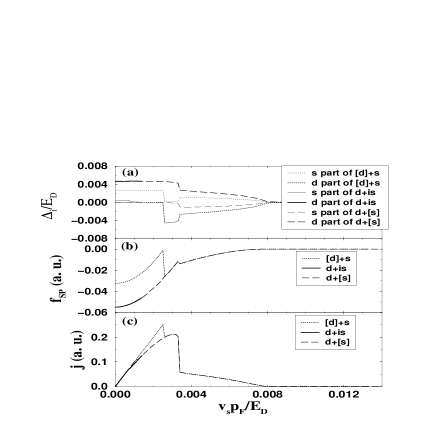
FIG. 7.: (a) Zero temperature gaps $\Delta_{i}$, (b) free energy $f_{SP}$, and (c) current density ${\rm j}$ in arbitrary units as a function of the normalized superfluid velocity in the linearized model for $\theta_{q}=0^{0}$ and $V_{s}^{L}\,{\rm g}^{L}=0.15,\,V_{d}^{L}\,{\rm g}^{L}=0.32$; $d+[s]$ and $[d]+s$ indicate mixed states with dominant $d$ or $s$ components, respectively.

The time-reversal-symmetry broken solution $d+i(s+s^{*})$ to the saddle point equations appears for attractive $V_{0}$ around the phase boundary between the $d$ and $s+s^{*}$ solutions. In this part of the phase diagram, there exist not only the $d+i(s+s^{*})$ state, but also finite $s+s^{*}$ and d solutions. The phase transitions from one stable state to another are therefore first order. A finite Doppler shift gives rise to (a) mixing between the d and $s+s^{*}$ states so that each of these two solutions is of the form $s+s^{*}+[d]$ or $[s+s^{*}]+d$; where the subdominant component is enclosed in brackets; (b) competition between these two solutions and with the broken time-reversal-symmetry state.

Numerical calculations for the linearized case and suitably chosen values of $V_{s}^{L}$ and $V_{d}^{L}$ are displayed in Figs. 7 and 8 for angles $\theta_{q}=0^{0}$ and $45^{0}$. They show that the $d+is$ state is initially more stable but the s component decreases when $v_{s}$ increases and eventually vanishes. The $d+is$ state disappears at that moment in favor of the $d+[s]$ state, $[d]+s$ being higher in energy. The $d+[s]$ solution becomes metastable once the critical current density of that state is reached. There is then a phase transition to the $[d]+s$ state, which has a higher ${\rm j}_{c}$, because it is the current what is actually imposed in an experimental setup. Above this second critical current density, the system reverts to its normal phase.

plots

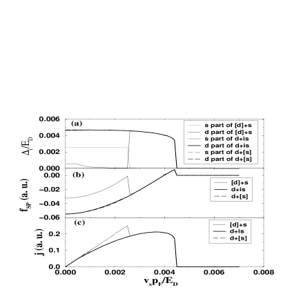
FIG. 8.: (a) Zero temperature gaps $\Delta_{i}$, (b) free energy $f_{SP}$ ,and (c) current density ${\rm j}$ in arbitrary units as a function of the normalized superfluid velocity in the linearized model for $\theta_{q}=45^{0}$ and $V_{s}^{L}\,{\rm g}^{L}=0.15,\,V_{d}^{L}\,{\rm g}^{L}=0.32$.

Conclusions

The formalism needed to include superflow in a gauge invariant way in a superconductor has been discussed in detail and shown to be equivalent to give a Doppler shift to the wave vectors in the kinetic energy part of the Hamiltonian. This has been applied to study supercurrents in a clean, infinite, $d$-wave superconductor on an orthorhombically distorted square lattice, using a model which describes some of the features of the superconducting state of several High-temperature superconductors. The behavior of gaps, free energy, current density and critical current as a function of modulus and angle of the Doppler shift, doping, and orthorhombic distortion have been discussed.

There are three possible sources of anisotropy in the discussed model: the internal symmetry of the order parameter, the complex dispersion relation of the band and the orthorhombic distortion of the lattice. The results of this article show that the most important one is orthorhombicity distortion, then the form of the band and last and least the $d$-wave form of the gap function.

After this work was completed we found that D. Feder and C. Kallin had also been studying the behavior of supercurrents in $d$-wave superconductors and had reached conclusions which agree with those of this article.

- [1] J. R. Reitz, F. J. Milford, and R. W. Christy, Foundations of Electromagnetic Theory (Addison-Wesley, Reading, Massachussets, 1979).
- [2] D. S. Pyun, E. R. Ulm, and T. R. Lemberger, Phys. Rev. B 39, 4140 (1989).
- [3] J. R. Schrieffer, Theory of superconductivity (Addison-Wesley, Reading, Massachussets, 1964).
- [4] J. Ferrer, Ph.D. thesis, Universidad Autónoma de Madrid, 1990.
- [5] A. Furusaki and M. Tsukada, Solid State Commun. 78, 299 (1991).
- [6] Y. B. Kim and M. J. Stephen, in Superconductivity, vol. II, edited by R. D. Parks (Dekker, New York, 1969).
- [7] D. S. Dessau et al., Phys. Rev. Lett. 71, 2781 (1993).
- [8] K. Gofron et al., Phys. Rev. Lett. 73, 3302 (1994).
- [9] M. R. Norman, M. Randeria, H. Ding, and J. C. Campuzano, Phys. Rev. B 52, 615 (1995).
- [10] J. Ferrer, M. A. González-Alvarez, and J. Sánchez-Cañizares, Phys. Rev. B 57, 7470 (1998).
- [11] M. Zapotocky, D. Maslov, and P. M. Goldbart, Phys. Rev. B 55, 6599 (1997).
- [12] K. Maki, in Superconductivity, vol. II, edited by R. D. Parks (Dekker, New York, 1969).
- [13] P. Bagwell, Phys. Rev. B 49, 6841 (1994).
- [14] J. Sánchez-Cañizares and F. Sols, Phys. Rev. B 55, 531 (1997).
- [15] A. Martin and C. J. Lambert, Phys. Rev. B 51, 17999 (1995).
- [16] A. van Otterlo, D. S. Golubev, A. D. Zaikin, and G. Blatter, condmat/9703124 (unpublished) .
- [17] H. Ding et al., condmat/9712100 (unpublished) .
- [18] D. J. Scalapino, Physics Reports 250, 330 (1995).
- [19] A. V. Chubukov, D. Pines, and B. P. Stojkovic, J. Phys. Condens. Matter 8, 10017 (96).
- [20] J. Annett, N. Goldenfeld, and A. J. Leggett, in Physical Properties of High Temperature superconductors V, edited by D. M. Ginsberg (World Scientific, New Jersey, 1996).
- [21] R. Micnas, J. Ranninger, and S. Robaszkiewicz, Rev. Mod. Phys. 62, 113 (1990).
- [22] A. Nazarenko, A. Moreo, E. Dagotto, and J. Riera, Phys. Rev. B 54, R768 (1996).
- [23] D. L. Feder and C. Kallin, Phys. Rev. B 55, 559 (1997).
- [24] M. T. Beal-Monod and K. Maki, Phys. Rev. B 53, 5775 (1996).
- [25] K. A. Musaelian, J. Betouras, A. V. Chubukov, and R. Joynt, condmat/9507085 (unpublished) .
- [26] C. O’Donovan and J. P. Carbotte, condmat/9502035 (unpublished) .
- [27] P. Chandra and B. Douçot, Phys. Rev. B 38, 9335 (1988).
- [28] J. Ferrer, Phys. Rev. B 47, 8769 (1993).
- [29] D. Duffy et al., Phys. Rev. B 56, 5597 (1997).
- [30] P. N. Spathis, M. P. Soerensen, and N. Lazarides, Phys. Rev. B 45, 7360 (1992).
- [31] N. Miyakawa et al., Phys. Rev. Lett. 80, 157 (1998).
- [32] Y. DeWilde et al., Phys. Rev. Lett. 80, 153 (1998).
- [33] Ch. Renner et al., Phys. Rev. Lett. 80, 149 (1998).
- [34] K. A. Kouznetsov et al., Phys. Rev. Lett. 79, 3050 (1997).
- [35] R. Joynt, Phys. Rev. B 41, 4271 (1990).
- [36] Y. Ren, J.H. Xu, and C. S. Ting, Phys. Rev. Lett. 74, 3680 (1995).
- [37] T. R. Lemberger, in Physical Properties of High Temperature superconductors III, edited by D. M. Ginsberg (World Scientific, New Jersey, 1992).