Non-Fermi liquid regime of a doped Mott insulator

Abstract

We study the doping of a Mott insulator in the presence of quenched frustrating disorder in the magnitude and sign of the magnetic exchange. Two quite different doping regimes $\delta<\delta^{*}$ and $\delta>\delta^{*}$ are found, with $\delta^{*}\simeq J/t$ ($J$ is the characteristic magnitude of the exchange, and $t$ the hopping amplitude). In the high-doping regime, a (Brinkman-Rice) Fermi liquid description applies with a coherence scale of order $\delta t$. In the low doping regime, local magnetic correlations strongly affect the formation of quasiparticles, resulting in a very low coherence scale $\epsilon_{F}^{*}\simeq J(\delta/\delta^{*})^{2}$. Fermi liquid behaviour does apply below $\epsilon_{F}^{*}$, but a “quantum critical regime” $\epsilon_{F}^{*}<T<J$ holds, in which marginal Fermi liquid behaviour of several physical properties is found: NMR relaxation time $1/T_{1}\sim\mbox{const.}$, resistivity $\rho_{dc}(T)\propto T$, optical lifetime $\tau_{opt}^{-1}\propto\omega/\ln(\omega/\epsilon_{F}^{*})$ together with $\omega/T$ scaling of response functions, e.g. $J\sum_{\vec{q}}\chi^{\prime\prime}(\vec{q},\omega)\propto\tanh(\omega/2T)$. In contrast, single-electron properties display stronger deviations from Fermi liquid theory in this regime with a $\sqrt{\omega}$ dependence of the inverse single-particle lifetime and a $1/\sqrt{\omega}$ decay of the photoemission intensity.

On the basis of this model and of various experimental evidence, it is argued that the proximity of a quantum critical point separating a glassy Mott-Anderson insulator from a metallic ground-state is an important ingredient in the physics of the normal state of cuprate superconductors. In this picture the corresponding quantum critical regime is a “slushy” state of spins and holes with slow spin and charge dynamics responsible for the anomalous properties of the normal state. This picture may be particularly relevant to $Zn-$doped materials.

I Introduction

How (and whether) coherent quasiparticles form in a lightly doped Mott insulator is a key question in the physics of strongly correlated electron systems. A satisfactory theoretical understanding of this issue has been achieved in the limit where magnetic correlations do not play a prominent role, starting with the work of Brinkman and Rice [1, 2, 3]. In cuprate superconductors however, the undoped phase is an antiferromagnetic insulator with a rather large exchange coupling $J_{AF}$ (on the scale of $100\,meV$), so that we have to face the problem of the interplay between local coherence and magnetic correlations.

Furthermore, there is ample experimental evidence that carrier localisation and magnetic frustration also play a crucial role in the low to intermediate doping regime. This is particularly clear in the $\mbox{La}_{2-x}\mbox{Sr}_{x}\mbox{Cu}\mbox{O}_{4}$ compound at concentrations just above $x=0.02$ (the threshold for the disappearance of the antiferromagnetic long-range order), for which true spin-glass ordering of the copper moments has been demonstrated at very low temperature (with $T_{g}\simeq 7K$ for $x=0.04$ [4]). Up to which doping concentration does this glassy regime persist when superconductivity is suppressed is not known at this point, but carrier localization is indeed observed at low temperature up to optimal doping in both the $ab$ and $c$ directions when a strong magnetic field is applied [5, 6]. It was actually predicted early on [7] that hole doping induces strong frustration in the system when the holes become localized, replacing locally an antiferromagnetic Cu-Cu bond with an effectively ferromagnetic one, with a strength larger than the original $J_{AF}$. We observe furthermore that the disappearance of antiferromagnetic long-range order is accompanied by the appearance of new low-energy spin excitations, of a quite different nature than spin waves, as evidenced by inelastic neutron scattering experiments [8]-[15]. It is important to notice that the compounds with a glassy ground-state display, at sufficiently high temperature (above the onset of localization), the same distinctive transport properties as in samples with higher doping, e.g. linear resistivity [8, 10]. It is thus tempting to view these low-energy excitations as the source of anomalous scattering in the normal state.

Anticipating some of the speculations made at the end of this paper, we shall argue that these low energy excitations are associated with a novel kind of spin state: the “slushy” state associated with the disordering of an insulating (possibly glassy) ground state by hole motion, quantum fluctuations and thermal effects. In this picture, many distinctive “anomalous” properties of the normal state of the cuprate superconductors are associated with the quantum critical regime corresponding to the $T=0$ transition at which the insulating (glassy) ground-state melts into a metallic (Fermi-liquid) ground state when doping is increased.

In this paper, we shall study a highly simplified model of such a slushy state of spins and holes. Our starting point is the work of Sachdev and Ye [17], who showed that in the large-$M$ limit of the fully-connected random Heisenberg model of $SU(M)$ spins, quantum fluctuations are strong enough to overcome the tendency to spin-glass ordering. Instead, a gapless spin-liquid state is found down to zero temperature with a large density of low-energy spin excitations [18]. Remarkably, these excitations are characterized by a local dynamic spin susceptibility which has precisely the form advocated by the “marginal Fermi liquid” phenomenological description [19] of the low energy spin excitations in cuprates, namely:

$$\chi_{loc}^{\prime\prime}(\omega,T=0)={{\pi}\over{2J}}\mbox{sgn}(\omega)\,\,\,,\,\,\,\chi_{loc}^{\prime}(\omega,T=0)={{\sqrt{\pi}}\over{2J}}\ln\left({{J}\over{|\omega|}}\right)$$ (1)

This model is one of the few cases in which a response function having the marginal Fermi liquid form could be derived explicitly (see also [20]). The generalization of Eq.(1) to finite temperature will be given in Sec.III C (Eq. (70)) and displays $\omega/T$ scaling. The physical mechanism for the gaplessness and the high-density of spin excitations in this model is discussed in more detail at the beginning of Sec.III. It has to do with the large number of transverse components of the spins in the large-$M$ limit. In this respect, it might be a reasonable picture for the disordering of the two-dimensional quantum Heisenberg spin-glass due to quantum fluctuations and low dimensionality [21].

The main purpose of this paper is to determine whether this marginal Fermi liquid spectrum survives the introduction of charge carriers and the associated insulator to metal transition. The physics of this problem is dominated by the interplay between two competing effects:

• The formation of coherent metallic quasiparticles, which can be viewed as a binding of spin and charge degrees of freedom. In the simplest description of a doped Mott insulator with $U=\infty$, coherent quasiparticles form below a scale of order $T^{*}_{F0}\sim\epsilon^{*}_{F0}\sim\delta t$ (where $\delta$ is the doping and $t$ the hopping amplitude). This is a “naive” estimate of the effective Fermi-energy scale, since it ignores any effect coming from the magnetic exchange (which will tend to suppress it).

• The binding of spin degrees of freedom on neighbouring sites into singlet or triplet states, and the corresponding slow dynamics of the on-site local moment. This is the phenomenon leading to the formation of the spin-liquid state in the undoped phase, which involves a scale of order $J$ (the characteristic strength of the exchange).

It is clear from comparing the scales above that when $J$ is larger than the “naive” coherence scale $\epsilon^{*}_{F0}$, the magnetic exchange prevents the formation of coherent quasiparticles at that scale: in other words, $\epsilon^{*}_{F0}$ cannot possibly be the actual quasiparticle coherence scale above which free local moments are recovered, since the exchange is still effective at energy scales between $\epsilon^{*}_{F0}$ and $J$. It is thus expected that the actual coherence scale of the system, $\epsilon^{*}_{F}$ will be much smaller than $\epsilon^{*}_{F0}$, and that a new metallic regime in which spin degrees of freedom form a spin-liquid like state while charge degrees of freedom are incoherent will be found in the intermediate energy and temperature range $\epsilon^{*}_{F}<\omega,T<J$. From the above estimates, this will be the case at small doping: $\delta<\delta^{*}\sim J/t$, while a direct crossover from a coherent metal to an incoherent high temperature state is expected for $\delta>\delta^{*}$. These expectations are entirely borne out from our solution of the doped Sachdev-Ye model, as evidenced by Fig.1, which summarizes the main crossovers found in our analysis.

It should be emphasized that this competition between metallic coherence and magnetic exchange is also essential to the physics of heavy fermion compounds [22]. In this context, the “naive” coherence scale $\epsilon^{*}_{F0}$ stands for the single-impurity Kondo scale (or rather, any estimate of the lattice Kondo scale that ignores RKKY interactions), while $J$ stands for the typical strength of the RKKY interaction. For this reason, the results of the present paper may also have some relevance, with appropriate changes, to the physics of the disordered rare-earth compounds near the quantum critical transition into a spin glass ground state [23].

II The Model

A Disordered $SU(M)$ $t-J$ model

The effect of charge carriers on the Sachdev-Ye spin-liquid phase will be investigated by generalizing the model of Ref. [17] to a $t-J$ model, with randomness on the exchange couplings $J_{ij}$ between nearest neighbors sites :

$$H=-\sum_{<ij>\alpha}t_{ij}\,P\,c^{\dagger}_{i\alpha}c_{j\alpha}\,P+\sum_{<ij>}J_{ij}\vec{S}_{i}\cdot\vec{S}_{j}$$ (2)

In this expression, the $SU(2)$ spin symmetry of the electrons has been enlarged to $SU(M)$ [25]. $\vec{S}_{i}$ is the conduction electron spin density on site $i$ and the spin index $\alpha$ runs over $\alpha=1,\cdots,M$. The projection operator $P$ enforces the local constraint:

$$\sum_{\alpha}c^{\dagger}_{i\alpha}c_{i\alpha}\leq\frac{M}{2}$$ (3)

In this manner the $M=2$ case exactly coincides with the standard $t-J$ model with the constraint of no double occupancy.

The exchange couplings are quenched random variables with random sign and magnitude, distributed according to a Gaussian distribution with :

$$J_{ij}={J\over\sqrt{zM}}\epsilon_{ij}\,\,\,,\,\,\,\overline{\epsilon_{ij}}=0\,\,\,,\,\,\,\overline{\epsilon_{ij}^{2}}=1$$ (4)

(throughout this paper the bar will denote an average over the disorder). In the following, we shall consider this model on a lattice of connectivity $z$, with a nearest-neighbor hopping amplitude normalized as:

$$t_{ij}={{2t}\over{M\sqrt{z}}}$$ (5)

and we shall analyze the model in the following double limit:

• $z\rightarrow\infty$. In this limit of infinite connectivity, a dynamical mean field theory applies which reduces the model to the study of a single-site self-consistent problem [3], as detailed in Sec. II B. However this single site model is still a complicated interacting problem. For the sake of simplicity, the lattice will be taken to be a Bethe lattice (no essential physics is lost in this assumption).

• $M\rightarrow\infty$, in which the single site problem becomes tractable. In the absence of a random exchange, this limit yields the familiar Brinkman-Rice description of a doped Mott insulator [1, 25].

The scaling in $z$ and $M$ in (4) and (5) are chosen such that this double limit gives non trivial results. Alternatively, one could consider (as in [17]) this model on a fully connected lattice of $N$ sites, with random hopping amplitudes: $t_{ij}={{2t}\over{M\sqrt{N}}}\xi_{ij}$ with $\overline{\xi_{ij}}=0$, $\overline{\xi_{ij}^{2}}=1$. This leads to precisely the same equations for single particle Green’s functions as the $z=\infty$ Bethe lattice [3].

We shall use a decomposition of the physical electron operator into a spin-carrying fermion $f$ and a slave boson $b$ : $c^{+}_{i\alpha}=f^{+}_{i\alpha}b_{i}$. The local constraint (3) becomes :

$$\sum_{\alpha}f^{\dagger}_{i\alpha}f_{i\alpha}+b^{\dagger}_{i}b_{i}={M\over 2}$$ (6)

With this decomposition the Hamiltonian (2) can be rewritten as:

$$H=-{{2t}\over{M\sqrt{z}}}\sum_{<ij>\alpha}(f^{\dagger}_{i\alpha}b_{i}b^{\dagger}_{j}f_{j\alpha}+h.c)+{{J}\over{\sqrt{Mz}}}\sum_{<ij>}\epsilon_{ij}\sum_{\alpha\beta}S_{i\alpha\beta}S_{j\beta\alpha}$$ (7)

and the $M^{2}-1$ components of the $SU(M)$ spin operators $\vec{S}_{i}=(S_{i})^{\alpha\beta}$ read :

$$S_{i\alpha\beta}=f^{+}_{i\alpha}f_{i\beta}-{{1}\over{M}}\delta_{\alpha\beta}\sum_{\alpha}f^{+}_{i\alpha}f_{i\alpha}$$ (8)

B Reduction to a single-site problem

In this section, we explain how the large connectivity limit $z\rightarrow\infty$ reduces the problem to the study of a single-site model supplemented by a self-consistency condition. First we use a path integral representation of the partition function $Z$ and introduce a Lagrange multiplier field $\lambda_{i}(\tau)$ on each site in order to handle the constraint (6). We then introduce $n$ replicas of the fields ($f_{i}^{a},b_{i}^{a},\lambda_{i}^{a}\,\,\,,a=1,\cdots,n$) in order to express $Z^{n}$ and average over the disorder. The action associated with $\overline{Z^{n}}$ reads:

$$S= \sum_{i,a}S_{0}[f^{\dagger a}_{i},f_{i}^{a},b^{\dagger a}_{i},b_{i}^{a},\lambda_{i}^{a}]-{2t\over\sqrt{z}M}\sum_{<i,j>,\alpha}\int_{0}^{\beta}d\tau f^{\dagger a}_{i\alpha}(\tau)b^{a}_{i}(\tau)b^{\dagger a}_{j}(\tau)f^{a}_{j\alpha}(\tau)$$ (10)

$$-{J^{2}\over 2zM}\int_{0}^{\beta}\!\!\!\int_{0}^{\beta}d\tau d\tau^{\prime}\,\sum_{<ij>}\sum_{1\leq\alpha,\beta,\gamma,\delta\leq M}\sum_{1\leq a,b\leq n}\,S^{a}_{i\alpha\beta}(\tau)S^{a}_{j\beta\alpha}(\tau)S^{b}_{i\gamma\delta}(\tau^{\prime})S^{b}_{j\delta\gamma}(\tau^{\prime})$$

where the action $S_{0}$ is defined by

$$S_{0}[f^{\dagger},f,b^{\dagger},b,\lambda] \equiv \int_{0}^{\beta}d\tau\left(b^{\dagger}(\tau)\partial_{\tau}b(\tau)+\sum_{\alpha}f^{\dagger}_{\alpha}(\tau)(\partial_{\tau}-\mu)f_{\alpha}(\tau)\right)$$ (12)

$$+i\int_{0}^{\beta}d\tau\lambda(\tau)\left(\sum_{\alpha}f^{\dagger}_{\alpha}(\tau)f_{\alpha}(\tau)+b^{\dagger}(\tau)b(\tau)-\frac{M}{2}\right)$$

Following the “cavity method” (reviewed in [3]), a site of the lattice is singled out, and a trace is performed over all degrees of freedom at the other sites (concentrating on phases without translational symmetry breaking, so that all sites are equivalent). In the $z\rightarrow\infty$ limit, this can be performed explicitly, and the problem reduces to a single-site effective action which reads:

$$S_{eff}= \sum_{a}S_{0}[f^{\dagger a},f^{a},b^{\dagger a},b^{a},\lambda^{a}]-{J^{2}\over 2M}\sum_{a,b,\alpha,\beta,\gamma,\delta}\int_{0}^{\beta}\!\!\!\int_{0}^{\beta}d\tau d\tau^{\prime}\,S^{a}_{\alpha\beta}(\tau)R^{ab}_{\beta\alpha\delta\gamma}(\tau-\tau^{\prime})S^{b}_{\gamma\delta}(\tau^{\prime})$$ (14)

$$+\left(\frac{2t}{M}\right)^{2}\sum_{a,\alpha}\int_{0}^{\beta}\!\!\!\int_{0}^{\beta}d\tau d\tau^{\prime}\,f^{\dagger a}_{\alpha}(\tau)b^{a}(\tau)C^{aa}_{\alpha\alpha}(\tau-\tau^{\prime})b^{\dagger a}(\tau^{\prime})f^{a}_{\alpha}(\tau^{\prime})$$

This effective action is supplemented by a self-consistency condition which constrains $C(\tau-\tau^{\prime})$ and $R(\tau-\tau^{\prime})$ to coincide with the local electron Green’s function and spin correlation function respectively:

$$C^{aa}_{\alpha\alpha}(\tau,\tau^{\prime}) = -{\left\langle Tc^{a}_{i\alpha}(\tau)c^{\dagger a}_{i\alpha}(\tau^{\prime})\right\rangle}_{S}=-{\left\langle T(f^{a}_{\alpha}b^{\dagger a})(\tau)(f^{\dagger a}_{\alpha}b^{a})(\tau^{\prime})\right\rangle}_{S_{eff}}$$ (15)

$$R^{ab}_{\alpha\beta\gamma\delta}(\tau,\tau^{\prime}) = {\left\langle S^{a}_{i\alpha\beta}(\tau)S^{b}_{i\gamma\delta}(\tau^{\prime})\right\rangle}_{S}={\left\langle S^{a}_{\alpha\beta}(\tau)S^{b}_{\gamma\delta}(\tau^{\prime})\right\rangle}_{S_{eff}}$$ (16)

In each of these equations, the last equality expresses the fact that local correlation functions can be calculated using the single-site action $S_{eff}$ itself. The limit $n\rightarrow 0$ must eventually be taken in these equations.

C Saddle-point equations in the large-$M$ limit and slave-boson condensation

We shall study the above self-consistent single-site problem in the large $M$ limit, focusing on the paramagnetic phase of the model. In this case, all the above correlators become replica diagonal ($C^{aa}=C$, $D^{ab}=D\delta_{ab}$).

Furthermore, we shall look for solutions in which the slave boson undergoes a Bose condensation. (Solutions with an uncondensed boson when the bosons carry an additional channel index have been investigated by Horbach and Ruckenstein [24]). The solutions considered here can be found as a saddle-point of $S_{eff}$ by setting: $b(\tau)=\sqrt{M/2}\phi(\tau)$ and looking for solutions in which both $\phi(\tau)$ and the Lagrange multiplier $\lambda(\tau)$ become static at the saddle-point:

$$b_{sp}(\tau)=\sqrt{M\over 2}\sqrt{\delta}\,\,\,,\,\,\,i\lambda_{sp}(\tau)=\lambda_{0}$$ (17)

From the constraint Eq.(6), the total number of electrons will be related to $\delta$ through: $\sum_{\alpha}<f^{\dagger}_{\alpha}f_{\alpha}>={M\over 2}(1-\delta)$ so that $\delta$ measures the number of holes doped into the system.

The saddle point equations then reduce to a non-linear integral equation for the fermion Green’s function $-<Tf_{\alpha}(\tau)f^{\dagger}_{\beta}(\tau^{\prime})>\equiv\delta_{\alpha\beta}G_{f}(\tau-\tau^{\prime})$, which reads (with : $\omega_{n}=(2n+1)\pi/\beta$ the Matsubara frequencies):

$$G^{-1}_{f}(i\omega_{n})=i\omega_{n}+\mu-\lambda_{0}-(t\delta)^{2}G_{f}(i\omega_{n})-\Sigma_{f}(i\omega_{n})$$ (19)

$$\Sigma_{f}(\tau)\equiv-J^{2}G^{2}_{f}(\tau)G_{f}(-\tau)$$ (20)

and to the following relations, which determine the Lagrange multiplier $\lambda_{0}$ and the chemical potential $\mu$ for given values of the doping $\delta$ and the temperature (given the couplings $J$ and $t$):

$$G_{f}(\tau=0^{-})=\frac{1-\delta}{2}$$ (21)

$$\lambda_{0}\sqrt{\delta}=-2t^{2}\delta^{\frac{3}{2}}\int_{0}^{\beta}\!d\tau G_{f}(\tau)G_{f}(-\tau)$$ (22)

The derivation of these saddle point equations from $S_{eff}$ is detailed in Appendix A.

The local spin-spin correlation function is directly related to $G_{f}$ in the $M\rightarrow\infty$ limit, as:

$$R(\tau)\equiv{{1}\over{M^{2}}}\sum_{\alpha\beta}<S_{i\alpha\beta}(\tau)S_{i\beta\alpha}(0)>=-G_{f}(\tau)G_{f}(-\tau)$$ (23)

In the following, we shall often consider the spectral functions associated with the single-particle Green’s function and the local spin-spin correlation:

$$\rho_{f}(\omega)\equiv-\frac{1}{\pi}\mathop{\hbox{Im}}G_{f}(\omega+i0^{+})\,\,\,,\,\,\,\chi_{loc}^{\prime\prime}(\omega)\equiv\mathop{\hbox{Im}}R(\omega+i0^{+})$$ (24)

III Physical properties of the metallic state

In this section, we study the nature of the metallic state as a function of the doping level $\delta$.

Let us first recall some of the properties of the spin-liquid insulating state found for $\delta=0$, as obtained by Sachdev and Ye [17]. In this case, our equations (19-21) coincide with those of Ref.[17]. Note that Eq.(22) decouples, being automatically satisfied at $\delta=0$, and that particle-hole symmetry imposes $\mu-\lambda_{0}=\Sigma_{f}^{\prime}(i0^{+})=0$. A low-frequency analysis of the integral equation reveals that the $T=0$ Green’s function and spectral density have a $1/\sqrt{\omega}$ singularity for $|\omega|\rightarrow 0$. More precisely [26], in the complex frequency plane as $z\rightarrow 0$:

$$G_{f}(z)=\left({{\pi}\over{4J^{2}}}\right)^{1/4}{{(1-i)}\over{\sqrt{z}}}+\cdots\,\,\,,\,\,\,\mbox{Im}z>0$$ (25)

This yields the following behaviour of the local dynamical susceptibility for $\omega\rightarrow 0$:

$$\chi_{loc}^{\prime\prime}(\omega)={{\pi^{3/2}}\over{4J}}\,\mbox{sgn}(\omega)+\cdots$$ (26)

Fig.2 displays a numerical calculation of $\rho_{f}(\omega)$ and $\chi_{loc}^{\prime\prime}(\omega)$ at zero doping (in agreement with the one in Ref.[17]). These results display the above low-frequency behaviour (but we note that significant corrections to (26) are already sizeable at rather low values of $\omega/J$.)

Hence the insulator at $\delta=0$ is a gapless quantum paramagnet (spin liquid), with a rather large density of low-energy spin excitations. Remarkably, (26) is of the same form than the “marginal Fermi liquid” susceptibility proposed on phenomenological grounds by Varma et al. [19] for the normal state of the cuprate superconductors. In the present context, the physical nature of these low-energy excitations is intimately connected to the fact that the exchange couplings $J_{ij}$ are random in sign. In constructing the ground-state of the insulator, let us imagine that we first try to satisfy the bonds with the larger exchange constants. When such a bond is antiferromagnetic, the two spins connected by it will form a non-degenerate singlet. For a ferromagnetic bond however, the two spins will pair into a state of maximal possible spin (the generalization to $SU(M)$ of a triplet state). This state has a degeneracy, which actually becomes very large (exponential in $M$) as $M$ becomes large. Continuing the process in order to accommodate bonds with smaller strengths will tend to remove part of this degeneracy [27], but leaves behind a very large density of low-energy spin excitations. These effects are clearly favored by the (fermionic) large-$M$ limit considered here, because of the high degeneracies of the “triplet” state and because the strength of quantum fluctuations in this limit precludes the appearance of long-range order (e.g. spin-glass) which would remove degeneracies in a different manner. We believe however that this physics is not an artefact of the large$-M$ limit. Indeed, preliminary theoretical studies [28] suggest that the local spin correlations near the quantum critical point associated with the $T=0$ transition into a metallic spin-glass phase could be similar to Eq.(26), with a related physics.

Finally, we note that the single-site action to which the model reduces at zero doping (i.e Eq. (14) with $t=0$) has some similarities with the multichannel Kondo effect in the overscreened case. In the present context however, the “bath” seen by the spin is not due to an electronic conduction band, but generated by all the other spins in the lattice. The spin correlations of both the bath and the spin adjust to the self-consistent long-time behaviour: $<S(0)S(\tau)>\sim R(\tau)\sim 1/\tau$ similar to that of the $SU(M)$ Kondo model with $K=M$ channels [30] (2-channel model in the $SU(2)$ case).

A Low-frequency analysis and the Fermi liquid coherence scale

The first question we would like to address is whether the “marginal Fermi liquid” spin dynamics survives the introduction of charge carriers. As we shall demonstrate, this depends on the temperature range considered (Fig.1). At low temperature, below some -possibly very low- coherence scale $\epsilon_{F}^{*}$, it turns out that a Fermi liquid is recovered.

This is easily seen from a low-frequency analysis of the integral equation for $G_{f}$ at zero-temperature. At zero doping, the Green’s function and self-energy behave at low-frequency as: $G_{f}(\omega)\sim 1/\sqrt{J\omega}\,\,,\,\,\Sigma_{f}(\omega)\sim\sqrt{J\omega}$. When inserted in Eq.(19), this controls the leading low-frequency behaviour of both the r.h.s and l.h.s of the equation taken at $\delta=0$, which match each other. However, for $\delta\neq 0$, the term $(t\delta)^{2}G_{f}(\omega)$ would introduce a $1/\sqrt{\omega}$ singularity and prevent this matching from taking place: this indicates that the low-frequency behaviour of the zero-temperature Green’s function for arbitrary small doping is no longer $1/\sqrt{\omega}$. In this respect, an infinitesimal doping is a singular perturbation of the above equations. This observation directly yields an estimate of the coherence scale $\epsilon_{F}^{*}$ such that $G_{f}(\omega)\sim 1/\sqrt{\omega}$ is recovered for $\epsilon_{F}^{*}<\omega\ll J$. Indeed, the term $(t\delta)^{2}G_{f}(\omega)$ becomes comparable to $\Sigma_{f}(\omega)$ in this regime (thus providing a cut-off to the singular behaviour) when $\omega\simeq(\delta t)^{2}/J$. Hence, in the low-doping regime:

$$\epsilon_{F}^{*}={{(\delta t)^{2}}\over{J}}\,\,\,,\,\,\,(\delta\ll\delta^{*})$$ (27)

where $\delta^{*}$ will be precised below. (In the following we shall take Eq.(27) as defining $\epsilon_{F}^{*}$ in the low-doping regime, with no additional prefactors).

In the high-doping regime on the other hand (or when $t\gg J$), one should consider first the limit of a vanishing magnetic exchange $J=0$. In this limit, the usual slave-boson (large $M$) description of a doped Mott insulator is recovered [2]. Setting $J=\Sigma_{f}=0$ in the equations above yields a semi-circular spectral density:

$$\rho_{f}^{J=0}=\frac{1}{\delta}D\left(\frac{\omega+\mu-\lambda_{0}}{\delta}\right)$$ (28)

where $D$ is given by :

$$D(\epsilon)=\frac{1}{\pi t}\sqrt{1-\left(\frac{\epsilon}{2t}\right)^{2}}$$ (29)

The original bandwith $4t$ of the non-interacting case has been reduced by a factor $\delta$, and the usual Brinkman-Rice result for the coherence scale is recovered :

$$\epsilon_{F}^{*}=t\delta\,\,\,,\,\,\,(\delta\gg\delta^{*})$$ (30)

Turning on $J$ as a perturbation from this starting point does not affect the leading low-frequency behaviour of the self-energy, but does lead to a scattering rate $\mathop{\hbox{Im}}\Sigma_{f}\propto\omega^{2}J^{2}/(\delta t)^{3}+\cdots$ characteristic of a Fermi liquid (in contrast the $J=0$ model has infinite quasiparticle lifetime in the large-$M$ limit). From Eqs.(30,27), it is clear that when the magnetic scattering is strong ($J\gg t$), regime (27) always applies, while for weaker scattering ($J<t$) a crossover between the two regimes is found at a characteristic doping:

$$\delta^{*}\sim\mbox{min}({{J}\over t},1)$$ (31)

We thus observe that below some characteristic doping the low-energy coherence scale is strongly affected by the magnetic scattering. When the exchange is large or for doping smaller that $\delta^{*}\simeq J/t$, the actual coherence scale $\epsilon_{F}^{*}$ is much smaller than the “naive” coherence scale $\epsilon^{*}_{F0}$ (which holds in the absence of magnetic correlations). Here we find $\epsilon^{*}_{F0}\simeq\delta t$ and $\epsilon_{F}^{*}/\epsilon^{*}_{F0}\simeq\delta/\delta^{*}$. This is one of the crucial physical conclusions of this paper.

A numerical solution of the saddle-point equations provide a clear evidence for these two regimes. The numerical procedure that we have used is explained in Appendix C. Fig. (3) displays the $T=0$ spectral function $\rho_{f}(\omega)$ for three values of $J$. When $J$ is very small, the spectral function is very close to the semi-circular shape (28), while for a larger $J$ the $1\over\sqrt{\omega}$ divergence is observed over a large frequency range $\epsilon_{F}^{*}<\omega<J$ but is cutoff for $\omega<\epsilon_{F}^{*}$ so that $\rho_{f}(0)$ is finite. Anticipating on the results of Sec. III B, we observe that the value of $\rho_{f}(\omega=0,T=0)$ is actually independent of $J$ as a consequence of the Luttinger theorem. Indeed, the following relation can be established at zero-temperature:

$$\mu-\lambda_{0}-\Sigma_{f}(i0^{+})\rightarrow\delta\mu_{0}(\delta)\qquad\qquad\mbox{as }\qquad T\rightarrow 0$$ (32)

where $\mu_{0}(\delta)$ is the non-interacting value of the chemical potential for the tight binding model on the $z=\infty$ Bethe lattice. This implies: $\rho_{f}(0,T=0)=1/(\pi t\delta)$ for all values of $J$.

At very small doping, a scaling analysis of the saddle-point equations can be performed in order to characterize more precisely the crossover between the low-frequency and high frequency regimes at $T=0$. As we now show, the spectral function (and the Green’s function itself) obeys a scaling form:

$$\rho_{f}(\omega)=\frac{1}{t\delta}\,\phi_{f}\left(\frac{\omega}{\epsilon_{F}^{*}}\right)\,\,\,\,\,\hbox{for}\,\,\,\,\,\omega\ll J,t\,\,\,\,\,\,\,\,\,\delta\ll\delta^{*}=\frac{J}{t}$$ (33)

In order to derive the integral equation satisfied by the scaling function $\phi_{f}$, we rewrite Eq.(19) at $T=0$ (using (32)) as :

$$G_{f}^{-1}(\omega)=\omega+\delta\mu_{0}(\delta)-(t\delta)^{2}G_{f}(\omega)-\left(\Sigma_{f}(\omega)-\Sigma_{f}(0)\right)$$ (34)

At low doping and low-frequency $G_{f}$ is of order $1/\delta$ and $\mu_{0}$ is of order $\delta$. Hence, rescaling frequencies by the coherence scale $\epsilon_{F}^{*}=(\delta t)^{2}/J$, we see that the first two terms in the r.h.s of (34) can be neglected. Analytically continuing to real time $t$ and frequency $\omega$, and denoting by $G^{F}$ the real-frequency $T=0$ Green’s function (with the usual Feynman prescription), we define a scaling function $g_{f}^{F}$ associated with $G_{f}^{F}$ by the Hilbert transform:

$$g_{f}^{F}(\omega)=\int_{-\infty}^{\infty}d\epsilon\,\frac{\phi_{f}(\epsilon)}{\omega-\epsilon+i\,\mbox{sgn}\omega}$$ (35)

We finally obtain from (34) an integral equation satisfied by $g_{f}$ (and thus by $\phi_{f}$) which no longer contains dimensional parameters:

$$(g_{f}^{F}(\omega))^{-1} = -g^{F}_{f}(\omega)-\left(\sigma^{F}(\omega)-\sigma^{F}(0)\right)$$ (36)

$$\sigma^{F}(t) = (g_{f}^{F}(t))^{2}g_{f}^{F}(-t)$$ (37)

(as explained in Appendix. C, a sign change occurs in the expression of the self-energy at $T=0$)

The universal scaling function $\phi_{f}$ can be obtained by solving numerically Eq. (36), and the result is displayed in Fig. 4. The asymptotic behaviours of $\phi_{f}(\overline{\omega})$ for large and small $\overline{\omega}=\omega/\epsilon_{F}^{*}$ can be obtained analytically and read:

$$\phi_{f}(\overline{\omega}) =\frac{1}{\pi}-c_{1}\overline{\omega}^{2}+\cdots\hskip 56.9055pt \hbox{for }\overline{\omega}\rightarrow 0$$ (38)

$$\phi_{f}(\overline{\omega}) =\frac{\displaystyle c_{2}}{\displaystyle\sqrt{\overline{\omega}}}+\cdots\hskip 56.9055pt \hbox{for }\overline{\omega}\rightarrow+\infty$$ (39)

where $c_{1}$ and $c_{2}$ are two constants. The low-frequency behaviour reflects the Fermi-liquid nature of the low-energy excitation spectrum, while the $1/\sqrt{\omega}$ behaviour characteristic of the undoped spin-liquid is recovered for $\omega>\epsilon_{F}^{*}$.

B Single electron properties at $T=0$ : quasiparticle residue, effective mass, Luttinger theorem and photoemission

In this section, we focus on the one-particle Green’s function for the physical electron, which is related to that of the auxiliary fermion by:

$$G_{c}({\bf\mbox{k}},i\omega_{n})=-<Tc_{{\bf\mbox{k}}\alpha}c^{\dagger}_{{\bf\mbox{k}}\alpha}>=-<Tb^{\dagger}_{{\bf\mbox{k}}}f_{{\bf\mbox{k}}\alpha}f^{\dagger}_{{\bf\mbox{k}}\alpha}b_{{\bf\mbox{k}}}>={{M\delta}\over{2}}G_{f}({\bf\mbox{k}},i\omega_{n})$$ (40)

hence:

$${{M\delta}\over{2}}G_{c}({\bf\mbox{k}},i\omega_{n})^{-1}=i\omega_{n}+\mu-\lambda_{0}-\Sigma_{f}(i\omega_{n})-\delta\epsilon_{{\bf\mbox{k}}}$$ (41)

In this expression, $\epsilon_{{\bf\mbox{k}}}$ stands for the one-particle energies of a non-interacting tight-binding model on the Bethe lattice with hopping $t/\sqrt{z}$ between nearest neighbour sites [31]. The distribution of these single-particle energies is the semi-circular density of states $D(\epsilon)$ defined in (29).

From the large-frequency behaviour of Eq.(41), we see that the physical electron spectral density in the $M\rightarrow\infty$ limit is normalized as $\int_{-\infty}^{+\infty}\rho_{c}=M\delta/2$ (in contrast $\int_{-\infty}^{+\infty}\rho_{f}=1$). This is expected from the fact that the constraint (6) on the Hilbert space yields a normalisation (for arbitrary $M$) $\int_{-\infty}^{+\infty}\rho_{c}=<\{c,c^{\dagger}\}>=M\delta/2+(1-\delta)/2$ (note that this yields $(1+\delta)/2$ for $M=2$, as expected for the $U=\infty$ Hubbard model).

Since our normalisation of the hopping is $t_{ij}=2t/(M\sqrt{z})$, the non-interacting conduction electron Green’s function reads:

$$G_{c}({\bf\mbox{k}},i\omega_{n})_{free}^{-1}=i\omega_{n}+\mu-{{2}\over{M}}\,\epsilon_{{\bf\mbox{k}}}$$ (42)

Thus, the physical electron self-energy reads:

$$\Sigma_{c}(i\omega_{n})=i\omega_{n}+\mu-\frac{2}{M\delta}\left(i\omega_{n}+\mu-\lambda_{0}-\Sigma_{f}(i\omega_{n})\right)$$ (43)

We observe that it depends solely on frequency, as is generally the case in the limit of large dimensionality [3].

We first consider the location of the Fermi surface for both the non-interacting and interacting problems, i.e look for the poles of the electron Green’s function. In the non-interacting case, we relate the chemical potential at $T=0$ to the number of particles $<n_{\alpha}>=(1-\delta)/2$ and find:

$$\mu_{free}={{2}\over{M}}\,\mu_{0}(\delta)$$ (44)

where the function $\mu_{0}(\delta)$ is defined by the relation:

$$\int_{-\infty}^{\mu_{0}(\delta)}d\epsilon\,D(\epsilon)=\frac{1-\delta}{2}$$ (45)

Hence the non-interacting Fermi surface corresponding to a doping $\delta$ is defined by $\epsilon_{{\bf\mbox{k}}}=\mu_{0}(\delta)$. In the interacting case, we see from Eq.(41) that the Fermi surface is located at $\epsilon_{{\bf\mbox{k}}}=\left(\mu(T=0)-\lambda_{0}(T=0)-\Sigma_{f}(\omega=0,T=0)\right)/\delta$. In the absence of magnetic scattering ($J=0$), it can be shown by an explicit calculation [2] from the saddle-point equations that the r.h.s of this equation is just $\mu_{0}(\delta)$ and thus that the Fermi surface is unchanged in the presence of the constraint. When $J\neq 0$, such an explicit calculation is not possible, since the saddle point equations are coupled non-linear integral equations. However, a proof of Luttinger theorem can still be given using the fact that a Luttinger-Ward functional exists for this problem and is known in explicit form in the large-$M$ limit, as detailed in Appendix B. The conclusion of this analysis is that the volume of the Fermi surface corresponds to $(1-\delta)/2$ particles per spin flavour and that the zero temperature, zero frequency self energy must obey :

$$\mu(T=0)-\lambda_{0}(T=0)-\Sigma_{f}(\omega=0,T=0)=\delta\mu_{0}(\delta)$$ (46)

We now consider the weight and dispersion of the quasiparticles, that can be read off from Eqs.(41,43) by expanding around the Fermi surface. We define a renormalisation factor for the auxiliary fermions as:

$$Z_{f}=\left.\left(1-{{\partial\Sigma_{f}}\over{\partial\omega}}\right)^{-1}\right|_{\omega=0}$$ (47)

so that the physical electron quasiparticle residue reads:

$$Z_{c}=\frac{M}{2}\,\delta Z_{f}$$ (48)

From the low-frequency analysis of the preceding section and the corresponding estimates of the coherence scale, we expect $Z_{c}$ to be of order $\epsilon_{F}^{*}/t$ and thus :

$$Z_{c}\sim{{t}\over{J}}\,\delta^{2}\sim\frac{\delta^{2}}{\delta^{*}}\,\,\,(\delta\ll\delta^{*})\,\,\,,\,\,\,Z_{c}\sim\delta\,\,\,(\delta\gg\delta^{*})$$ (49)

In Fig.5, we display the result of a numerical calculation of $Z_{c}$ as a function of doping, for three values of $J/t$. These results entirely confirm the above expectations. We have checked that at small doping $Z_{c}/\delta^{*}$ scales proportionally to $(\delta/\delta^{*})^{2}$ with a universal prefactor.

From Eq.(41), we see that the quasiparticles have a dispersion characterized by an effective hopping $t_{eff}/t=\delta Z_{f}$ ($m^{*}/m=1/Z_{c}\propto 1/(\delta Z_{f})$). Hence the effective mass diverges as the Mott insulator is reached (as $1/\delta^{2}$). The reason for this divergence is the large (extensive [27]) entropy of the insulating spin-liquid ground-state. This entropy must be released at a temperature of the order of the coherence scale $\epsilon_{F}^{*}$ in the doped system. Hence, integrating the specific heat ratio $C/T=\gamma$ between $T=0$ and $T=\epsilon_{F}^{*}$ leads to $\gamma\epsilon_{F}^{*}\sim 1$, which is the result found above. This divergence of $\gamma$ as $\delta\rightarrow 0$ is clearly an artefact of the large-$M$ and large-$d$ limit. The residual ground-state entropy of the spin-liquid phase should not survive a more realistic treatment of this phase (whether this happens while preserving $\chi^{\prime\prime}(\omega)\sim\mbox{const.}$ in this phase is an open problem at this moment). Furthermore, our model does not include a uniform antiferromagnetic exchange constant superimposed on the random part. Including this coupling will help locking the spins into singlets and cutoff the divergence of the effective mass (for a large-$M$ treatment of this point, see e.g Ref.[2]).

Finally, we discuss the shape of the conduction electron spectral density $\rho(\epsilon_{{\bf\mbox{k}}},\omega)$ for a fixed value of the energy $\epsilon_{{\bf\mbox{k}}}$ as a function of frequency, as relevant for photoemission experiments :

$$\rho_{c}(\epsilon_{\bf\mbox{k}},\omega)=-\frac{1}{\pi}G^{\prime\prime}_{c}(\epsilon_{\bf\mbox{k}},\omega)=-\frac{M\delta}{2\pi}\frac{\Sigma_{f}^{\prime\prime}(\omega)}{\left(\omega+\mu-\lambda_{0}-\Sigma_{f}^{\prime}(\omega)-\delta\epsilon_{\bf\mbox{k}}\right)^{2}+\Sigma_{f}^{\prime\prime}(\omega)^{2}}$$ (50)

Numerical results for this quantity are displayed on Fig. 6. This function is peaked at a frequency $\omega_{peak}\simeq Z_{c}(\epsilon_{{\bf\mbox{k}}}-\epsilon_{{\bf\mbox{k}}_{F}})$ with a height of order $1/\omega_{peak}^{2}$ (at $T=0$). Moving away from this quasiparticle peak, $\rho_{c}(\epsilon_{\bf\mbox{k}},\omega)$ has the characteristic $1/\omega^{2}$ decay of a Fermi liquid only in the limited frequency range $|\omega_{peak}|<|\omega|<\epsilon_{F}^{*}$, followed (for $\delta<\delta^{*}$) by a much slower $1/\sqrt{\omega}$ tail corresponding to the spin liquid regime in the frequency range $\epsilon_{F}^{*}<|\omega|<J$. (We note that this non-Fermi liquid tail is absent in the high-doping regime). These two regimes are clearly apparent on Fig. 6. If the resolution of a photoemission experiment is not significantly smaller than $\epsilon_{F}^{*}$, the peak will be smeared into a broad feature, and the measured signal will be dominated by the slowly decaying tail. Furthermore, as shown in the next section, temperature has a large effect on the peak, whose height decreases as $1/\sqrt{T}$ in the temperature range $\epsilon_{F}^{*}<T<J$.

C Finite-temperature crossovers

The metal-insulator transition at $T=0$ as $\delta\rightarrow 0$ is a quantum critical point. The associated crossover regimes at finite temperature can be easily deduced by comparing the coherence scale $\epsilon_{F}^{*}$ to the magnetic exchange $J$ and to the temperature. This analysis yields three regimes, as depicted on Fig.1:

• For $T<\epsilon_{F}^{*}$, the doped holes form a Fermi liquid. The low-energy degrees of freedom are the fermionic quasiparticles described by the auxiliary fermions $f_{\alpha}$, which behave in a coherent manner since their inverse lifetime vanishes at low-frequency as $\mathop{\hbox{Im}}\Sigma_{f}\propto\omega^{2}$ in this regime.

• At low doping $\delta<\delta^{*}$, an intermediate temperature regime exists, defined by: $\epsilon_{F}^{*}<T<J$. In this regime, coherent quasiparticles no longer exist (as shown below, $\mathop{\hbox{Im}}\Sigma_{f}\propto\sqrt{\omega}$), but the spin degrees of freedom are not free local moments since the temperature is smaller than the magnetic exchange. Hence, the spins behave in this regime as in a spin liquid, with a marginal Fermi liquid form for the local spin response function. As shown below, this regime corresponds to the so-called “quantum-critical” regime associated with the quantum critical point at $T=\delta=0$. In this regime, the low-energy scale $\epsilon_{F}^{*}$ drops out from response functions, which obey universal scaling properties as a function of the ratio $\omega/T$.

• Finally, a high-temperature regime applies, defined by $T>J$ (for $\delta<\delta^{*}$) or $T>\delta t=\epsilon_{F}^{*}$ (for $\delta>\delta^{*}$) in which both spin and charge are incoherent and essentially free. We note that if $J<t$ and the doping is larger than $\delta^{*}\simeq J/t$, the system goes directly from a Fermi liquid to this high-temperature regime as temperature is increased, without an intermediate marginal Fermi liquid regime.

This qualitative analysis can be established on firmer grounds by generalizing the low-doping scaling analysis of Sec.III A to finite temperature. Assuming that the coherence scale is small as compared to both $J$ and the hopping $t$ (i.e that $\delta<\delta^{*}$), and that $\omega,T\ll J,t$, the spectral function takes the following scaling form, generalizing Eq.(33):

$$\rho_{f}(\omega,T)={{1}\over{t\delta}}\Phi_{f}\left({{\omega}\over{\epsilon_{F}^{*}}},{{T}\over{\epsilon_{F}^{*}}}\right)$$ (51)

In the following, $\overline{\omega}$ and $\overline{T}$ stand for $\omega/\epsilon_{F}^{*}$ and $T/\epsilon_{F}^{*}$, respectively. Eq.(51) yields for the Green’s function $G_{f}(\omega)=\frac{1}{t\delta}g_{f}(\overline{\omega},\overline{T})$ (with $\Phi_{f}=-g_{f}^{\prime\prime}/\pi$). We assume that the self energy also scales as $\Sigma_{f}^{\prime\prime}(\omega)=(t\delta)\sigma_{f}^{\prime\prime}(\overline{\omega},\overline{T})$. From the saddle-point equation (II C) we deduce the following equations :

$$\mathop{\hbox{Im}}g_{f}^{-1}(\overline{\omega},\overline{T}) = -g_{f}^{\prime\prime}(\overline{\omega},\overline{T})-\sigma_{f}^{\prime\prime}(\overline{\omega},\overline{T})$$ (52)

$$\sigma^{\prime\prime}_{f}(\overline{\omega},\overline{T}) = \pi\int_{-\infty}^{\infty}\!\int_{-\infty}^{\infty}dx_{1}dx_{2}\,\,\Phi_{f}(x_{1},\overline{T})\Phi_{f}(x_{2},\overline{T})\Phi_{f}(x_{1}+x_{2}-\overline{\omega},\overline{T})$$ (54)

$$\left(n_{F}\left(\frac{x_{2}}{\overline{T}}\right)-n_{F}\left(\frac{x_{1}+x_{2}-\overline{\omega}}{\overline{T}}\right)\right)\left(n_{F}\left(\frac{x_{1}}{\overline{T}}\right)+n_{B}\left(\frac{x_{1}-\overline{\omega}}{\overline{T}}\right)\right)$$

In this expression, $n_{F}$ and $n_{B}$ are the Fermi and Bose factor : $n_{F,B}(y)=1/(e^{y}\pm 1)$. With a Kramers-Kronig transformation one can deduce $g_{f}^{\prime}$ and $\sigma_{f}^{\prime}(\overline{\omega},\overline{T})-\sigma_{f}^{\prime}(0,\overline{T})$ from $\Phi_{f}$ and $\sigma_{f}^{\prime\prime}$. From the equation for $\mathop{\hbox{Re}}g_{f}^{-1}$, we have that $\mu-\lambda_{0}-\Sigma_{f}^{\prime}(\omega=0,T)\sim f(T/\epsilon_{F}^{*})$ where $f$ is some scaling function which can in principle be calculated from (52). The function $f$ vanishes at small argument ($f(0)=0$) due to Luttinger’s theorem, and at large argument ($f(+\infty)=0$) due to the auxiliary fermion particle hole symmetry of the undoped model.

We now discuss the solution of this scaled integral equation, and the form taken by $\Phi_{f}$ in the various regimes described above.

i) Fermi liquid regime : $T\ll\epsilon_{F}^{*}$. At zero temperature, the scaling function $\Phi_{f}$ reduces to that in Eq.(33):

$$\Phi_{f}(\overline{\omega},\overline{T}=0)=\phi_{f}(\overline{\omega})$$ (55)

We can also consider the limit of low-frequency and temperature $\omega,T\ll\epsilon_{F}^{*}$ but with an arbitrary ratio $\omega/T$. In this limit, the self-energy term is negligible altogether in Eq.(52), and one gets simply $g_{f}^{2}=-1$ i.e:

$$\Phi_{f}(\overline{\omega}\ll 1,\overline{T}\ll 1)\rightarrow{{1}\over{\pi}}$$ (56)

Note that the r.h.s could a priori be a function of the ratio $\omega/T$, but is actually a constant (as is generically the case in a Fermi liquid). From this, we can deduce a scaling form of the scattering rate in the same regime. Indeed (56) corresponds to the imaginary time Green’s function:

$$G_{f}(\tau)\rightarrow-{{1}\over{\pi t\delta}}{{\pi/\beta}\over{\sin\pi\tau/\beta}}\qquad\qquad 1/\epsilon_{F}^{*}\ll\tau\,,\,\beta-\tau$$ (57)

Hence, in this limit, the self-energy takes the form:

$$\Sigma_{f}(\tau)\sim-{{J^{2}}\over{(\pi t\delta)^{3}}}\,\left({{\pi/\beta}\over{\sin\pi\tau/\beta}}\right)^{3}$$ (58)

which can be Fourier transformed to yield:

$$\mathop{\hbox{Im}}\Sigma_{f}(\omega\ll\epsilon_{F}^{*},T\ll\epsilon_{F}^{*})=-{{J^{2}}\over{2(\pi t\delta)^{3}}}(\omega^{2}+\pi^{2}T^{2})$$ (59)

ii) Spin-liquid regime : $T\gg\epsilon_{F}^{*}$. In this quantum critical regime the energy scale $\epsilon_{F}^{*}$ drops out from the problem and the spectral density and response functions become functions of the ratio $\omega/T$ only. Indeed, the scaling function $\Phi_{f}(\overline{\omega},\overline{T})$ takes the form $\varphi_{f}(\overline{\omega}/\overline{T})/\sqrt{T}$ in the limit $\overline{T}\gg 1$. In order to find $\varphi_{f}$ in explicit form, we divide both side of (52) by $\sqrt{\overline{T}}$ and take the limit $\overline{T}\rightarrow\infty$, $\overline{\omega}/\overline{T}$ fixed. Then the first term of the r.h.s vanishes and we are left with a scaled equation for $\varphi_{f}$ in which all dependence on $\epsilon_{F}^{*}$ has disappeared. Remarkably, this integral equation can be solved in closed form and yields :

$$\rho_{f}(\omega,T)\rightarrow\frac{1}{\sqrt{JT}}\,\,\varphi_{f}\left(\frac{\omega}{T}\right)=\frac{1}{2\pi^{\frac{9}{4}}\sqrt{JT}}\cosh\left(\frac{\omega}{2T}\right)\left|\Gamma\left(\frac{1}{4}+i\frac{\omega}{2\pi T}\right)\right|^{2}$$ (60)

Some details are provided in Appendix D. This scaling function describes how the $1/\sqrt{\omega}$ singularity associated with the low-energy excitations of the spin-liquid is cutoff (by the temperature) at frequencies $\omega<T$ so that the spectral density is of order $1/\sqrt{JT}$ at $\omega=0$. (Note that if the limit $\overline{T}\rightarrow\infty$ is performed while keeping $\overline{\omega}$ fixed in (52), the same result is obtained as when the limit is taken with $\overline{\omega}=0$. Hence there is no additional crossover in the frequency dependence of the response functions below $\omega=\epsilon_{F}^{*}$ in this regime). Eq.(60) corresponds to the following scaling form for the imaginary time Green’s function:

$$G_{f}(\tau)\sim-\frac{1}{\sqrt{2J}\pi^{\frac{1}{4}}}\,\left({{\pi/\beta}\over{\sin\pi\tau/\beta}}\right)^{1/2}$$ (61)

Remarkably, (61) has the form which would hold in a model having conformal invariance, for example a quantum impurity model of a spin interacting with a structureless bath of conduction electrons. In that case, a conformal mapping from the $T=0$ half plane $\tau>0$ to the finite-temperature strip $0\leq\tau\leq\beta$ can be used to show [33] that if the Green’s function decays as $1/\sqrt{t}$ at $T=0$, then it takes a scaling form given by (61) at finite temperature (lower than a high-energy cutoff). In the present case, the original model is an infinite connectivity lattice model which does not a priori satisfy conformal invariance. It does map onto a single-site quantum impurity model, but with an additional self-consistency condition. This means that the effective bath for the local spin is given by the local spin-spin correlator itself, and thus does have non-trivial structure at low-energy. However, this structure appears only as a subdominant correction to the leading low-frequency behaviour $\chi^{\prime\prime}_{loc}(\omega)\sim\mbox{const}$. For this reason, our effective single-site model does obey conformal invariance properties in the low-energy limit, which explains the result above. This remark actually applies in a broader context than the specific model considered here, as will be discussed in more details elsewhere.

Let us also consider the scattering rate in this regime, which is obtained by Fourier transforming the imaginary time self-energy: $\Sigma_{f}(\tau)\sim-\sqrt{J}\left({{\pi/\beta}\over{\sin\pi\tau/\beta}}\right)^{3/2}/(4\pi)^{\frac{3}{4}}$ which yields:

$$\Sigma_{f}^{\prime\prime}(\omega)\sim-\pi^{-\frac{3}{4}}\sqrt{JT}\cosh\left(\frac{\omega}{2T}\right)\left|\Gamma\left(\frac{3}{4}+i\frac{\omega}{2\pi T}\right)\right|^{2}$$ (62)

We have calculated numerically the real-frequency, finite-temperature Green’s function by following the method described in Appendix C. On Fig. 7, we display results for the spectral density for various temperatures for $J/t=0.3$ at a doping of $\delta=0.04<\delta^{*}$. These values correspond to a low energy coherence scale $\epsilon_{F}^{*}/J=(\delta/\delta^{*})^{2}\simeq 1.8\,10^{-2}$. The crossover from the Fermi-liquid regime at low temperature into the quantum critical regime at intermediate temperatures is clearly visible (in particular, the peak height can be checked to decrease as $1/\sqrt{T}$). Note also that $\rho_{f}(\omega)$ remains approximately centered at $\omega\approx 0$ until $T\simeq J$ and shifts rapidly away from $\omega=0$ for $T>J$. In the inset, we also display the thermal scaling function associated with $\rho_{f}$, Eq. (60).

D Local spin dynamics

In this section, we describe the behaviour of the local spin dynamics in the various temperature regimes. In the large-$M$ limit, the local spin correlation function is given by:

$$\chi_{\mbox{loc}}(\tau) = -G_{f}(\tau)G_{f}(-\tau)$$ (63)

$$\chi_{\mbox{loc}}^{\prime\prime}(\omega) = \pi\int_{-\infty}^{+\infty}d\nu\rho_{f}(\nu)\rho_{f}(\nu-\omega)\left(n_{F}(\nu-\omega)-n_{F}(\nu)\right)$$ (64)

In Fig. 8, we display $\chi_{\mbox{loc}}^{\prime\prime}(\omega)$ for various temperatures and the same choice of parameters as in Fig. 7. In the low doping regime, $\epsilon_{F}^{*}\ll J,t$, $\delta<\delta^{*}$, $\chi_{\mbox{loc}}^{\prime\prime}$ obeys a scaling form which follows from the convolution of (51) :

$$\chi_{\mbox{loc}}^{\prime\prime}(\omega,T)=\frac{1}{J}\,\Phi_{\chi}\left(\frac{\omega}{\epsilon_{F}^{*}},\frac{T}{\epsilon_{F}^{*}}\right)$$ (65)

Let us discuss the limiting forms of this expression as $T\rightarrow 0$ or $T\gg\epsilon_{F}^{*}$.

• At zero temperature, $\chi_{\mbox{loc}}^{\prime\prime}(\omega)$ has a shape which resembles the undoped spin-liquid case (Fig. 2) for frequencies $\omega>\epsilon_{F}^{*}$. At lower frequency, the Fermi liquid behaviour $\chi_{\mbox{loc}}^{\prime\prime}(\omega)\propto\omega$ is recovered. This results in a peak with a height of order $1/J$ at $T=0$. This crossover can be described by a scaling function :

  $$\chi_{\mbox{loc}}^{\prime\prime}(\omega\ll J,T=0)={{1}\over{J}}\phi_{\chi}\left(\frac{\omega}{\epsilon_{F}^{*}}\right)$$ (66)

  where $\phi_{\chi}(x)=\Phi_{\chi}(x,y=0)$ can be obtained by convoluting $\phi_{f}$ with itself resulting in the asymptotic behaviours :

  $$\chi_{\mbox{loc}}^{\prime\prime}(\omega,T=0) \simeq\frac{\omega}{\pi(\delta t)^{2}}\,\,\, \omega\ll\epsilon_{F}^{*}$$ (67)

  $$\simeq\frac{\pi^{\frac{3}{2}}}{2J} \,\,\,\epsilon_{F}^{*}\ll\omega\ll J$$ (68)

  This can be used to estimate the behaviour of the static local susceptibility at low doping : $\chi^{\prime}_{loc}(\omega=0)=\int d\omega\chi^{\prime\prime}_{loc}(\omega)/\omega$. In this integral, the region $\epsilon_{F}^{*}<\omega<J$ (corresponding to spin liquid excitations) gives the dominant contribution, leading to the logarithmic behaviour for $\delta\ll\delta^{*}$:

  $$\chi^{\prime}_{loc}(\omega=0)\simeq\frac{1}{J}\ln{{\delta}\over{\delta^{*}}}$$ (69)

  In contrast, as detailed in Appendix E, the uniform static susceptibility $\chi=\chi^{\prime}({\bf\mbox{q}}=0,\omega=0)$ is a constant of order $1/J$, with no divergence at small doping.

• In the spin-liquid regime $T\gg\epsilon_{F}^{*}$, $\chi_{loc}^{\prime\prime}$ becomes a function of $\omega/T$. The corresponding scaling function is remarkably simple : from Eq. (61) we have $\chi_{loc}(\tau)\propto\pi/(\beta\sin(\pi\tau/\beta))$ which yields :

  $$\chi_{loc}^{\prime\prime}(\omega,T)=\frac{\sqrt{\pi}}{2J}\tanh\frac{\omega}{2T}$$ (70)

  This behaves exactly as the spin response function postulated in the marginal Fermi liquid phenomenology [19] ($\omega/T$ for $\omega<<T$, $const.$ for $\omega>T$).

We finally use these results to compute the temperature dependence of the NMR relaxation rate :

$$\frac{1}{T_{1}T}=\left.\frac{\chi^{\prime\prime}_{loc}(\omega,T)}{\omega}\right|_{\omega=0}$$ (71)

Expanding the scaling form (65) to linear order in $\omega$ (and noting that $\Phi_{\chi}(0,y)=0$ because $\chi^{\prime\prime}$ is odd), we get for $T\ll J$:

$$\frac{1}{T_{1}}=\frac{1}{J}\psi\left(\frac{T}{\epsilon_{F}^{*}}\right)$$ (72)

(with $\psi(y)=y\partial_{x}\Phi_{\chi}(x=0,y)$). In Fig. 9, we plot this universal scaling function. We have also checked the data collapse of our numerical results on this function. Limiting forms are easily obtained from Eq. (67) and (70) :

• $T\ll\epsilon_{F}^{*}$: $\psi(y\ll 1)\sim y/\pi$ Hence $\frac{1}{T_{1}}\simeq{T\over\pi(\delta t)^{2}}$. We find a Korringa law (as expected from a Fermi liquid) but with a very strong doping dependence. We also note that in contrast to a non interacting Fermi gas, $1/(T_{1}T)\propto 1/(t\delta)^{2}$, $\chi_{\mbox{loc}}\propto 1/J\ln(\delta^{*}/\delta)$ and $\chi\propto 1/J$ obey quite different behaviour as a function of doping. In particular the so-called “Korringa ratio” $1/(T_{1}T\chi^{2})\simeq(\delta^{*}/\delta)^{2}$ is very large at low doping.

• $J>T\gg\epsilon_{F}^{*}$: $\psi(y\gg 1)\rightarrow\sqrt{\pi}/4$, hence $\frac{1}{T_{1}}\sim\frac{\sqrt{\pi}}{4J}=\mbox{const. }$ as expected in a marginal Fermi liquid. We note that $1/T_{1}$ is doping-independent in this quantum-critical regime. This is because the scale $\epsilon_{F}^{*}$ no longer appears explicitly.

E Transport and frequency-dependent conductivity

In the limit of large connectivity, the current-current correlation function has no vertex corrections, due to the odd parity of the current (See e.g. [3]). Hence the frequency dependent conductivity is given by :

$$\mathop{\hbox{Re}}\sigma(\omega)=t^{2}\int_{-\infty}^{\infty}d\epsilon D(\epsilon)\int_{-\infty}^{\infty}d\nu\rho_{c}(\epsilon,\nu)\rho_{c}(\epsilon,\nu+\omega)\frac{n_{F}(\nu)-n_{F}(\nu+\omega)}{\omega}$$ (73)

where $\rho_{c}(\epsilon,\omega)$ is the single-electron spectral density defined in Eq.(50). This expression yields the conductivity in units of $e^{2}/(ha^{2-d})$ where $a$ is the lattice spacing and some numerical prefactors have been dropped (we shall also ignore the prefactor $M$ in $\rho_{c}$).

1 Resistivity

We first discuss the behaviour of the dc-conductivity :

$$\sigma_{dc}(T)=\mathop{\hbox{Re}}\sigma(\omega=0,T)=\int_{-\infty}^{\infty}d\epsilon D(\epsilon)\int_{-\infty}^{\infty}\frac{dx}{4\cosh^{2}\left(\frac{x}{2}\right)}\,\,\,\,\rho_{c}^{2}(\epsilon,Tx)$$ (74)

i) In the Fermi liquid regime $T\ll\epsilon_{F}^{*}$, we have from the behaviour (59) of the scattering rate : $-\mbox{Im}\Sigma_{f}(\omega,T)\propto J^{2}(\omega^{2}+\pi^{2}T^{2})/(\delta t)^{3}$ and $\omega+\mu-\mbox{Re}\Sigma_{f}(\omega,T)=\omega/Z_{f}+\mbox{const. }T$. Making the change of variables $\epsilon=Tu$, we see that the integral over $u$ in $\sigma_{dc}/T$ diverges as $1/T^{3}$. Hence, we find in this regime the expected Fermi-liquid behaviour of the resistivity $\rho_{dc}=1/\sigma_{dc}$:

$$\rho_{dc}(T)\propto\left(\frac{T}{\epsilon_{F}^{*}}\right)^{2}\qquad\qquad\qquad T\ll\epsilon_{F}^{*}$$ (75)

ii) In the spin liquid regime $\epsilon_{F}^{*}\ll T\ll J$ at low doping, $-\Sigma_{f}^{\prime}(\omega)$ is of order $\sqrt{JT}$ (times a scaling function of $\omega/T$). This must be compared to $\delta\epsilon\simeq\delta t$ in the denominator of $\rho_{c}(\epsilon,\omega)$. Since $T\gg\epsilon_{F}^{*}$, we see that $\mbox{Re}\Sigma_{f}$ always dominates over $\delta\epsilon$ which can thus be neglected. Hence one can replace $\rho_{c}(\epsilon,\omega)$ by the local spectral function $\delta\rho_{f}(\omega)$. In other words the limit $\delta\rightarrow 0$ must be taken before the low temperature limit in this quantum critical regime. Using the thermal scaling function Eq. (60), we obtain :

$$\sigma_{dc}(T)=\frac{\delta^{2}}{16JT}\int_{-\infty}^{\infty}\frac{dx}{\cosh^{2}\left(\frac{x}{2}\right)}\,\,\,\,\varphi_{f}(x)^{2}.$$ (76)

The integral can calculated explicitly using $\int_{0}^{\infty}dx\,\left|\Gamma\left(\frac{1}{4}+ix\right)\right|^{4}=\pi^{3}$ ([34], Eq. 6.412), we finally find :

$$\rho_{dc}(T)=16\sqrt{\pi}\,\frac{T}{\epsilon_{F}^{*}}\qquad\qquad\epsilon_{F}^{*}\ll T\ll J$$ (77)

Hence the resistivity turns out to have a linear behaviour as a function of temperature in the spin-liquid regime, again as in the marginal Fermi liquid phenomenology. This is rather remarkable in view of the fact that the single-particle scattering rate behaves as $\sqrt{T}$ in this regime. As further discussed in the conclusion, this is characteristic of a regime of incoherent transport in which the transport scattering rate cannot be naively related to the single-particle lifetime. Furthermore, we note that the $\sqrt{\omega}$ behaviour of the self-energy is a crucial ingredient in producing a $T$-linear resistivity. With a different power law ($\omega^{\alpha}$), the resistivity would behave as $T^{2\alpha}$ in this incoherent regime.

The crossover from $T^{2}$ to $T$ in the resistivity can be captured in a more precise manner in a universal scaling function :

$$\rho_{dc}(T)=\psi_{\rho}\left(\frac{T}{\epsilon_{F}^{*}}\right)$$ (78)

We have determined numerically the function $\psi_{\rho}$, which is depicted in Fig. 10. We observe that it is linear over a wide temperature range (with a slope in agreement with (77)).

2 Optical conductivity

We now turn to the analysis of the frequency-dependent conductivity.

i) In the Fermi liquid regime, the conductivity takes the form at $T=0$ :

$$\sigma(\omega)=D\delta(\omega)+\sigma_{reg}(\omega)$$ (79)

where $D$ is the weight of the Drude peak and $\sigma_{reg}(\omega)\rightarrow\mbox{const. }$ as $\omega\rightarrow 0$. The Drude peak is easier to capture by a finite temperature analysis : the delta function is regularised by $T$ in the form $T^{2}/(\omega^{2}+T^{4})$. Performing a low-temperature, low-frequency analysis of (73) leads to the estimation $D\propto t^{2}D(\mu_{0})Z_{f}\delta\propto\delta^{2}$ at small doping. A closed formula can be given for $\mathop{\hbox{Re}}\sigma_{reg}(\omega)$ as (truncated) convolution of the scaling function $\phi_{f}$. A low-frequency analysis then shows that $\mathop{\hbox{Re}}\sigma(\omega\ll\epsilon_{F}^{*})=\mbox{const. }$, while $\mathop{\hbox{Re}}\sigma(\omega\gg\epsilon_{F}^{*})\sim\epsilon_{F}^{*}/\omega$.

ii) In the regime $\epsilon_{F}^{*}<T<J$, we have from (73) and (60) the scaling form :

$$\mathop{\hbox{Re}}\sigma(\omega) = \frac{\epsilon_{F}^{*}}{\omega}\varphi_{\sigma}\left(\frac{\omega}{T}\right)$$ (80)

$$\varphi_{\sigma}(y) \equiv \int_{-\infty}^{+\infty}\frac{dx}{\sqrt{|x(1+x)|}}\,\,\varphi_{f}\left(xy\right)\varphi_{f}\left((1+x)y\right)\left[f\left(xy\right)-f\left((1+x)y\right)\right]$$ (81)

where $f(x)=1/(e^{x}+1)$. From (80), $\varphi_{\sigma}(+\infty)=\mbox{const. }$ and thus we have in this spin-liquid regime :

$$\mathop{\hbox{Re}}\sigma(\omega) \propto \frac{\epsilon_{F}^{*}}{\omega}\qquad\qquad\qquad\qquad T\ll\omega\ll J$$ (82)

$$\mathop{\hbox{Re}}\sigma(\omega) \propto \frac{\epsilon_{F}^{*}}{T}\qquad\qquad\qquad\qquad\omega\ll T$$ (83)

Moreover, using the Kramers Kronig relation $\mathop{\hbox{Im}}\sigma(\omega)=\int d\omega^{\prime}\mathop{\hbox{Re}}\sigma(\omega^{\prime})/(\omega-\omega^{\prime})$ we find in the same regime for $\omega>T$ :

$$\mathop{\hbox{Im}}\sigma(\omega)\propto\frac{\epsilon_{F}^{*}}{\omega}\ln\left(\frac{\omega}{\epsilon_{F}^{*}}\right)$$ (84)

Hence defining an optical scattering rate from an effective Drude formula : $\tau_{opt}^{-1}(\omega)=\omega\mathop{\hbox{Re}}\sigma(\omega)/\mathop{\hbox{Im}}\sigma(\omega)$ we find $\tau_{opt}^{-1}(\omega)\sim\omega/\ln(\omega/\epsilon_{F}^{*})$.

We have also calculated $\mathop{\hbox{Re}}\sigma(\omega)$ numerically, following the method explained in Appendix C. Numerical results are displayed for various temperatures on Fig.11 and are in agreement with the previous analysis.

IV Conclusion and discussion

A Summary

In this paper, we have solved a model of a doped spin-fluid with strong frustration on the exchange constants $J_{ij}$. The undoped model is an $SU(M)$ quantum Heisenberg model with random exchange, previously studied by Sachdev and Ye [17] in the limit of large-$M$ and infinite connectivity. These authors found that, in this limit, quantum fluctuations are so strong that no spin glass phase forms [18]. Instead, a gapless spin liquid is found with local spin dynamics identical to the marginal Fermi liquid phenomenology [19]. We generalised this result to finite temperature and found that the local spin response function displays $\omega/T$ scaling: $J\chi^{\prime\prime}(\omega,T)_{loc}\propto\tanh\omega/2T$ (for $\omega,T<J$). Doping this Mott insulating phase with holes, we found that a characteristic doping $\delta^{*}\simeq J/t$ appears separating two quite different doping regimes. In the high-doping regime $\delta>\delta^{*}$, magnetic effects are weak and a Brinkman-Rice Fermi-liquid description is valid, with a rather large coherence scale of order $\delta t$. In the low doping regime however, the interplay between local coherence and magnetic effects gives rise to a coherence scale $\epsilon_{F}^{*}=J(\delta/\delta^{*})^{2}$, which can be very low. At low temperature $T<\epsilon_{F}^{*}$, Fermi liquid behaviour is recovered, but an incoherent regime is found in a rather wide regime of temperature $\epsilon_{F}^{*}<T<J$ in which physical properties strongly deviate from Fermi liquid theory. This regime corresponds to the “quantum critical regime” associated with the metal-insulator transition which in this model happens at $\delta_{c}=T=0$. We found that both transport properties and response functions in this incoherent regime behave as in the marginal Fermi liquid phenomenology, namely $\rho_{dc}\propto T$, $\tau_{opt}(\omega)^{-1}\propto\omega/\ln(\omega/\epsilon_{F}^{*})$, $1/T_{1}\propto\mbox{const.}$, and $J\chi_{\mbox{loc}}^{\prime\prime}(\omega,T)\propto\tanh\omega/2T$. Remarkably, single-particle properties deviate much more strongly from Fermi liquid theory, with a single-particle scattering rate behaving as $\mathop{\hbox{Im}}\Sigma\propto\sqrt{\omega}$ (or $\sqrt{T}$), in contrast to the $\mathop{\hbox{Im}}\Sigma\propto\omega$ behaviour postulated in the Marginal Fermi Liquid phenomenology.

These behaviour result from the solution of the large-$M$ saddle point equations, which also yields explicit expressions for the scaling functions of $\omega/\epsilon_{F}^{*}$ and $\omega/T$ describing the crossover of the various physical quantities between the Fermi liquid and the non-Fermi liquid regime. We also note that in the large-$M$ limit, response functions can be calculated from the interacting single-particle Green’s function. Hence the behaviour of $\Sigma\propto\sqrt{\omega}$ and of $\mathop{\hbox{Im}}\chi_{\mbox{loc}}\propto\mbox{const. }$ are intimately related. In contrast, in the marginal Fermi liquid phenomenology, the behaviour of $\mathop{\hbox{Im}}\chi$ is related to a priori unknown higher order vertex functions. In this sense, the present model yields a solution to the problem of internal consistency of the Marginal Fermi Liquid Ansatz, resulting in a more singular form of the single-particle Green’s function.

We also note that numerical studies of the doped two-dimensional $t-J$ model with uniform antiferromagnetic $J$ by Imada and coworkers [37] have some intriguing similarities with the results of the present work. Specifically, a Drude weight and coherence temperature scaling as $\delta^{2}$ are also found. The specific heat coefficient is found to scale as $1/\delta$ in this case, in contrast to the present work. The reason for this difference is the existence of a residual entropy in the undoped spin-liquid phase of our model. However, the temperature dependence of the specific heat at the critical point is found to be $\sqrt{T}$ in both cases.

Finally, we briefly discuss the possible instabilities of the metallic paramagnetic phase discussed in this paper. It can actually be checked that for a given $J/t$, a low temperature and low doping regime exists in which an instability to phase separation is found, signaled by a negative compressibility. This is quite easily explained on physical basis for a given realization of the exchange couplings : the holes will tend to cluster in regions with ferromagnetic bonds in order to maximize kinetic energy. A proper treatment of this phase separated regime should take into account longer range Coulomb repulsion. In the infinite connectivity limit, an additional term $V\sum_{ij}n_{i}n_{j}$ in the Hamiltonian reduces to a Hartree shift $\mu+V<n>$ of the chemical potential (thus the compressibility reads : $\kappa^{-1}_{V}=\kappa^{-1}_{V=0}+V$), so that the phase separation boundary can be continuously tuned as a function of $V$. In future work, we are planning to consider other possible instabilities of this model. The issue of spin glass ordering [38] does not arise for the $M=\infty$ fermionic representation considered in this paper [17], but spin glass phases are indeed present for $M=\infty$ for bosonic representations with high enough ’spin’ [29]. Even in the fermionic case, first order corrections in $1/M$ are likely to restore a regime of spin glass ordering. Finally, an open issue is that of possible pairing instabilities of the metallic phase towards a superconducting state.

B Relevance to cuprate superconductors

In this section, we would like to present arguments suggesting that the problem studied in this paper may be relevant for the understanding of some of the striking aspects of the normal state of cuprate superconductors. The line of arguments relies on three sets of experimental observations:

• The experiments reported in [5, 6], in which a $61T$ magnetic field is used to suppress superconductivity strongly suggest that the ground-state of $\mbox{La}_{2-x}\mbox{Sr}_{x}\mbox{Cu}\mbox{O}_{4}$ is actually an insulator, up to Sr-doping of about $x\simeq 0.16$ corresponding to the highest $T_{c}$. This is true even in samples having large values of $k_{F}l$, making weak localization effects an unlikely explanation of the logarithmic upturn of both $\rho_{ab}$ and $\rho_{c}$ observed at low temperature. Insulating behaviour is no longer found in overdoped samples.

• At very low doping in the $\mbox{La}_{2-x}\mbox{Sr}_{x}\mbox{Cu}\mbox{O}_{4}$  compounds, a low temperature spin glass phase is found for $x>0.02$ [4], in agreement with theoretical arguments [7] suggesting that localized holes induce locally a strong frustration in the magnetic exchange. This localization of the carriers induces a strong upturn of $\rho_{ab}$ at low temperature in these samples, first in a logarithmic manner followed by an activated behaviour. Nevertheless, the high-temperature behaviour of the resistivity in these samples is quite similar to that found close to optimal doping.

• Inelastic neutron scattering reveals peculiar low-energy spin excitations for all underdoped samples, quite different in nature from spin waves [8]-[15]. For very low doping, these excitations occur in a remarkably low energy range, on the scale of $10\,meV$, distinctly smaller than $J_{AF}$. In a restricted range of frequency and temperature, the energy scale for these excitations is actually set by the temperature itself and $\omega/T$ scaling applies [8, 10] These excitations, which are present in a wide range of temperature (much above the freezing transition mentioned above) and in the whole underdoped regime, correspond to a slower spin dynamics than in a Fermi liquid, as is also clear from the non-Korringa behaviour of the copper NMR relaxation time. Similar observations have been made in the $\mbox{Y}\mbox{Ba}_{2}\mbox{Cu}_{3}\mbox{O}_{6+y}$compounds [14]. This is particularly clear when a small amount of Zn substitution is used to suppress superconductivity [15] (we note that this simultaneously opens up again a region of glassy behaviour at low temperature for a rather wide range of oxygen content [16]).

In our view, these observations suggest that, in the absence of superconductivity, a $T=0$ metal-insulator transition occurs at some critical value of the doping $x=x_{MI}$. This transition might be rather close to optimal doping in $\mbox{La}_{2-x}\mbox{Sr}_{x}\mbox{Cu}\mbox{O}_{4}$[6]. For $x>x_{MI}$, the incipient ground-state is a Fermi liquid, corresponding to the overdoped regime. For $x<x_{MI}$, the ground state is a Mott-Anderson insulator in which holes are localised at $T=0$. At very small $x$ ($0.02<x<0.05$), the mechanism for this hole localization has been studied in Ref. [43] and involves both the freezing of hole motion due to the antiferromagnetic spin background and impurity effects. This localisation induces strong frustration in the local exchange, in agreement with the arguments of Ref.[7]. As a result, this insulator will have a glassy nature at $T=0$ for low doping, as indeed found in $\mbox{La}_{2-x}\mbox{Sr}_{x}\mbox{Cu}\mbox{O}_{4}$. Beyond $x=0.05$ however, the onset of superconductivity has prevented up to now an investigation of the low-temperature properties of this incipient insulating ground-state and the origin of the observed localization is still an open problem. It may be that the insulator looses its glassy character at some critical doping $x_{g}$ below $x_{MI}$, or that the two critical points actually coincide ($x_{g}=x_{MI}$).

As temperature is raised, the holes become gradually mobile. This quickly destroys the glassy ordering, leaving the system in a “slushy” state of mobile holes and spins. Neutron scattering and NMR experiments show that the spin dynamics in this regime is much slower than in a Fermi liquid state, with local spin correlations decaying (in some time range) as $1/t$ (corresponding to a high density of low-energy spin excitations $\chi^{\prime\prime}(\omega)\propto\mbox{const.}$ in some frequency range). We view the model studied in this paper as a simplified description of such a slushy state of spins and holes, valid in the high-temperature quantum critical regime associated with the transition at $T=0$, $x=x_{g}$ (or $x_{MI}$), as depicted schematically on Fig.12. Indeed it is a model of a doped Mott insulator with strong frustration, in which the effect of quantum disordering the glassy insulating state is mimicked by taking the large-$M$ limit. Fluctuations in the transverse components of the spin may actually be an essential ingredient in the disordering process, and this is precisely the effect which is emphasized in the large-$M$ limit and produces the high density of low-energy spin excitations.

Of course the present model is highly simplified and is meant to retain only the interplay of Mott localization with that of frustration in the magnetic exchange constants. As such, it does not include several important physical aspects of the actual materials, most notably:

• i) The fact that frustration is a consequence of hole localisation at low temperature [7] (in our model frustration is introduced by hand).

• ii) Localization of carriers by disorder (as a consequence of both i) and ii), the metal-insulator transition occurs at zero-doping in our model).

• iii) The average antiferromagnetic component $J_{AF}$ of the exchange has not been included (in that sense we are dealing with a strong frustration limit $J\gg J_{AF}$). This could be corrected for by reintroducing $J_{AF}$ in a mean-field manner, leading to : $\chi(q,\omega)^{-1}\simeq\chi_{loc}(\omega)^{-1}+J_{AF}\Delta(q)$ where $\Delta(q)$ is the Fourier transform of the nearest neighbour connectivity matrix on the lattice. We note that this formula produces a susceptibility peaked at the antiferromagnetic wave vector, with a correlation length of the order of the lattice spacing, while all the non trivial dynamics comes from local effects.

For these reasons, the present model is unable to address the question of the precise nature of the incipient insulating ground-state of underdoped materials (or of the low-temperature pseudogap regime associated with it), even though the remarks made above point towards a phase separated regime. Various proposals have been made in the literature regarding this issue. One of the most widely discussed is the “stripes” picture, in which there is phase separation between the doped holes and the spins into domain-wall like structures. We note that as long as the holes remain confined in these structures, the mechanism of Ref. [7] implies the existence of ferromagnetic bonds in the hole-rich region, as indeed found in numerical calculations [43, 44, 45]. As temperature or doping is raised, a melting transition of the stripe structure takes place, and the model of a “spin-hole slush” introduced here may become relevant in the associated quantum critical regime.

Keeping these caveats in mind, we comment on the comparison between our findings and some aspects of the normal state of cuprates in the regime depicted schematically on Fig.12:

• Low-energy coherence scale

  The present model yields a remarkable suppression of the low-energy coherence scale of a doped Mott insulator in the presence of frustrating exchange couplings. We find this scale to be of order $\epsilon_{F}^{*}=(\delta t)^{2}/J=J(\delta/\delta^{*})^{2}$ instead of the naive (Brinkman-Rice) estimate $\delta t$. We note that, with $t/J\simeq 5$, and $J\simeq 1200K$, this scale can be as low as a few hundred degrees. If relevant for cuprates, this observation suggests that the normal state properties may well be associated, over an extended (high-) temperature regime, with incoherent behaviour characteristic of a quantum critical regime dominated by thermal effects. We note however that the present model, as any model in which low-energy excitations are local in character, would lead to a large effective mass at low temperature, directly proportional to $1/\epsilon_{F}^{*}$. In cuprates, additional physics sets in at lower temperature (cf iii) above) which quench the corresponding entropy, leading to the experimentally observed moderate effective mass [47].

• Photoemission

  In the incoherent “slushy” regime $T>\epsilon_{F}^{*}$, we find a single particle Green’s function decaying as $1/\sqrt{\omega}$ (and an associated single-particle lifetime $\mathop{\hbox{Im}}\Sigma\propto\sqrt{\omega}$), leading to a markedly non-Fermi liquid tail of the photoemission intensity. It is worth noting that precisely this form has been recently shown to provide a rather good fit to the high-frequency part of the photoemission lineshape above the pseudogap temperature in underdoped $Bi_{2}Sr_{2}CaCu_{2}O_{8+x}$ [36]. It has been recently argued that the $1/\sqrt{\omega}$ behaviour also holds in the strong coupling limit of antiferromagnetic spin fluctuation theories [35].

• Resistivity and Optical conductivity

  We would like to emphasize again the mechanism which yields a linear resistivity in the incoherent regime of our model, starting from a single-particle self energy behaving as $\sqrt{\omega}$. This holds when scattering is local and incoherent so that the effective quasiparticle bandwith (dispersion) can be neglected in comparison to lifetime effects. In this limit, conductivity should be thought of in real space as a tunneling process between neighbouring lattice sites. This mechanism has a higher degree of generality than the specific model considered in this paper, and should also apply to other models in which the same $\sqrt{\omega}$ power-law behaviour of the self-energy holds, such as the model of Ref.[35]. This model has been proposed in connection with the normal state properties of underdoped cuprates above the pseudo-gap temperature [36].

  We note that the magnitude of the linear resistivity in this incoherent regime is larger or comparable to the Mott limit ($ah/e^{2}$), as is actually the case over a rather extended high temperature regime in underdoped $\mbox{La}_{2-x}\mbox{Sr}_{x}\mbox{Cu}\mbox{O}_{4}$[39] and is a quite general feature of ‘bad metals’.

  Regarding optical conductivity, the form we have obtained is quite similar to the Marginal Fermi Liquid one, which has been shown [40] to provide a very good fit to the data of e.g. Ref.[41, 42].

• Neutron scattering

  Neutron scattering experiments on non-superconducting $\mbox{La}_{1.95}\mbox{Ba}_{0.05}\mbox{Cu}\mbox{O}_{4}$  [8] and $\mbox{La}_{2-x}\mbox{Sr}_{x}\mbox{Cu}\mbox{O}_{4}$  with $x=0.04$ [10, 13] have revealed spin excitations which are centered at the wavevector $Q=(\pi,\pi)$ with a rather large momentum width. The frequency dependence of these excitations display $\omega/T$ scaling and have been successfully fitted by scaling forms very similar to the one found in the present model [8, 10]. At higher $Sr$ concentration, one of the most notable feature of the neutron scattering results is the appearance of sharp peaks at incommensurate wavevectors. It is likely however that these peaks only carry a small fraction of the total spin fluctuation intensity, as suggested in particular by comparison to NMR data. A broad, weakly $q$-dependent contribution most probably persists up to high temperature, carrying a large part of the total weight, and hard to distinguish from ”background” noise in neutron experiments [46]. In $\mbox{Y}\mbox{Ba}_{2}\mbox{Cu}_{3}\mbox{O}_{6+y}$, suppression of superconductivity by $Zn$ doping allow to investigate the spin dynamics of the normal state down to low temperature [15, 14]. Apart from a very low temperature quasi-elastic peak (associated with spin freezing into spin-glass like order), neutrons scattering results for $y=0.39$ reveal a strong enhancement of low-frequency spin fluctuations at low temperature, with a distinctively low energy scale and a strong temperature dependence down to very low temperature (compatible with $\omega/T$ scaling in a limited range). These features are qualitatively similar to the low-energy excitations found in the present model. There is furthermore experimental evidence [15] that these low-energy excitations are associated with the disordering of the spins by transverse fluctuations, as in our model.

A Derivation of the saddle-point equations

In this appendix, some further details on the derivation of the saddle-point equations in the large-$M$ limit for the single site model defined by Eqs.(14,15) are provided. In the following, we will drop the index $\alpha$ in $G^{ab}(\tau-\tau^{\prime})\equiv-\frac{2}{M}<(f^{a}_{\alpha}b^{\dagger a})(\tau)(f^{\dagger b}_{\alpha}b^{b})(\tau^{\prime})>$. In (15) the brackets denote the average with the action specified in subscript. As the action $S$ is invariant under translations in imaginary time and under the action of $SU(M)$ (the rotation invariance for $M=2$), $C$ and $R$ take the following form :

$$C^{aa}_{\alpha\alpha}(\tau,\tau^{\prime}) = \frac{M}{2}G^{aa}(\tau-\tau^{\prime})$$ (A1)

$$R^{ab}_{\alpha\beta\gamma\delta}(\tau,\tau^{\prime}) = -\delta_{\alpha\delta}\delta_{\beta\gamma}R^{ab}(\tau-\tau^{\prime})+\delta_{\alpha\beta}\delta_{\gamma\delta}\widetilde{R}^{ab}(\tau-\tau^{\prime})$$ (A2)

The quartic term in $f$ in (14) is decoupled using a bi-local field $P^{ab}(\tau,\tau^{\prime})$. Using the expression of the spin operator Eq. (8) and the change of variable :

$$b(\tau)=\sqrt{\frac{M}{2}}\phi(\tau)$$ (A3)

the single-site partition function can be rewritten as :

$$Z_{\hbox{single-site}}=\int{\cal D}\phi^{\dagger}{\cal D}\phi{\cal D}\lambda{\cal D}Pe^{-MS_{1}-\widetilde{S_{1}}}$$ (A4)

with the actions :

$$S_{1} = \frac{1}{2}\int\!d\tau\sum_{a}\phi^{\dagger a}(\tau)\partial_{\tau}\phi^{a}(\tau)-\log Z_{0}+\frac{J^{2}}{2}\sum_{ab}\int\!\!\!\int d\tau d\tau^{\prime}\,R^{ab}(\tau-\tau^{\prime})P^{ab}(\tau,\tau^{\prime})P^{ba}(\tau^{\prime},\tau)$$ (A5)

$$\widetilde{S_{1}} = \frac{J^{2}}{2}\sum_{a}\left(\int\!d\tau\left(1-\phi^{\dagger}(\tau)\phi(\tau)\right)\right)^{2}$$ (A6)

In this expression, $Z_{0}$ is defined by

$$Z_{0}[\phi,P,\lambda]\equiv\int{\cal D}f^{\dagger}{\cal D}fe^{-S_{00}[\phi,P,\lambda,f]}$$ (A8)

with :

$$S_{00}[\phi,P,\lambda,f]=\sum_{a}\int d\tau f^{\dagger a}(\tau)(\partial_{\tau}-\mu)f^{a}(\tau)$$ (A9)

$$+i\int\!d\tau\sum_{a}\lambda^{a}(\tau)\left(f^{\dagger a}(\tau)f^{a}(\tau)+\frac{\phi^{\dagger a}(\tau)\phi^{a}(\tau)-1}{2}\right)$$ (A10)

$$-J^{2}\sum_{a,b}\int\!\!\!\int d\tau d\tau^{\prime}\,R^{ab}(\tau-\tau^{\prime})P^{ab}(\tau,\tau^{\prime})f^{\dagger b}(\tau^{\prime})f^{a}(\tau)$$ (A11)

$$+t^{2}\sum_{a}\int\!\!\!\int d\tau d\tau^{\prime}\,f^{\dagger a}(\tau)\phi^{a}(\tau)G^{a}(\tau-\tau^{\prime})\phi^{\dagger a}(\tau^{\prime})f^{a}(\tau^{\prime})$$ (A12)

In the limit $M\rightarrow\infty$, $Z_{\hbox{single-site}}$ is controlled by a saddle point with respect to $P^{ba}(\tau^{\prime},\tau)$, $\lambda(\tau)$ and $\phi(\tau)$. We assume a condensation of the boson : after the change of variable (A3) $\phi$ is taken to be a finite constant at the saddle-point : $\phi_{sp}(\tau)=\sqrt{\delta}$ and $\lambda$ is static : $i\lambda_{sp}(\tau)=\lambda_{0}$. Moreover, in this limit the correlation functions of $f$ are given by the average with the action $S_{00}$ taken for these values of $P,\lambda,\phi$. As $S_{00}$ is quadratic in $f$ (and the boson is condensed), the model is completely solved in this limit as soon as $G_{f}$ has been calculated. The saddle point equations are given by the minimisation of $S_{1}$ with respect to $P^{ba}(\tau^{\prime},\tau)$, $\lambda(\tau)$ and $\phi(\tau)$ respectively, which leads to :

$$P^{ab}(\tau,\tau^{\prime}) = -<f^{b}(\tau^{\prime})f^{\dagger a}(\tau)>_{S_{00}}$$ (A13)

$$1 = \delta-2<f^{a}(\tau)f^{\dagger a}(\tau)>_{S_{00}}$$ (A14)

$$\lambda_{0}\sqrt{\delta} = -2t^{2}\delta^{\frac{3}{2}}\int_{0}^{\beta}d\tau G^{aa}(\tau)G^{aa}(-\tau)$$ (A15)

and finally gives Eq.(19,20,21,22) given in the text.

B Luttinger Theorem

In order to find the volume of the Fermi surface in the interacting system, we proceed along the lines of Ref.[32] and we observe that the auxiliary fermion self-energy can be obtained as the functional derivative of the following functional:

$$\Phi=J^{2}\int dt\,\left(G_{f}^{F}(t)G_{f}^{F}(-t)\right)^{2}\,\,\,,\,\,\,\Sigma_{f}^{F}(t)=\frac{\delta\Phi}{\delta G_{f}^{F}(-t)}$$ (B1)

The number of particles reads:

$${{1-\delta}\over{2}}=\int_{-\infty}^{\infty}\frac{d\omega}{2i\pi}G_{f}^{F}(\omega)\,\,e^{i\omega 0^{+}}$$ (B2)

and we use the identity:

$$G_{f}^{F}(\omega)=\frac{\partial}{\partial\omega}\int_{-\infty}^{\infty}d\epsilon\,D(\epsilon)\ln\left(\omega+\mu-\lambda_{0}-\Sigma_{f}^{F}(\omega)-\delta\epsilon\right)+\frac{\partial\Sigma_{f}^{F}(\omega)}{\partial\omega}G_{f}^{F}(\omega)$$ (B3)

Using the invariance of the Luttinger-Ward functional under a shift of all frequencies ($G(\omega)\rightarrow G(\omega+\Omega)$), the integral of the last term vanishes:

$$\int_{-\infty}^{\infty}d\omega\frac{\partial\Sigma_{f}^{F}(\omega)}{\partial\omega}G_{f}^{F}(\omega)=0$$ (B4)

and the integral of the first term can be explicitly calculated by transforming to retarded Green’s functions (denoted by $G_{f}^{R}$) in the following manner:

$$\frac{1-\delta}{2}=\int_{-\infty}^{\infty}d\epsilon\,D(\epsilon)\left[-\int_{-\infty}^{\infty}\frac{d\omega}{2i\pi}\partial_{\omega}\ln G_{f}^{R}(\epsilon,\omega)e^{i\omega 0^{+}}+\int_{-\infty}^{0}\frac{d\omega}{2i\pi}\partial_{\omega}\ln\left(\frac{G_{f}^{R}(\epsilon,\omega)}{\overline{G_{f}^{R}(\epsilon,\omega)}}\right)\right]$$ (B5)

As $G_{f}^{R}$ has no pole nor zeros in the upper half plane, the first integral can be closed there and vanishes. Hence we have :

$$\frac{1-\delta}{2}=\int_{-\infty}^{\infty}d\epsilon\,D(\epsilon)\Theta\left(\mu-\lambda_{0}-\Sigma_{f}(i0^{+})-\delta\epsilon\right)$$ (B6)

From Eq.(B6) and the definition of $\mu_{0}$, we finally obtain:

$$\mu(T=0)-\lambda_{0}(T=0)-\Sigma_{f}(\omega=0,T=0)=\delta\mu_{0}(\delta)$$ (B7)

which is the desired relation and insures that Luttinger theorem holds in the presence of both the constraint and the magnetic scattering. We also checked that this property is verified in our numerical calculations at $T=0$.

C Numerical method

In this appendix, we explain the main steps that we followed in solving numerically the saddle point equations Eqs.(II C).

1 Computation of the Green function $G_{f}(\omega,T)$

The calculation of the Green’s function is divided in two steps. First a Matsubara frequency/imaginary time algorithm is used in an iterative manner in order to find the value of the chemical potential $\mu$ and Lagrange multiplier $\lambda$ for a given doping $\delta$, interaction strength $J/t$ and temperature. Convolutions are calculated using a FFT algorithm and a simple iteration is used: starting from a given $G$, a self-energy is obtained which is then reinjected into the expression for $G$ until a converged set $(G,\Sigma)$ is reached (for given values of $\mu,\lambda$). A second routine uses the previous one to adjust $\mu$ and $\lambda_{0}$ in order (21,22) to be satisfied.

Once the imaginary-time Green’s function and values of $\mu,\lambda$ have been found using this imaginary time algorithm, a different algorithm is used to obtain real frequency Green’s functions and spectral densities. This is done in the following manner. We consider a finite-temperature generalisation of the Green’s function with the Feynman prescription:

$$G(\omega)\equiv\left(1-n_{F}(\omega)\right)G^{R}(\omega)+n_{F}(\omega)\overline{G^{R}(\omega)}$$ (C1)

which reduces to the usual Green’s function $G_{F}$ at $T=0$. We now define:

$$\widetilde{\Sigma}(t)\equiv J^{2}G(t)^{2}G(-t)$$ (C2)

where $t$ is the real time. Expressing both $\widetilde{\Sigma}$ and $\Sigma^{R}$ as integrals of the spectral density with the spectral representation of $G^{R}$, we obtain, after some calculations (R is a superscript denoting retarded quantities) :

$$\widetilde{\Sigma}(\omega)=\Sigma^{R}(\omega)+2i\pi J^{2}\int\!\!\!\int d\omega_{1}d\omega_{2}n_{F}(\omega_{1})\rho(\omega_{1})n_{F}(\omega_{2})\rho(\omega_{2})n_{F}(\omega-\omega_{1}-\omega_{2})\rho(\omega-\omega_{1}-\omega_{2})$$ (C3)

where $\rho=-\frac{1}{\pi}\mathop{\hbox{Im}}G^{R}$ and $n_{F}$ is the Fermi factor.

At $T=0$, Eq. (C3) shows that $\widetilde{\Sigma}$ simply coincides with $\Sigma^{F}$, the usual self-energy at $T=0$, with the Feynman prescription and that Eq. (II C) can be rewritten as, at $T=0$ :

$$(G^{F}_{f}(\omega))^{-1} = \omega+\mu-\lambda_{0}-(t\delta)^{2}G^{F}_{f}(\omega)-\Sigma^{F}_{f}(\omega)$$ (C4)

$$\Sigma^{F}_{f}(t) = J^{2}(G^{F}_{f}(t))^{2}G^{F}_{f}(-t)$$ (C5)

together with the equation corresponding to (21,22). Note the change of the sign in front of $J^{2}$. This form was used in (36). From (C4) one can write an algorithm for the computation of $G^{F}$ in the $T=0$ formalism, similar to the computation in imaginary time. Of course, as our large-$M$ limit performs a resummation of the perturbation theory, one can also obtain these equations with the diagrammatic rules, but these rules do not apply at finite temperature to the Green’s function $G$ in a systematic manner.

A finite temperature, we use the following iterative algorithm : Starting from $G^{R}$, we get $G$. We then obtain $\widetilde{\Sigma}$ by direct convolution in real time and the second term of the r.h.s of (C3) by a double convolution of $n_{F}\rho$. Hence we obtain $\Sigma^{R}$ and go back to $G^{R}$ with Eq. (II C).

As a starting point of the iteration, in order to speed up convergence, we take an analytic continuation of the solution in imaginary time, obtained by a standard Pade approximation. Note that the parameter $\mu$ and $\lambda_{0}$ are fixed in this iteration on the real axis, since they have been calculated before in the Matsubara formalism.

As soon as the Green function has been obtained, some other quantities are straightforwardly calculated from the formula given in the text. In particular, $\chi_{\mbox{loc}}^{\prime\prime}$ is expressed as a convolution.

However the computation of the uniform susceptibility $\chi$ (considered in Appendix E) is more involved : we solve Eq.(E5) for $g$ by another iterative loop analogous to the previous ones.

The scaling function describing the effect of the doping at $T=0$, is computed from (36) by an iterative algorithm similar to the previous ones.

2 Computation of the resistivity

We also give some useful details on the numerical calculation of the frequency-dependent resistivity. There, it is very convenient to integrate analytically over $\epsilon$ in (73) using (50) and the relation :

$$\int d\epsilon\,\,\frac{D(\epsilon)}{A(\nu)-\epsilon}=G_{f}(\nu)$$ (C6)

We thus obtain (the Green function is the retarded one) :

$$\mathop{\hbox{Re}}\sigma(\omega)=\frac{\delta^{2}}{8\pi^{2}}\int d\nu\mathop{\hbox{Re}}\left[\frac{G_{f}(\nu+\omega)-G_{f}(\nu)}{A(\omega+\nu)-A(\nu)}-\frac{G_{f}(\nu)-\overline{G_{f}(\nu+\omega)}}{A(\nu)-\overline{A(\nu+\omega)}}\right]\frac{n_{F}(\nu)-n_{F}(\nu+\omega)}{\omega}$$ (C7)

For the dc-conductivity, Eq.(C7) simplifies to :

$$\sigma(T)=\frac{1}{32\pi^{2}T}\int d\omega\,\,\left[\mathop{\hbox{Re}}\left(\frac{1}{\delta^{2}G_{f}^{2}(\omega)-1}\right)-\frac{1}{\delta^{2}|G_{f}(\omega)|^{2}-1}\right]\frac{1}{\cosh^{2}\frac{\beta\omega}{2}}$$ (C8)

In both case the integrals are computed simply by transforming them into a Riemann sum.

D Scaling analysis

In this Appendix, some details about the thermal scaling analysis of Section III C in the spinfluid regime are provided. As explained in the text, in this regime $\epsilon_{F}^{*}$ disappears from the thermal scaling functions and thus the calculation can be performed in the undoped model $\delta=0$. In this Appendix, $G_{f}$ and $\Sigma_{f}$ will denote the thermal scaling function of these quantities. They satisfy the scaled saddle point equation $G_{f}(\omega/T)^{-1}=-\Sigma_{f}(\omega/T)$. The calculation is very similar to the low temperature, low frequency analysis made in [30] so we here just give the main steps of the analysis. We first check that the scaling behaviour (61) in imaginary time solves the saddle point equation (for $\delta=0$) using the Fourier formulas (which follows from [34] 3.631) :

$$G_{f}(i\omega_{n})=-{i\pi^{\frac{1}{4}}(JT)^{-\frac{1}{2}}(-1)^{n}\Gamma(\frac{1}{2})\over\Gamma\left(\frac{3}{4}-{\omega_{n}\beta\over 2\pi}\right)\Gamma\left(\frac{3}{4}+{\omega_{n}\beta\over 2\pi}\right)}$$ (D2)

$$\Sigma_{f}(i\omega_{n})=-{i\pi^{\frac{3}{4}}\sqrt{JT}(-1)^{n}\Gamma(-\frac{1}{2})\over\Gamma\left({1\over 4}-{\omega_{n}\beta\over 2\pi}\right)\Gamma\left({1\over 4}+{\omega_{n}\beta\over 2\pi}\right)}$$ (D3)

where $\omega_{n}=(2n+1)\pi T$ are the Matsubara frequencies. One can then show that (60) and (62) are the scaling function on the real axis using the following method. First we use

$$G_{f}(\tau)=-\int_{-\infty}^{+\infty}{e^{-\tau\varepsilon}\over 1+e^{-\beta\varepsilon}}\rho_{f}(\varepsilon)\,\,d\varepsilon\,\,\,\,\,0\leq\tau\leq\beta$$ (D4)

and

$$\int_{-\infty}^{+\infty}dt\left({\pi\over\cosh(\pi t)}\right)^{\Delta}e^{-itu}=(2\pi)^{\Delta-1}{\Gamma\left({\Delta\over 2}+{iu\over 2\pi}\right)\Gamma\left({\Delta\over 2}-{iu\over 2\pi}\right)\over\Gamma(\Delta)}\,\,\,\,\,\,\,\left\{{0<\Delta<1\atop u\hbox{ real}}\right.$$ (D5)

(See formula 3.313.2 of [34]). We then deduce the full Green function (and thus $\Sigma_{f}$) by performing the Hilbert transform of $\rho_{f}$ using (D5) again and

$$\int_{0}^{+\infty}dx{e^{izx}\over\left(\sinh{\pi x\over\beta}\right)^{\Delta}}=2^{\Delta-1}{\beta\over\pi}{\Gamma\left({\Delta\over 2}-{i\beta z\over 2\pi}\right)\Gamma\left(1-\Delta\right)\over\Gamma\left(1-{\Delta\over 2}-i{\beta z\over 2\pi}\right)}\,\,\,\,\,\,\,\,\,\,\left\{{0<\Delta<1\atop z\hbox{ real}}\right.$$ (D6)

(See formula 3.112.1 of [34]).

E Uniform susceptibility

In this appendix, we briefly explain how to calculate the uniform susceptibility $\chi$ and analyse its behaviour at small temperature in the undoped model $\delta=0$.

1 Effect of a magnetic field

The magnetic field is introduced in the $SU(M)$ Hamiltonian (2) in the following way :

$$\delta H=-h\left(f^{\dagger}_{1}f_{1}-f^{\dagger}_{2}f_{2}\right)$$ (E1)

This formula clearly reduces to the usual one for $M=2$. Here, only color 1 and 2 are coupled to this field but note that this choice is not unique though convenient for our calculation (more generally the magnetic field must be coupled to an element of a Cartan subalgebra of SU(M)). The large $d$ and large $M$ limit computation is similar to the zero field one explained previously, although it is more involved. A simplification occurs in this double limit : due to the fact that only 2 colors over $M$ are coupled to $h$, the Green function $G_{f}^{i}$ for colors $i>2$ are solutions of the zero-field equations (II C). Moreover we find $G^{1}_{f}=G^{h}$ and $G^{2}_{f}=G^{-h}$ where $G^{h}$ is given by :

$$\left(G^{h}_{f}(i\omega_{n})\right)^{-1}=i\omega_{n}+\mu-\lambda_{0}+h-(t\delta)^{2}G_{f}^{h}(i\omega_{n})-\Sigma_{f}^{h}(i\omega_{n})$$ (E3)

$$\Sigma_{f}^{h}(\tau)\equiv-J^{2}G_{f}^{h}(\tau)G_{f}^{h=0}(\tau)G_{f}^{h=0}(-\tau)$$ (E4)

($\mu$, $\lambda_{0}$ and $G_{f}^{h=0}$ are always determined by Eqs.(II C)). The magnetisation is given by $m=G_{f}^{1}(0^{-})-G_{f}^{2}(0^{-})$. Let us define $g$ by $G_{f}^{1}-G_{f}^{2}=hg+O(h^{2})$. From Eq.(E3,E4), $g$ satisfies :

$$g(i\omega_{n}) = \frac{K(i\omega_{n})}{(t\delta)^{2}-G_{f}^{-2}(i\omega_{n})}$$ (E5)

$$K(\tau) = 2\delta(\tau)+J^{2}g(\tau)G_{f}(\tau)G_{f}(-\tau)$$ (E6)

With these notations, the uniform susceptibility is given by $\chi=g(\tau=0^{-})$.

2 Low temperature behaviour of $\chi$ for the undoped model

In the undoped case, Eq.(E5) reduces to $g(\omega)=-G_{f}^{2}(\omega)K(\omega)$ and the susceptibility at $T=0$ is formally given by :

$$\chi(T=0)=\int_{-\infty}^{0}g(\omega)d\omega$$ (E7)

From the low frequency behaviour Eq.(25) we have $g(\omega)\sim-i\,\,\mbox{const. }K(\omega)/\omega$. Thus we have to investigate the low-frequency behaviour of $K$. Generalising the Luttinger theorem (as expressed by Eq.(46)) for the colors 1 and 2, we obtain (at $T=0$) :

$$\mu\pm h-\lambda_{0}-\Sigma_{f}^{1/2}(\omega=0)=\delta\mu_{0}^{\pm h}(\delta)$$ (E8)

In this equation, $\mu_{0}^{\pm h}(\delta)$ is given by :

$$\int_{-\infty}^{\mu_{0}^{h}(\delta)}d\epsilon\,D(\epsilon)=n_{1}^{h}$$ (E9)

where $n_{1}^{h}$ is the number of particles of color 1. Hence we obtain :

$$2-\left(\Sigma_{f}^{1}(0)-\Sigma_{f}^{2}(0)\right)=\delta\frac{\mu_{0}^{h}(\delta)-\mu_{0}^{-h}(\delta)}{h}$$ (E10)

Taking first the limit $\delta\rightarrow 0$ and then $h\rightarrow 0$ we obtain finally (as $\mu_{0}$ is bounded by definition):

$$K(\omega=0)=0$$ (E11)

Thus the leading low-frequency singularity in $g$ cancels so from Eq.(E7) we see that $\chi$ is smaller than $\ln T$ at small temperature. Strictly speaking we can not prove from the previous argument that $\chi$ reaches a finite value at zero temperature, but it is a very natural guess which is moreover very well supported by our numerical calculation as displayed in Fig.13.

FIG. 1.: Crossover diagram as a function of temperature and doping. The coherence scale $\epsilon_{F}^{*}$ is indicated by a dashed line and is given by $\epsilon_{F}^{*}\simeq J(\delta/\delta^{*})^{2}$ for $\delta<\delta^{*}$, $\epsilon_{F}^{*}\simeq\delta t$ for $\delta>\delta^{*}$, with $\delta^{*}=J/t$. Below $\epsilon_{F}^{*}$, Fermi liquid behaviour holds. For $\delta<\delta^{*}$, an intermediate “quantum critical” regime is found in the range $\epsilon_{F}^{*}<T<J$, in which charge transport is incoherent and spins have a marginal Fermi liquid dynamics.

FIG. 2.: Local dynamical susceptibility $\chi_{\mbox{loc}}^{\prime\prime}(\omega,T=0)$ of the undoped spin liquid. Inset : spectral function.

FIG. 3.: The spectral function of the auxiliary fermion as a function of frequency for a doping $\delta=0.1$ and three values of $J=0.01,0.3,1$

FIG. 4.: $T=0$ scaling function associated with the spectral density $\rho_{f}(\omega)=\frac{1}{t\delta}\phi_{f}(\omega/\epsilon_{F}^{*})$ in the low-doping regime.

FIG. 5.: Physical electron quasi-particle residue $Z_{c}$ vs. doping for $J=0.3,1,2.5$ (the proportionality factor $2/M$ has been set equal to $1$)

FIG. 6.: Conduction electron spectral density $\rho(\epsilon_{{\bf\mbox{k}}},\omega)$ for $\delta=0.04$, $T/t=1/300$ and $J/t=0.3$ and for 2 values of the energy $\epsilon_{{\bf\mbox{k}}}$. The arrow indicates the cross-over between the Fermi-liquid regime and the spin-liquid regime, as explained in the text.

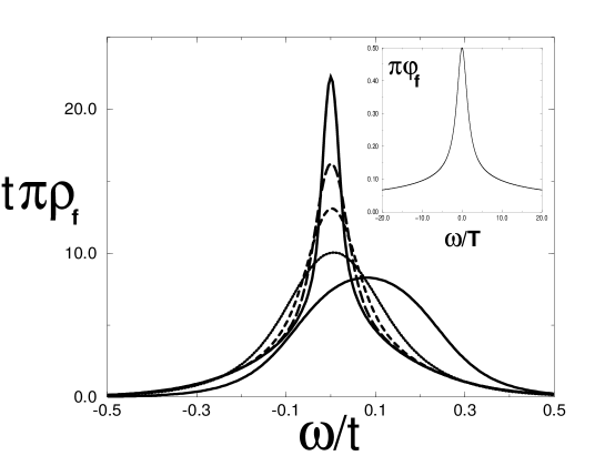
FIG. 7.: Spectral functions $\pi\rho_{f}(\omega)$ for $\delta=0.04$ and $J/t=0.3$ (corresponding to $\epsilon_{F}^{*}/J\simeq 1.8\,10^{-2}$). The different curves correspond from top to bottom to $T/t=1/200,1/50,1/25,1/10,1$. Inset : thermal scaling function Eq. (60)

FIG. 8.: Local dynamical susceptibility $\chi_{\mbox{loc}}^{\prime\prime}(\omega)$ for $\delta=0.04$ and $J/t=0.3$. The different curves correspond from top to bottom to $T/t=1/200,1/50,1/25,1/10,1/5,1$. In the temperature range $\epsilon_{F}^{*}<T<J$ and for frequencies $\omega<J$, these curves scale on the universal form $\chi_{loc}^{\prime\prime}(\omega,T)=\frac{\sqrt{\pi}}{2J}\tanh\frac{\omega}{2T}$

FIG. 9.: Scaling function $\psi$ associated with the NMR relaxation rate : $J/T_{1}=\psi(T/\epsilon_{F}^{*})$

FIG. 10.: Scaling function for the resistivity. Inset : low temperature Fermi liquid regime

FIG. 11.: Real part of the optical conductivity $\mathop{\hbox{Re}}\sigma(\omega)$ versus $\omega$, for $\delta=0.04$ and $J/t=0.3$. The different curves correspond to $T/t=1/200,1/100,1/50,1/25,1/10$. Here $\epsilon_{F}^{*}/t=1.8\,10^{-2}$. Inset : the curve corresponding to $T/t=1/100$, plotted in log-log coordinates, in the frequency range $T\sim\epsilon_{F}^{*}<\omega<J$. The $1/\omega$ behaviour described in the text is clearly visible.

FIG. 12.: Schematic crossover diagram for cuprates illustrating : i) the existence of a metal-insulator transition as a function of doping at $T=0$ and ii) the possible relevance of our model to the corresponding quantum critical regime (other features like the pseudogap and the Néel temperature have not been depicted)

FIG. 13.: $1/\chi(T)$ (solid line) and $1/\chi_{\mbox{loc}}(T)\sim 1/\ln T$ (dashed line) versus $T$ as calculated numerically in the undoped model.

REFERENCES

- [1] W.F. Brinkman and T.M. Rice, Phys. Rev. B 2, 4302 (1970).
- [2] For reviews on the large- approach, see e.g D.M. Newns and N. Read, Adv. Phys. 36, 799 (1987) and G. Kotliar, in “Strongly Interacting Fermions and High Superconductivity”, B.Doucot and J. Zinn-Justin eds., (Elsevier Science Pub.) (1994).
- [3] For a review, see A.Georges, G.Kotliar, W.Krauth and M.Rozenberg, Rev. Mod. Phys. 68, 13 (1996).
- [4] F.C. Chou, N.R. Belk, M.A. Kastner, R.J. Birgeneau and A. Aharony Phys. Rev. Lett. 75, 2204 (1995).
- [5] Y. Ando, G.S. Boebinger, A. Passner, T. Kimura and K. Kishio Phys. Rev. Lett. 75, 4662 (1995).
- [6] G.S. Boebinger, Y. Ando, A. Passner, T. Kimura, M. Okuya, J. Shimoyama, K. Kishio, K. Tamasaku, N. Ichikawa and S. Uchida Phys. Rev. Lett. 77, 5417 (1996).
- [7] A. Aharony, R.J. Birgeneau, A. Coniglio, M.A. Kastner and H.E. Stanley Phys. Rev. Lett. 60, 1330 (1988).
- [8] S.M. Hayden, G. Aeppli, H. Mook, D. Rytz, M.F. Hundley and Z. Fisk Phys. Rev. Lett. 66, 821 (1991).
- [9] S.M. Hayden, G. Aeppli, H. Mook, T.G. Perring, T.E. Mason, S.-W. Cheong and Z. Fisket al., Phys. Rev. Lett. 76, 1344 (1996).
- [10] B. Keimer, N. Belk, R.J. Birgeneau, A. Cassanho, C.Y. Chen, M. Greven, M.A. Kastner, A. Aharony, Y. Endoh, R.W. Erwin and G. Shirane Phys. Rev. B 46, 14034 (1992).
- [11] S. Petit, PhD Thesis, Université Paris-Sud, unpublished, (1997).
- [12] G. Aeppli, T.E. Mason, S.M. Hayden, H.A. Mook and J. Kulda Science 278, 1432 (1997).
- [13] For a review of neutron experiments on LSCO at low doping, see M.A. Kastner, R.J. Birgenau, G. Shirane and Y. Endoh, preprint, to appear in Rev. Mod. Phys.
- [14] For a review of neutron experiments on YBCO, see P. Bourges, to appear in The gap symmetry and fluctuations in high-temperature superconductors, Proceedings of the NATO Cargese summer school, J. Bok, G. Deutscher, D. Pavuna and S.A. Wolf Eds (Plenum, 1998).
- [15] Y. Sidis, PhD Thesis, Université Paris-Sud, unpublished, (1995).
- [16] P. Mendels, H. Alloul, J.H. Brewer, G.D. Morris, T.L. Duty, S. Johnston, E.J. Ansaldo, G. Collin, J.F. Marucco, C. Niedermayer, D.R. Noakes and C.E. Stronach Phys. Rev. B. Rapid. Comm. 49 10035 (1994)
- [17] S. Sachdev and J. Ye Phys. Rev. Lett. 70, 3339 (1993).
- [18] This is true for fermionic representations and for bosonic representations with small enough “size” of the spin.
- [19] C.M. Varma, P. Littlewood, S. Schmitt-Rink, E. Abrahams and A. Ruckenstein, Phys. Rev. Lett. 63, 1996 (1989).
- [20] A. Virosztek and J. Ruvalds, Phys. Rev. B 42, 4064 (1990).
- [21] We note that the two-dimensional quantum XY model with bond disorder has been suggested to have a spin-liquid ground state for a large enough concentration of frustrating bonds: see P.Gawiec and D. Grempel, Phys. Rev. B 54, 3343 (1996).
- [22] S. Doniach Physica B 91 231 (1977)
- [23] See e.g. : F. Steglich, B. Buschinger, P. Gegenwart, M. Lohmann, R. Helfrich, C. Langhammer, P. Hellmann, L. Donnevert, S. Thomas, A. Link, C. Geibel, M. Lang, G. Sparn and W. Assmus J. Phys.:Condens Matter 8 9909 (1996); M.B. Maple, M.C. de Andrade, J. Herrmann, Y. Dalichaouch, D.A. Gajewski, C.L. Seaman, R. Chau, R. Movshovich, M.C. Aronson and R. Osborn J. Low Temp. Phys. 99 223 (1995)
- [24] M. Horbach and A. Ruckenstein, private communication
- [25] For reviews, see e.g D.M. Newns and N. Read, Adv. Phys. 36, 799 (1987) and G. Kotliar, in “Strongly Interacting Fermions and High Superconductivity”, B.Doucot and J. Zinn-Justin eds., (Elsevier Science Pub.) (1994).
- [26] We note that our conventions for Green’s functions are different than those in Ref.[17].
- [27] Only part of the degeneracy is actually removed: the spin-liquid ground-state turns out to have an extensive entropy in the large- limit, as studied in detail in [29]. b
- [28] A. M. Sengupta Preprint cond-mat 9707316; A. Georges and A.M. Sengupta, unpublished.
- [29] A. Georges, O. Parcollet and S. Sachdev in preparation.
- [30] O. Parcollet and A. Georges, Phys. Rev. Lett. 79 4665 (1997); O. Parcollet, A. Georges, G. Kotliar and A. Sengupta, to appear in Phys. Rev. B.
- [31] Note that strictly speaking there is no Fourier transform on the Bethe lattice. k-dependence should really be interpreted as a dependence on the single-particle tight binding energy .
- [32] A. Abrikosov, L. P. Gorkov and I. E. Dzialoshinski, Methods of Quantum Field Theory in Statistical Physics, Pergamon, Elmsford N.Y (1965).
- [33] See e.g. chapter 24 in A. M. Tsvelik “Quantum Field Theory in Condensed Matter Physics”, Cambridge University Press, 1995.
- [34] I.S. Gradshteyn and I.M. Ryzhik Table of integrals, series and products, Academic Press, 1980
- [35] A. Chubukov, Phys. Rev. B 52, R3840 (1995) and preprint cond-mat 9709221; A.Millis, Phys. Rev. B 45, 13047 (1995); A.V Chubukov and J. Schmalian, Phys. Rev. B, to appear.
- [36] S. Misra, R. Gatt, T. Schmauder, A.V. Chubukov, M. Onellion, M. Zacchigna, I. Vobornik, F. Zwick, M. Grioni, G. Margaritondo, C. Quitmann and C. Kendziora preprint cond-mat 9805297
- [37] N. Furukawa and M. Imada J. Phys. Soc. Jpn 61 3331 (1992); ibid. 62 2557 (1993); M. Imada J. Phys. Soc. Jpn 64 2954 (1995); F. F. Assaad and M. Imada Phys. Rev. Lett 76 3176 (1996).
- [38] D. R. Grempel and M. J. Rozenberg, Phys. Rev. Lett. 80 389 (1998)
- [39] H. Takagi, B. Batlogg, H.L. Kao, J. Kwo, R.J. Cava, J.J. Krajewski and W.F. Peck, Jr. Phys. Rev. Lett. 69, 2975 (1992)
- [40] E. Abrahams, J. Phys I France 6 2191 (1996).
- [41] A. El Azrak, R. Nahoum, N. Bontemps, M. Guilloux-Viry, C. Thivet, A. Perrin, S. Labdi, Z.Z. Li and H. Raffy Phys. Rev. B 49, 9846 (1994).
- [42] C. Baraduc, A. El Azrak and N. Bontemps, Journal of Superconductivity 9, 3 (1996).
- [43] N. M. Salem and R. J. Gooding, cond-mat 9607154; R.J. Gooding, N. M. Salem, R.J Birgenau and F.C. Chou, cond-mat 9611166.
- [44] S.R. White and D.J. Scalapino Preprints cond-mat 9705128 and 9801274.
- [45] A.I. Lichtenstein, M. Fleck, A.M. Oleś and L. Hedin, unpublished ; M. Fleck private communication
- [46] S.Petit, private communication and [11]; G. Aeppli, personal communication.
- [47] J.R. Cooper and J.W. Loram, J. Phys. I France 6 2237 (1996)