High Temperature Conductance of the Single Electron Transistor

Abstract

The linear conductance of the single electron transistor is determined in the high temperature limit. Electron tunneling is treated nonperturbatively by means of a path integral formulation and the conductance is obtained from Kubo’s formula. The theoretical predictions are valid for arbitrary conductance and found to explain recent experimental data.

Considering applications of single electron tunneling, one is faced with a dilemma. On the one hand, the conventional approach [1] consider systems with small tunneling conductance $G_{T}\ll G_{K}=e^{2}/h$ implying nearly perfect charge quantization. On the other hand, when using these devices, e.g. as highly sensitive electrometers [2] or for thermometry [3], a large current signal is desirable meaning large tunneling conductance. Since for $G_{T}\gg G_{K}$ charging effects disappear, a compromise must be found in practice. This problem has spurred considerable interest in the precise behavior of single charge tunneling devices for large conductance [4, 5].

FIG. 1.: Circuit diagram of the single electron transistor.

In this letter, we consider the single electron transistor (SET) at high temperatures for arbitrary tunneling conductance of the junctions. The SET consists of two tunnel junctions in series, with tunneling conductance $G_{1}$ and $G_{2}$ and capacitance $C_{1}$ and $C_{2}$, respectively, biased by a voltage source $V$ which may be split among the left and right branches into $\rho_{1}V$ and $\rho_{2}V$ with $\rho_{1}+\rho_{2}=1$, cf. Fig. 1. The island in between the junctions is connected via a gate capacitance $C_{g}$ to a control voltage $U_{g}$ shifting the electrostatic energy of the system continuously. The important energy scale is the charging energy $E_{c}=e^{2}/2C$ with the island capacitance $C=C_{1}+C_{2}+C_{g}$. For weak electron tunneling, $E_{c}$ is the energy needed to charge the island with one excess electron at vanishing gate voltage $U_{g}=0$. Due to the periodicity of the Hamiltonian in $U_{g}$, the conductance is a periodic function with period 1 of the dimensionless voltage $n_{g}=U_{g}C_{g}/e$ [6]. Specifically, we are interested in the linear dc conductance for small transport voltage, that may be calculated from the Kubo formula

$$\!G=\lim_{\omega\rightarrow 0}\frac{1}{\hbar\omega}{\rm Im}\lim_{i\nu_{l}\rightarrow\omega+i\delta}\int_{0}^{\hbar\beta}\!\!\!d\tau e^{i\nu_{l}\tau}\langle I^{(1)}(\tau)I^{(2)}(0)\rangle.$$ (1)

Since the dc current through both junctions coincides, the first current operator $I^{(1)}$ may be an arbitrary linear combination $I^{(1)}=\epsilon_{1}I_{1}-\epsilon_{2}I_{2}$ (with $\epsilon_{1}+\epsilon_{2}=1$) of the current operators $I_{1}$ and $I_{2}$ through junctions $1$ and $2$, respectively. The relative ”$-$” sign comes from the opposite directions of $I_{1}$ and $I_{2}$, which are both positive for flux onto the island. The second current operator $I^{(2)}=\kappa_{1}I_{1}-\kappa_{2}I_{2}$, with the relative weights $\kappa_{1}=(C_{2}+\rho_{1}C_{g})/C$ and $\kappa_{2}=(C_{1}+\rho_{2}C_{g})/C$, is determined by linear response theory from the coupling of the transport voltage $V$. To evaluate the current-current correlator we employ a generating functional

$$\!Z[\xi_{1},\xi_{2}]={\rm tr}\,T_{\tau}\exp\!\!\left\{\!-\frac{1}{\hbar}\int_{0}^{\hbar\beta}\!\!\!d\tau\bigg{[}H-\!\sum_{i=1,2}\!I_{i}\xi_{i}(\tau)\bigg{]}\!\right\},$$ (2)

where $H$ is the Hamiltonian of the system for $V=0$, and $T_{\tau}$ is the time ordering operator for imaginary times $\tau$. The correlator is then given by a second order variational derivative relative to the auxiliary fields $\xi_{1}$ and $\xi_{2}$. In the phase representation [7], we get for the generating functional

$$Z[\xi_{1},\xi_{2}]=\int D[\varphi]\exp\left\{-\frac{1}{\hbar}S[\varphi,\xi_{1},\xi_{2}]\right\},$$ (3)

with the effective action

$$S[\varphi,\xi_{1},\xi_{2}]=S_{c}[\varphi]+S_{1}[\varphi,\xi_{1}]+S_{2}[\varphi,\xi_{2}].$$ (4)

The first term on the rhs is the Coulomb action

$$S_{c}[\varphi]=\int_{0}^{\hbar\beta}d\tau\left[\frac{{\dot{\varphi}}^{2}(\tau)}{4E_{c}}-in_{\rm g}{\dot{\varphi}}(\tau)\right]$$ (5)

describing the Coulomb charging of the island in presence of an applied gate voltage, and the effective tunneling actions $(i=1,2)$

$$S_{i}[\varphi,\xi_{i}] = g_{i}\int_{0}^{\hbar\beta}d\tau d\tau^{\prime}\alpha(\tau-\tau^{\prime})$$ (7)

$$(1-ie\xi_{i}(\tau))(1+ie\xi_{i}(\tau^{\prime}))e^{i[\varphi(\tau)-\varphi(\tau^{\prime})]}$$

describe quasi-particle tunneling through junctions $1$ and $2$, respectively. Here $g_{i}=G_{i}/G_{K}$ is the dimensionless conductance of junction $i$, and the kernel $\alpha(\tau)$ may be written as Fourier series

$$\alpha(\tau)=-\frac{1}{4\pi\beta}\sum_{n=-\infty}^{\infty}|\nu_{n}|\,e^{-i\nu_{n}\tau},$$ (8)

where the $\nu_{n}=2\pi n/\hbar\beta$ are Matsubara frequencies. For vanishing auxiliary fields the action reduces to the action of the single electron box [5] and thus the generating functional reduces to the box partition function $Z=Z[0,0]$. Performing the variational derivatives explicitly, we get for the correlator

$$\langle I_{j}(\tau)I_{j^{\prime}}(\tau^{\prime})\rangle=\langle I_{j}(\tau)I_{j}(\tau^{\prime})\rangle^{E}\delta_{j,j^{\prime}}+\langle I_{j}(\tau)I_{j^{\prime}}(\tau^{\prime})\rangle^{F}.$$ (9)

Since the auxiliary fields are in the argument of an exponential, there are two contributions. The first term comes from the second order variational derivative of the action and reads

$$\langle I_{j}(\tau)I_{j}(\tau^{\prime})\rangle^{E} = \frac{2e^{2}}{\hbar}g_{j}\alpha(\tau-\tau^{\prime})\frac{1}{Z}\int D[\varphi]$$ (11)

$$\exp\left\{-\frac{1}{\hbar}S[\varphi]\right\}\cos[\varphi(\tau)-\varphi(\tau^{\prime})],$$

with the box action $S[\varphi]=S[\varphi,\xi_{1}=0,\xi_{2}=0]$. The second term in Eq. $(\ref{eq:corr0})$ involves a multiplication of two current functionals arising as first order variational derivatives of the action

$$\langle I_{j}(\tau)I_{j^{\prime}}(\tau^{\prime})\rangle^{F} = g_{j}g_{j^{\prime}}\frac{1}{Z}\int D[\varphi]$$ (13)

$$\exp\left\{-\frac{1}{\hbar}S[\varphi]\right\}I[\varphi,\tau]I[\varphi,\tau^{\prime}],$$

with the current functional

$$I[\varphi,\tau]=\frac{2e}{\hbar}\int_{0}^{\hbar\beta}d\tau^{\prime}\alpha(\tau-\tau^{\prime})\sin[\varphi(\tau)-\varphi(\tau^{\prime})].$$ (14)

Taking into account that $\langle I_{j}(\tau)I_{j}(\tau^{\prime})\rangle^{E}/g_{j}$ and $\langle I_{j}(\tau)I_{j^{\prime}}(\tau^{\prime})\rangle^{F}/g_{j}g_{j^{\prime}}$ depend only on the dimensionless parallel conductance $g=g_{1}+g_{2}$ and thus are independent of the indices $j$ and $j^{\prime}$, the conductance may be written as

$$G = \epsilon_{1}\kappa_{1}(g_{1}E+g_{1}^{2}F)-2\epsilon_{1}\kappa_{2}g_{1}g_{2}F$$ (16)

$$+\epsilon_{2}\kappa_{2}(g_{2}E+g_{2}^{2}F),$$

where

$$\!E=\lim_{\omega\rightarrow 0}\frac{1}{\hbar\omega}{\rm Im}\lim_{i\nu_{l}\rightarrow\omega+i\delta}\int_{0}^{\hbar\beta}\!d\tau\,e^{i\nu_{l}\tau}\frac{\langle I_{1}(\tau)I_{1}(0)\rangle^{E}}{g_{1}}$$ (17)

and

$$\!F=\lim_{\omega\rightarrow 0}\frac{1}{\hbar\omega}{\rm Im}\lim_{i\nu_{l}\rightarrow\omega+i\delta}\int_{0}^{\hbar\beta}\!d\tau\,e^{i\nu_{l}\tau}\frac{\langle I_{1}(\tau)I_{1}(0)\rangle^{F}}{g_{1}^{2}}$$ (18)

Since the conductance does not depend on the specific choice of the parameters $\epsilon_{i}$ and $\rho_{i}$, we then find that

$$G=E/(G_{1}^{-1}+G_{2}^{-1}),$$ (19)

This is a formally exact expression for the linear dc conductance.

To proceed, we make explicit the sum over winding numbers $k$ of the phase and write the correlator (11) in the form

$$\langle I_{1}(\tau)I_{1}(0)\rangle^{E}/g_{1} = \frac{2e^{2}}{\hbar}\alpha(\tau)\frac{1}{Z}\sum_{k=-\infty}^{\infty}\int\limits_{\varphi(0)=0}^{\varphi(\hbar\beta)=2\pi k}D[\varphi]$$ (21)

$$\exp\left\{-\frac{1}{\hbar}S[\varphi]\right\}\cos[\varphi(\tau)-\varphi(0)].$$

For given winding number $k$, the path integral may be evaluated approximately by expanding about the classical path ${\bar{\varphi}}(\tau)=\varphi(0)+\nu_{k}\tau$. An arbitrary path of winding number $k$ is of the form $\varphi(\tau)={\bar{\varphi}}(\tau)+\zeta(\tau)$ with $\zeta(0)=\zeta(\hbar\beta)=0$, and the action can be written in terms of the Fourier coefficients $\zeta_{n}=\zeta_{n}^{\prime}+i\zeta_{n}^{\prime\prime}$ as

$$\!\!\!S[{\bar{\varphi}}+\zeta]=-2\pi ikn_{g}+S_{\rm cl}^{(k)}+\delta^{2}S^{(k)}+\delta^{4}S^{(k)}+...\,.$$ (22)

Here

$$S_{\rm cl}^{(k)}=\frac{\pi^{2}k^{2}}{\beta E_{c}}+|k|\frac{g}{2},$$ (23)

is the action of the classical path. The second term reads

$$\delta^{2}S^{(k)}=\sum_{n=1}^{\infty}\lambda_{n}^{(k)}\left(\zeta_{n}^{\prime 2}+\zeta_{n}^{\prime\prime 2}\right),$$ (24)

with the eigenvalues

$$\lambda_{n}^{(k)}=\frac{2\pi^{2}n^{2}}{\beta E_{c}}+g\Theta(n-|k|)(n-|k|).$$ (25)

The term $\delta^{4}S^{(k)}$ is of fourth order in the Fourier components $\zeta_{n}$ and not given explicitly here. Since the $\lambda_{n}^{(k)}$ are large for small $\beta E_{c}$, the expansion $(\ref{eq:action})$ about the classical path converges rapidly for high temperatures.

Rewriting the cosine function in Eq. $(\ref{eq:korr1})$ as a sum of exponentials, we get for the correlator the expansion

$$\langle I_{1}(\tau)I_{1}(0)\rangle^{E}/g_{1}=\frac{2e^{2}}{\hbar}\alpha(\tau)\frac{1}{Z}\sum_{k=-\infty}^{\infty}C_{k}e^{2\pi ikn_{g}}\cos(\nu_{k}\tau)\exp\left[-2\sum_{n=1}^{\infty}\frac{1-\cos(\nu_{n}\tau)}{\lambda_{n}^{(k)}}\right]\left[1+S_{4}^{(k)}+...\right],$$ (26)

where the coefficients $C_{k}$ read

$$C_{k}=\frac{\Gamma(1+k_{+})\Gamma(1+k_{-})}{\Gamma^{2}(1+k)\Gamma(1+u)}e^{-S_{\rm cl}^{(k)}},$$ (27)

with $k_{\pm}=k+\frac{u}{2}\pm\frac{1}{2}\sqrt{4uk+u^{2}}$ and $u=g\beta E_{c}/2\pi^{2}$. The dominant corrections to the semiclassical approximation are described by

$$S_{4}^{(k)} = -\frac{1}{2}g\hbar\beta\sum\limits_{m,n\not=0}\frac{1}{\lambda_{m}^{(k)}\lambda_{n}^{(k)}}\Big{[}{\tilde{\alpha}}(\nu_{k})-2{\tilde{\alpha}}(\nu_{n+k})$$ (29)

$$\quad-2{\tilde{\alpha}}(\nu_{n-k})+{\tilde{\alpha}}(\nu_{m+n+k})+{\tilde{\alpha}}(\nu_{m+n-k})\Big{]}.$$

The corresponding expansion of the partition function $Z$ reads

$$Z=\sum_{k=-\infty}^{\infty}C_{k}e^{2\pi ikn_{g}}\left[1+S_{4}^{(k)}+...\right],$$ (30)

with the same correction $(\ref{eq:fourth})$. The expansions $(\ref{eq:korr2})$ and $(\ref{eq:partition})$ proceed in powers of $\beta E_{c}$, however, terms involving $u=g\beta E_{c}/2\pi^{2}$ are kept to all orders. This ensures a meaningful result in the limit of moderately high temperatures also for large conductance $g$.

From Eq. $(\ref{eq:korr2})$ one obtains for the Fourier coefficients

$$E(\nu_{l})=\int_{0}^{\hbar\beta}d\tau\,e^{i\nu_{l}\tau}\langle I_{1}(\tau)I_{1}(0)\rangle^{E}/g_{1}$$ (31)

the high temperature expansion

$$\!E(\nu_{l})\!=\!\frac{4\pi}{\hbar}\frac{1}{Z}\!\sum\limits_{k=-\infty}^{\infty}\!\!C_{k}e^{2\pi ikn_{g}}\exp\left[\!-2\sum\limits_{n=1}^{\infty}\frac{1}{\lambda_{n}^{(k)}}\right]\!\left\{{\tilde{\alpha}}(\nu_{l+k})+\!\sum\limits_{m\not=0}\!\!\frac{{\tilde{\alpha}}(\nu_{l+k+m})}{\lambda_{m}^{(k)}}+\!\frac{1}{2}\!\sum\limits_{m,n\not=0}\!\!\frac{{\tilde{\alpha}}(\nu_{l+k+m+n})}{\lambda_{m}^{(k)}\lambda_{n}^{(k)}}+{\tilde{\alpha}}(\nu_{l+k})S_{4}^{(k)}\!+\!...\right\}\!.$$ (32)

When these coefficients are analytically continued in the complex $\nu$ plane, they are analytic on each half plane Re$\,\nu{{\lower 2.0pt\hbox{$<$}\atop\raise 5.0pt\hbox{$>$}}}0$ with a cut along the imaginary axis [8]. The representation of $E(\nu)$ as a sum over winding numbers $k$ shifts this cut to Re$\,\nu=k$ for the $k\,$th term of the sum. Thus, in the phase representation, only the full sum shows the analytic properties underlying the conductance formula $(\ref{eq:kubo1})$. To deal with this problem we formally change to the charge representation, perform the analytic continuation and the $\omega\rightarrow 0$ limit there, and then go back to the phase representation. This way the high temperature expansion of the conductance $(\ref{eq:kubo2})$ may be evaluated to read

$$G = [1/(G_{1}^{-1}+G_{2}^{-1})]Z^{-1}\exp\left\{-2[\gamma+\psi(1+u)]/g\right\}$$ (35)

$$\big{\{}1-\psi^{\prime}(1+u)(\beta E_{c}/\pi^{2})$$

$$\hskip 14.22636pt+\left[g\sigma(u)+\tau(u)\right](\beta E_{c}/2\pi^{2})^{2}+{\cal O}(\beta E_{c})^{3}\big{\}}.$$

The dependence on $u=g\beta E_{c}/2\pi^{2}$ is given in terms of the digamma function $\psi(z)$ and two auxiliary functions

$$\sigma(u) = \frac{\gamma+\psi(1+u)-u\psi^{\prime}(1+u)}{u^{2}}$$ (37)

$$+\int_{0}^{1}\!\mbox{d}v\,\frac{2v(1-v^{u})\phi(v,1,1+u)}{(1-v)u}$$

and

$$\tau(u) = \frac{\pi^{2}}{6u}\psi(1+u)-\frac{[\psi(1+u)+\gamma]^{2}}{u^{2}}+\int_{0}^{1}\!\mbox{d}v\,\Xi(u,v)$$ (39)

$$-\frac{3\gamma\psi^{\prime}(1+u)+\psi(1+u)[\frac{\pi^{2}}{6}+2\psi^{\prime}(1+u)]}{u},$$

with Lerch’s transcendent $\phi(z,u,v)$ [9] and

$$\Xi(u,v) = \frac{\psi^{\prime}(1+u)}{u\ln(v)}+\frac{1}{(1-v)u}\Bigg{\{}\frac{1-2v^{u}}{v}\left[\ln(v)\phi(\frac{1}{v},1,1+u)+\phi(\frac{1}{v},2,1+u)\right]+2v\phi(v,2,1+u)$$ (41)

$$-\frac{2(1-v^{u})}{u}\left[\ln(1-v)+v\phi(v,1,1+u)\right]+v^{u}\left[2\ln(v)\ln(1-v)+{1\over 2}\ln^{2}(v)+3\mbox{Li}_{2}(1-v)\right]\Bigg{\}}.$$

The high temperature expansion of $Z$ is straightforward and reads

$$Z = 1+g\sigma(u)(\beta E_{c}/2\pi^{2})^{2}+{\cal O}(\beta E_{c})^{3}$$ (43)

$$\hskip 8.5359pt+2C_{1}\cos(2\pi n_{g})\left[1+{\cal O}(\beta E_{c})^{2}\right],$$

which combines with Eq. $(\ref{conductance})$ to yield an analytical expression for the high temperature conduction of a SET valid for arbitrary tunneling conductance.

In the region of weak tunneling, $g<1$, the quantity $u$ becomes small at high temperatures and we may replace $\sigma(u)$ and $\tau(u)$ by

$$\sigma(0)=3\zeta(3),\qquad\tau(0)=\pi^{4}/10.$$ (44)

This gives for the conductance of a weakly conducting SET

$$\!\!G = \frac{1}{G_{1}^{-1}+G_{2}^{-1}}\bigg{\{}1-\frac{\beta E_{c}}{3}$$ (46)

$$\qquad\quad+\left[\frac{1}{15}+g\frac{3\zeta(3)}{2\pi^{4}}\right](\beta E_{c})^{2}+{\cal O}(\beta E_{c})^{3}\bigg{\}},$$

in accordance with earlier work [10]. In the region of strong tunneling the quantity $u$ is typically large even for the highest temperatures explored experimentally and the full expression $(\ref{conductance})$, $(\ref{partition})$ must be used.

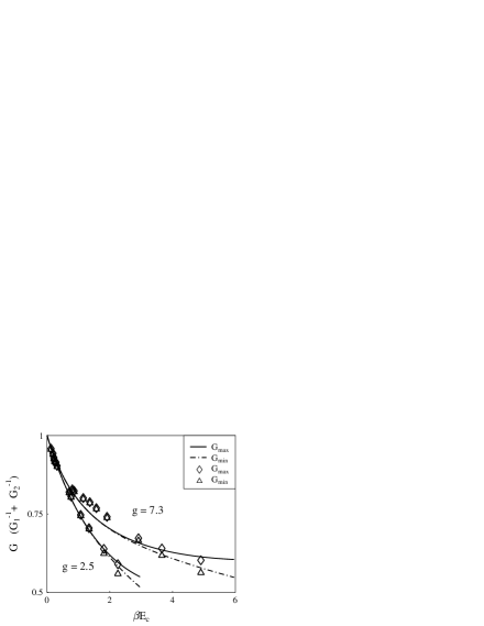
FIG. 2.: Maximum and minimum linear conductance in dependence on dimensionless temperature for two dimensionless parallel conductances $\alpha=2.5$ and $7.3$ compared with experimental data (symbols) by Joyez et al. [11].

We have compared our findings with recent experimental data by Joyez et al. [11] for transistors with $g=0.6$, $2.5$ and $7.3$. As seen from Fig. 2 the theory describes the high temperature behavior of all junctions (results for $g=0.6$ are not shown) down to temperatures where the current starts to modulate with the gate voltage. The parameters have not been adjusted to improve the fit but coincide with the values given in [11]. The small deviations between theory and experiment for $g=7.3$ near $\beta E_{c}=1$ may arise from experimental uncertainties in $\beta E_{c}$. We mention that the temperature dependence of the conductance of the highly conducting SET ($g=7.3$) is not within reach of previous theoretical predictions. The results obtained thus present substantial progress and should be useful for experimental studies of even larger tunneling conductances since the predictions remain valid for arbitrary values of $g$.

The authors would like to thank Michel Devoret, Daniel Esteve, and Philippe Joyez for valuable discussions. Financial support was provided by the Deutsche Forschungsgemeinschaft (DFG) and the Deutscher Akademischer Austauschdienst (DAAD).

REFERENCES

• [1] Single Charge Tunneling, H. Grabert, M.H. Devoret (eds.), NATO ASI Series B, Vol. 294 (Plenum, NY, 1992).
• [2] T.A. Fulton and G.J. Dolan, Phys. Rev. Lett. 59, 109 (1987).
• [3] J.P. Pekola, K.P. Hirvi, J.P. Kauppinen, and M.A. Paalanen, Phys. Rev. Lett. 73, 2903 (1994).
• [4] H. Grabert, Phys. Rev. B 50, 17364 (1994); H. Schoeller and G. Schön, Phys. Rev. B 50, 18436 (1994); G. Göppert, X. Wang, and H. Grabert, Phys. Rev. B 55, R10213 (1997); D.S. Golubev, J. König, H. Schoeller, G. Schön, and A.D. Zaikin, Phys. Rev. B 56, 15782 (1997).
• [5] X. Wang and H. Grabert, Phys. Rev. B 53, 12621 (1996).
• [6] D.V. Averin and K.K. Likharev, in Mesoscopic Phenomena in Solids, ed. by B.L. Altshuler, P.A. Lee, and R.A. Webb, p. 173 (North-Holland, Amsterdam, 1991).
• [7] G. Schön and A.D. Zaikin, Phys. Rep. 198, (1990).
• [8] G. Baym and N.D. Mermin, J. Math. Phys. 2, 232 (1961).
• [9] W. Magnus, F. Oberhettinger, and R.P. Soni, Formulas and Theorems for the Special Functions of Mathematical Physics (Springer, Berlin, 1966)
• [10] G. Göppert, Diploma thesis, Freiburg 1996; P. Joyez and D. Esteve, Phys. Rev. B 56, 1848 (1997).
• [11] P. Joyez, V. Bouchiat, D. Esteve, C. Urbina, and M.H. Devoret, Phys. Rev. Lett. 79, 1349 (1997).