Active Walker Model for the Formation of Human and Animal Trail Systems
Abstract
Active walker models have recently proved their great value for describing the formation of clusters, periodic patterns, and spiral waves as well as the development of rivers, dielectric breakdown patterns, and many other structures. It is shown that they also allow to simulate the formation of trail systems by pedestrians and ants, yielding a better understanding of human and animal behavior. A comparison with empirical material shows a good agreement between model and reality.
Our trail formation model includes an equation of motion, an equation for environmental changes, and an orientation relation. It contains some model functions, which are specified according to the characteristics of the considered animals or pedestrians. Not only the kind of environmental changes differs: Whereas pedestrians leave footprints on the ground, ants produce chemical markings for their orientation. Nevertheless, it is more important that pedestrians steer towards a certain destination, while ants usually find their food sources by chance, i.e. they reach their destination in a stochastic way. As a consequence, the typical structure of the evolving trail systems depends on the respective species. Some ant species produce a dendritic trail system, whereas pedestrians generate a minimal detour system.
The trail formation model can be used as a tool for the optimization of pedestrian facilities: It allows urban planners to design convenient way systems which actually meet the route choice habits of pedestrians.
pacs:
05.40.+j,61.43.-j,82.30.Nr,89.50.+rI Introduction
The emergence of complex behavior in a system consisting of simple, interacting elements [1, 2, 3] is among the most fascinating phenomena of our world. Examples can be found in almost every field of today’s scientific interest, ranging from coherent pattern formation in physical and chemical systems [4, 5, 6], to the motion of animal swarms in biology [7, 8], and the behavior of social groups [9, 10, 11].
In the life and social sciences, one is usually convinced that the evolution of social systems is determined by numerous factors, such as cultural, sociological, economic, political, ecological etc. However, in recent years, the development of the interdisciplinary field “science of complexity” has lead to the insight that complex dynamic processes may also result from simple interactions, and even social structure formation could be well described within a mathematical approach [10, 11, 12, 13, 14]. Moreover, at a certain level of abstraction, one can find many common features between complex structures in very different fields.
A recent field of particular interest is the microsimulation of self-organization phenomena occuring in traffic systems. This includes the formation of jammed states in freeway or city traffic [15, 16, 17, 18, 19, 20, 21, 22, 23, 24, 25, 26, 27, 28] as well as the various collective patterns of motion developing in pedestrian crowds [28, 29, 30, 31, 32] like oscillatory changes of the walking direction at narrow passages or round-about traffic at crossings.
In this paper, we draw the attention to the specific collective phenomenon of trail formation [33, 34], which is widely spread in the world of animals and humans. Regarding their shape, duration and extension, trail systems of different animal species and humans differ, of course. However, more striking is the question, whether there is a common underlying dynamics which allows for a generalized description of the formation and evolution of trail systems.
As our experience tells us, trails are adapted to the requirements of their users. In the course of time, frequently used trails become more developed, making them more attractive, whereas rarely used trails vanish again. Trails with large detours become optimized by creating shortcuts. New destinations or entry points are connected to an existing trail system. These dynamical processes occur basically without any common planning or direct communication among the users. Instead, the adaptation process can be understood as a self-organization phenomenon, resulting from the non-linear feedback between the users and the trails [35].
In order to simulate this process, we propose here a particle-based, multi-agent approach to structure formation, which belongs to the class of active walker models. Like random walkers, active walkers are subject to fluctuations and influences of their environment. However, they are additionally able to locally change their environment, e.g. by altering an environmental potential, which in turn influences their further movement and their behavior. In particular, changes produced by some walkers can influence other walkers. Hence, the non-linear feedback can be interpreted as an indirect interaction between the active walkers via environmental changes, which may lead to the self-organization of spatial structures.
Active walker models have proved their versatility in a variety of applications, such as formation of complex structures [36, 37, 38, 39, 40, 41, 42], pattern formation in physico-chemical systems [43, 44, 45, 46], aggregation in biological [47, 48] or urban [49] systems, and generation of directed motion [50, 51]. The approach provides a quite stable and fast numerical algorithm for simulating processes involving large density gradients, and it is applicable also in cases where only small particle numbers govern the structure formation. In particular, the active walker model is applicable to processes of pattern formation which are intrinsically determined by the history of their creation, such as the formation of trail systems, discussed in this paper.
In Section II, the active walker model for trail formation is formulated in terms of a Langevin equation for the movement of the walkers, an equation for environmental changes, and a relation describing the orientation of the walkers with respect to existing trails. As one application of the model, Section III describes the formation of trunk trails in ant colonies, which are commonly used to exploit food sources. As a second application, in Section IV the evolution of pedestrian trail systems is modelled. Both Sections III and IV present a comparison of computational results with real trail systems, indicating a good aggrement between model and empirical facts. In Section IV.A, the equations for pedestrian trail systems are scaled to dimensionless equations, in order to demonstrate that the evolving trail systems are (apart from the boundary conditions) only determined by two parameters. In Section IV.B, a macroscopic formulation of human trail formation is derived from the microscopic equations, allowing analytical investigations and an efficient calculation of the stationary solution by a self-consistent field method. Our conclusions and an outlook, which suggests an application of the model to the optimization of trail systems, are presented in Section V.
II Active walker model of trail formation
In order to introduce our model, we first describe the process of trail formation within a general stochastic framework. Hence, in this section the active walkers are not specified as pedestrians or animals. Rather, they are considered as arbitrary moving agents, who continuously change their environment by leaving markings while moving. These markings can, for example, be imagined as damaged vegetation on the ground (as in the case of hoofed animals or pedestrians) or as chemical markings (as in the case of ants).
The spatio-temporal distribution of the existing markings will be described by a ground potential . Trails are characterized by particularly large values of . The subscript allows to distinguish different kinds of markings. Due to weathering or chemical decay, the markings have a certain life time which characterizes their local durability. Therefore, existing trails tend to fade, and the ground potential would exponentially adapt to the natural ground conditions , if the production of markings would be stopped. However, the creation of new markings by agent is described by the term , where Dirac’s delta function gives only a contribution at the actual position of the walker. The quantity represents the strength of new markings and will be specified later. In summary, we obtain the following equation for the spatio-temporal evolution of the ground potential:
| (2) | |||||
The motion of the active walker on a two-dimensional surface will be described by the following Langevin equation:
| (4) | |||||
| (5) |
Eq. (II) considers both deterministic and stochastic influences on the motion of the active walker. denotes the actual velocity of walker . represents some kind of friction coefficient. It is given by the relaxation time of velocity adaptation, specified later: . The last term describes random variations of the motion in accordance with the fluctuation-dissipation theorem. is the intensity of the stochastic force , which was assumed to be Gaussian white noise:
| (6) |
The -dependence of takes into account that different walkers could behave more or less erratic, dependent on their current situation.
Finally, the term represents deterministic influences on the motion, such as intentions to move into a certain direction with a certain desired velocity, or to keep distance from neighboring walkers. According to the social force concept [28, 30], is specified as follows:
| (8) | |||||
Here, describes the desired velocity and the desired direction of the walker. The term delineates the effect of pair interactions between walkers and on the motion of walker [28, 30, 33]. Since we will focus on cases of rare direct interactions, can be approximately neglected here. Thus, eq. (IIb) becomes
| (9) |
where the first term reflects an adaptation of the actual walking direction to the desired walking direction and an acceleration towards the desired velocity with a certain relaxation time . Assuming that the time is rather short compared to the time scale of trail formation (which is characterized by the durability ), equation (9) can be adiabatically eliminated. This leads to the following equation of motion:
| (10) |
To complete our trail formation model, we must finally specify the orientation relation
| (11) |
which determines the desired walking direction in dependence of the ground potentials . Since the concrete orientation relation for pedestrians differs from that for ants, it will be introduced later on, in the respective sections. However, it is clear that the presence of a trail will have an attractive effect, i.e. it will induce an orientation towards it. According to Eq. (10), this will cause a tendency to approach and to use the trail.
Therefore, the mechanism of trail formation is based on some kind of agglomeration process, which is delocalized due to the directedness of the walkers’ motion. Starting with a plain, spatially homogeneous ground, the walkers will move arbitrarily. However, by continuously leaving markings, they produce trails which have an attractive effect on nearby walkers. Thus, the agents begin to use already existing trails after some time. By this, a kind of selection process between trails occurs (cf. [43]): Frequently used trails are reinforced, which makes them even more attractive, whereas rarely used trails may vanish again. The trails begin to bundle, especially where different trails meet or intersect. Therefore, even walkers with different entry points and destinations use and maintain common parts of the trail system.
III Trunk trail formation by ants
As a first example, we want to model the formation of trunk trails, which is a widely observed phenomenon in ant colonies, such as in the Myrmicinae, Dolichoderinae and Formicinae species, commonly foraging for food from a central nest [51, 52, 53]. The trails are used to connect the food sources with the nest to allow for a collective exploitation of the food. In the case of ants, the markings are chemical signposts, so-called pheromones, which also provide the basic orientation for foraging and homing of the animals. However, note that not all ants species form trails. There is a variety of very complex foraging patterns in ants, such as swarm riding of army ants (e.g. in the species of Eciton and Dorylus) [54]. Therefore, we restrict here to cases, in which trunk trail formation of group riding ants is reported.
Before we present our model, we would like to mention some differences between active walkers and ants. The latter are rather complex biological creatures which are capable of using additional information (e.g. landmark use) or egocentric navigation [55] for their food searching and homing. Moreover, they can store information in an individual memory and communicate with nest mates in a very complex manner [56].
We will neglect these abilities, in order to show that they are not necessary for trail formation. The active walkers in our model merely count on the local information provided by the chemical trail, in order to guide themselves. They do not have additional navigation or information processing capabilities, and are not subject to long-range attracting forces to the food sources or to the nest. Hence, the formation of trunk trails in the following model is clearly a self-organizing process, based on the local interactions of the walkers [51].
Trunk trails used for foraging are typically dendritic in form. Each one starts from the nest vicinity as a single thick pathway that splits first into branches and then into twigs to convey large numbers of ants rapidly into the foraging areas (see Fig. 1).
In order to distinguish those trails which lead to a food source, the ants, after discovering a food source, use another pheromone to mark their trails, which stimulates the recruitment of additional ants to follow that trail. In our active walker model, we count on that fact by using two different chemical markings: Chemical is used by the active walkers as long as they have not reached a food source, i.e. on their way from the nest to the food or during search periods. Chemical is only used by active walkers after they have reached a food source, i.e. on their way back from food sources to the nest. An internal parameter indicates which of these markings is produced by the active walker . Hence, the production term for the ground potential in Eq. (2) is defined as follows:
| (13) | |||||
The first term is relevant for , i.e. when searching a food source, whereas the second term contributes only for , i.e. after having found some food. Since the capacity of producing chemical markings is limited, we have assumed that the quantity of chemical produced by a walker after leaving the nest or the food source decreases exponentially in time, where and are the respective decay parameters. and denote the initial production, and , are the times, when the walker has started from the nest or the food source, respectively.
Due to the two chemical markings, we have two different ground potentials and here, which provide orientation for the walkers. In the following, we need to specify how they influence the motion of the agents, especially their desired directions . At this point, we take into account that the walkers will not directly be affected in their behavior by the ground potentials themselves, which reflect the pure existence of markings of type at place . They will rather be influenced by the perception of their environment from their actual positions , which will be described by the trail potentials
| (14) |
For the detection of chemical markings, insects like ants use specific receptors which are located at their so-called antennae. Their perception is mainly determined by the angle of perception, which is given by the angle between the antennae (cf. Fig. 2). Therefore, we make the assumption
| (15) | |||
| (16) | |||
| (17) |
where the angle is given by the current walking direction
| (18) |
According to (15), our active walkers integrate over the ground potential between the antennae of length . Note, however, that the restriction to the angle of perception is not an indispensible assumption for the generation of trails [57]. Thus, it could be neglected in a minimal model. Nevertheless, it has been introduced to mimic the biological constitution of the ants and to keep close to biology.
The perception of already existing trails will have an attractive effect to the active walkers. This has been defined by the gradients of the trail potentials,
| (20) | |||||
The above formula takes into account that walkers which move out from the nest to reach a food source () orientate by chemical , whereas walkers which move back from the food () orientate by chemical . This implies that initially, in the absense of chemical , the walkers move as random walkers which discover a food source only by chance.
We complete our model of trunk trail formation by specifying the orientation relation of the walkers. Assuming , the desired walking direction points into the direction of the steepest increase of the relevant trail potential . However, this formula does not take into account the ants’ persistence to keep the previous direction of motion [58]. The latter reduces the probability of changing to the opposite walking direction by fluctuations, which would cause the ants to move backwards before reaching their goal. Therefore, we modify the above formula to
| (21) |
where is a normalization factor. That means, on a ground without markings, the walking direction tends to agree with the one at the previous time , but it can change by fluctuations.
Finally, it is known from ant species that they are able to leave a place where they do not find food and increase their mobility to reach out for other areas. Since active walkers do not reflect their situation, they stick on their local markings even if they did not find any food source. In order to increase the mobility of the active walkers in those cases, we assume that every walker has an individual noise intensity (t), which is related to the walker’s spatial diffusion coefficient and should increase continuously, as long as the walker does not find a food source:
| (23) | |||||
is again the starting time of walker from the nest, is the initial noise level and its growth rate. If the noise intensity has reached a critical upper value, the walker behaves more or less as a random walker which does not pay attention to the trail potential. But if the walker found some food, its individual noise intensity is set back to the initial value .
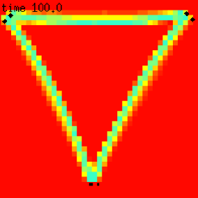
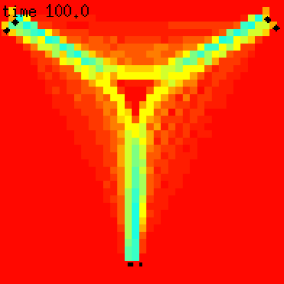
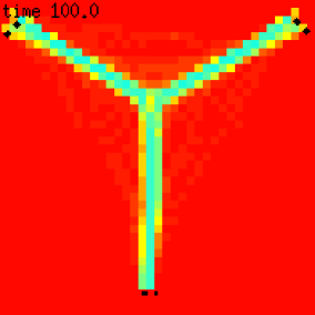
Figure 1b shows the result of computer simulations of trunk trail formation. The related dendritic trail system of Pheidole milicida, a harvesting ant of the southwestern U.S. deserts, is displayed in Figure 1a. In our simulation, a nest is assumed in the middle of a triangular lattice of size with periodic boundary conditions. Initially, there are no chemical markings on the lattice. At time , a number of walkers start from the nest with a random direction, leaving markings of chemical . If a walker disovers a food source by chance, it begins to produce chemical . Should such a walker find its way back to the nest, it activates an additional number of walkers, the recruits, to move out. The maximum number of walkers in the simulation is limited to , which denotes the population size.
For the food sources, an extended food distribution at the top and bottom line of the lattice is assumed [59]. These sources could be exhausted by the visiting walkers, but the accidental discovery of new ones in the neighborhood results in a branching of the main trails in the vicinity of the food sources and eventually leads to the dendritic structures. The trail system observed in Figure 1b remains unchanged in its major parts as has been reported also in the biological observations of trunk trail formation by ants [52]. Nevertheless, some minor trails in the vicinity of the food sources slightly shift in the course of time due to fluctuations.
IV Human trail formation
Trail formation by pedestrians has been investigated only very recently [60]. It can be interpreted as a complex interplay between pedestrian motion, human orientation, and environmental changes: On the one hand, pedestrians tend to take the shortest way to their destination. On the other hand, they avoid to walk on bumpy ground, since this is uncomfortable. Therefore, they prefer to use existing trails, but they build a new shortcut, if the relative detour would be too large. In the latter case they generate a new trail, since footprints clear some vegetation. Examples of the resulting trail systems can be found in green areas, like public parks (cf. Fig. 3).
Empirical studies have shown that pedestrian motion can be surprisingly well described by the social force model sketched in Section II [11, 29]. In particular, it has been demonstrated that this model allows a realistic simulation of various observed self-organization phenomena in pedestrian crowds [28, 29, 30, 31, 32, 33]. This includes the emergence of collective patterns of motion, e.g. lanes of uniform walking direction [30, 33] or roundabout traffic at intersections [31, 32, 33].
In this section, however, we want to model the evolution of human trail patterns. We will assume that the pedestrians behave ‘reasonably’ and, as before, we will restrict our model to the most important factors. It is obvious that pedestrians are able to show a much more complicated behavior than described here.
Since the equation (10) of motion can be also applied to pedestrians, we have to specify how moving pedestrians change their environment by leaving footprints, now. This time, we do not have to distinguish different kinds of markings. Thus, we will need only one ground potential , and the subscript can be omitted. The value of is a measure of the comfort of walking. (Therefore, it can considerably depend on the weather conditions, which is not discussed here any further.)
For the strength of the markings produced by footprints at place we assume
| (24) |
where is the location-dependent intensity of clearing vegetation. The saturation term results from the fact that the clarity of a trail is limited to a maximum value .
On a plain, homogeneous ground without any trails, the desired direction of a pedestrian at place is given by the direction of the next destination , i.e.
| (25) |
with the destination potential
| (26) |
However, the perception of already existing trails will have an attractive effect on the walker, which will again be defined by the gradient of the trail potential , specified later on:
| (27) |
Since the potentials and influence the pedestrian at the same time, it seems reasonable to introduce an orientation relation similar to (21), by taking the sum of both potentials:
| (28) | |||||
| (29) |
Here, serves as normalization factor. By relation (28) we reach that the vector points into a direction which is a compromise between the shortness of the direct way to the destination and the comfort of using an existing trail.
Finally, we need to specify the trail potential for pedestrians. Obviously a trail must be recognized by the walkers and near enough in order to be used. Whereas the ground potential describes the existence of a trail segment at position , the trail potential reflects the attractiveness of a trail from the actual position of the walker. Since this will decrease with the distance , we have applied the relation
| (30) |
where characterizes the sight, i.e. the range of visibility. In analogy to (15), this formula could be easily generalized to include conceivable effects of a pedestrian’s angle of sight. However, we will not do this here, since we would have to calculate different trail potentials for all walkers , then. This would make the model much more complicated.
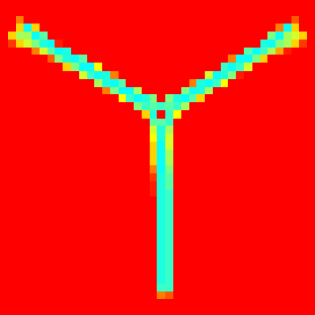
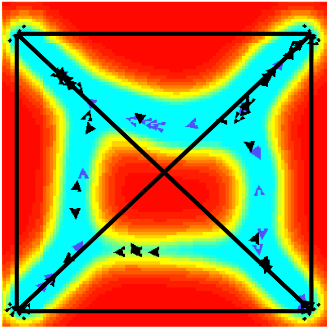
The simulation results of the above described trail formation model are in good agreement with empirical observations, as can be seen by comparison with photographs. Our multi agent simulations begin with plain, homogeneous ground. All pedestrians have their own destinations and entry points (like shops, houses, underground stations, or parking lots), from which they start at a randomly chosen time. In Figure 4 the entry points and destinations are distributed over the small ends of the ground, while in Figure 5 (Fig. 7) pedestrians move between all possible pairs of three (four) fixed places.
At the beginning, pedestrians take the direct ways to their respective destinations. However, after some time pedestrians begin to use already existing trails, since this is more comfortable than to clear new ways. The frequency of usage decides which trails are reinforced and which ones vanish in the course of time. If the attractiveness of the forming trails is large, the final trail system is a minimal way system (which is the shortest way system that connects all entry points and destinations). However, because of the pedestrians’ dislike of taking detours the evolution of the trail system normally stops before this state is reached. In other words, a so-called minimal detour system develops if the model parameters are chosen realistically (cf. Fig. 5). The resulting trails can considerably differ from the direct ways which the pedestrians would use if these were equally comfortable.
A Scaling to dimensionless equations
The use of existing trails depends on the visibility, as given by Eq. (30). Assuming that the sight parameter is approximately space-independent, an additional simplification of the equations of trail formation can be reached by introducing dimensionless variables
| (31) | |||||
| (32) | |||||
| (33) | |||||
| (34) | |||||
| (35) |
etc. Neglecting fluctuations in equation (10) for the moment, this implies the following scaled equations:
| (36) |
for pedestrian motion,
| (37) |
for human orientation, and
| (39) | |||||
for environmental changes. Therefore, we find the surprising result that the dynamics of trail formation is (apart from the influence of the number and places of entering and leaving pedestrians) already determined by two local parameters and instead of four, namely the products
| (40) |
and
| (41) |
Herein, denotes the mean value of the desired velocities .
B Macroscopic formulation of trail formation
From the above ‘microscopic’ model of trail formation we will now derive the related ‘macroscopic’ equations. For this purpose we need to distinguish different subpopulations of individuals . By we denote the time-dependent set of individuals who have started from the same entry point with the same destination . Therefore, the different sets correspond to the possible (directed) combinations between existing entry points and destinations.
Next, we define the density of individuals of subpopulation at place by
| (42) |
Note that a spatial smoothing of the density is reached by a discretization of space, which is needed for a numerical implementation of the model. For example, if the discrete places represent quadratic domains
| (43) |
with an area , the corresponding density is
| (44) |
However, for reasons of simplicity we will treat the continuous case.
The quantity
| (45) | |||||
| (46) |
describes the number of pedestrians of subpopulation , who are walking on the ground at time . It changes by pedestrians entering the system at the entry point with a rate and leaving it at the destinations with a rate .
Due to the time-dependence of the sets , we will need the set
| (47) |
of pedestrians remaining in the system, the set
| (48) |
of entering pedestrians, and the set
| (49) |
of leaving pedestrians, for which the following relations hold:
| (50) | |||||
| (51) | |||||
| (52) |
Therefore, equation (42) implies
| (54) | |||||
| (58) | |||||
Taking into account
| (60) | |||||
which follows by Taylor expansion, we obtain
| (64) | |||||
With
| (65) | |||||
| (66) | |||||
| (67) |
and the relations
| (68) | |||||
| (69) |
for the rates of pedestrians joining and leaving subpopulation , we finally arrive at
| (71) | |||||
where is zero away from the entry point , and the same holds for away from the destination .
Now, we define the average velocity by
| (72) |
This gives us the desired continuity equation
| (74) | |||||
describing pedestrian motion. Fluctuation effects can be taken into account by the additional diffusion terms
| (75) |
on the right-hand side of (74) [61, 28]. This causes the trails to become somewhat broader.
Next, we rewrite equation (39) for environmental changes in the form
| (77) | |||||
Finally, the orientation relation becomes
| (78) |
with
| (79) |
Therefore, the average velocity is given by
| (80) | |||||
| (81) |
where is again the average desired pedestrian velocity. In the case of frequent interactions (avoidance maneuvers) of pedestrians, must be replaced by suitable monotonically decreasing functions of the densities [28, 61, 62]. Moreover, fluctuation effects will be stronger, leading to greater diffusion functions and broader trails.
Summarizing our results, we have found a macroscopic formulation of trail formation which is given by equations (74) through (81) with (34). Apart from possible analytical investigations, it allows us to determine implicit equations for the stationary solution, if the rates and are time-independent. Setting the temporal derivatives to zero, we find the relations
| (82) |
and
| (83) |
Together with equations (34) and (78) through (81), relations (82) and (83) allow to calculate the finally evolving trail system. Again, we see that the resulting state depends on the two parameters and . In addition, it is determined by the respective boundary conditions, i.e. the configuration and frequency of usage of the entry point-destination pairs, which are characterized by the concrete form of the entering rates and leaving rates .
The advantage of applying the macroscopic equations is that the finally evolving trail system can be calculated much more efficiently, since considerably less time is required for computing: The numerical solution can now be obtained by means of a simple iterative method which is comparable to the self-consistent field technique. Examples are shown in Figure 6 for different values of . As expected, the results agree with the ones of the related microsimulations, which are depicted in Figure 5.
V Summary and Outlook
We showed that the active walker concept is suitable for modeling and understanding trail formation by pedestrians and animals. Our model turned out to be in good agreement with observations. It included an equation of motion of the walkers, an equation describing environmental changes by the markings which they leave and their decay, a relation reflecting the attractiveness of already existing trails, and an equation delineating their influence on orientation. Whereas frequently used trails are reinforced, rarely chosen trails are vanishing in the course of time. This causes a tendency of trail bundling, which can be interpreted as an agglomeration phenomenon. However, the evolving patterns are not localized since the active walkers intend to reach certain destinations, starting from their respective entry points.
The structure of the resulting trail system can considerably vary with the species. This depends decisively on the main effect which counteracts the trail attraction. Whereas our model ants find their destinations (the food sources) by chance, pedestrians can directly orient towards their destinations, so that fluctuations are no necessary model component in this case. Thus, for certain ant species a dendritic trail system is found, the detailed form of which depends on random events, i.e. the concrete history of its evolution. Pedestrians, however, produce a minimal detour system, i.e. an optimal compromise between a direct way system and a minimal way system.
As a consequence, we could derive a macroscopic model for the trail formation by pedestrians, but not for ants. It implied a self-consistent field method for a very efficient calculation of the finally evolving trail system. This is determined by the location of the entry points and destinations (e.g. houses, shops, or parking lots) and the rates of choosing the possible connections between them. Apart from this it depends on two parameters only, which was demonstrated by scaling to dimensionless equations. These are related to the trail attractiveness and the average velocity of motion.
A Trail formation as a self-organization phenomenon
In order to demonstrate that the evolution of trail systems can be understood as a typical self-organization phenomenon, our model has made a number of simplifying assumptions about the agents.
In the example of trail formation by certain ant species, the major difference to biology is, that the active walkers used in the simulations have far less complex capabilities than the biological creatures. They almost behave like physical particles which respond to local forces in a quite simple manner, without “implicit and explicit intelligence” [56]. Compared to the complex ‘individual-based’ models in ecology [8], the active walker model proposed here provides a very simple but efficient tool to simulate a specific structure only with a few adjustable parameters.
With respect to the formation of trunk trails, our model indicates that these patterns can be obtained also under the restrictions, that (i) no visual navigation and internal storage of information is provided, (ii) in the beginning, no chemical signposts exist which lead the ants to the food sources and afterwards back to the nest. Rather, the formation of trail systems can be described as a process of self-organization. Based on the interactions of the active walkers on a local or ‘microscopic’ level, the emergence of a global or ‘macroscopic’ structure occurs. The basic interaction between the active walkers can be considered as indirect communication mediated by an external storage medium [43, 63]. This is a collective process in which all active walkers are involved. The information which an active walker produces in terms of chemical markings affects the behaviors of the others. It can be amplified during the evolution process or disappear again, thus leading to a correlation between the information generated and to the self-organization of the walkers on a spatial level.
B Implications for urban planners: Optimization of way systems
Computer simulations of our pedestrian trail formation model will be a valuable tool for designing convenient way systems (cf. Fig. 7). For planning purposes the model parameters and must be specified in a realistic way. Then, one needs to simulate the exptected flows of pedestrians that enter the considered system at certain entry points with the intention to reach certain destinations. Already existing ways can be taken into account by the function . According to our model, a trail system will evolve which minimizes overall detours and thereby provides an optimal compromise between a direct and a minimal way system. It is expected that the corresponding ways meet the pedestrian requirements best: They will most likely be accepted and actually used, since they take into account the route choice habits of pedestrians. For the simulation of realistic situations, the results can serve as planning guidelines for architects, landscape gardeners, and urban planners.
C Current research directions
Besides of possible applications, our present research focusses on two questions: (i) How must our trail formation model be specified in order to be applicable to trail formation by hoofed animals or mice [64, 65]? (ii) Can our model be generalized in a way that allows to understand human decision making, in particular processes of finding suitable compromises? Interestingly enough, one says that someone “follows in somebody’s footsteps” or that someone “treads new paths”. Therefore, a related theory for a more abstract space (which represents the set of behavioral alternatives) may describe the evolution of social norms and conventions [11].
REFERENCES
- [1] H. Haken, Synergetics. An Introduction (Springer, Berlin, 3rd ed., 1987).
- [2] H. Haken, Advanced Synergetics (Springer, Berlin, 2nd ed., 1987).
- [3] G. Nicolis and I. Prigogine, Self-Organization in Nonequilibrium Systems. From Dissipative Structures to Order through Fluctuations (Wiley, New York, 1977).
- [4] R. Feistel and W. Ebeling, Evolution of Complex Systems. Self-Organization, Entropy and Development (Kluwer, Dordrecht, 1989).
- [5] S. Kai (ed.) Pattern Formation in Complex Dissipative Systems (World Scientific, Singapore, 1992).
- [6] P. E. Cladis and P. Palffy-Muhoray (eds.) Spatio-Temporal Patterns in Nonequilibrium Complex Systems (Addison-Wesley, Reading, MA, 1995).
- [7] J. M. Pasteels and J. L. Deneubourg (eds.) From Individual to Collective Behavior in Social Insects (Birkhäuser, Basel, 1987).
- [8] D. L. DeAngelis and L. J. Gross (eds.) Individual-Based Models and Approaches in Ecology: Populations, Communities, and Ecosystems (Chapman and Hall, New York, 1992).
- [9] R. Vallacher and A. Nowak (eds.) Dynamic Systems in Social Psychology (Academic Press, New York, 1994).
- [10] W. Weidlich, Physics Reports 204, 1 (1991).
- [11] D. Helbing, Quantitative Sociodynamics. Stochastic Methods and Social Interaction Processes (Kluwer Academic, Dordrecht, 1995).
- [12] R. Axelrod and D. Dion, Science 242, 1385 (1988).
- [13] S. H. Clearwater, B. A. Huberman, and T. Hogg, Science 254, 1181 (1991).
- [14] E. W. Montroll and W. W. Badger, Introduction to Quantitative Aspects of Social Phenomena (Gordon and Breach, New York, 1974).
- [15] K. Nagel and M. Paczuski, Phys. Rev. E 51, 2909 (1995).
- [16] M. Schreckenberg, A. Schadschneider, K. Nagel, and N. Ito, Phys. Rev. E 51, 2939 (1995).
- [17] K. Nagel and H. J. Herrmann, Physica A 199, 254 (1993).
- [18] K. Nagel and S. Rasmussen, in Proceedings of the Alife 4 meeting, edited by R. Brooks and P. Maes (MIT Press, Cambridge, MA, 1994).
- [19] M. Bando, K. Hasebe, A. Nakayama, A. Shibata, and Y. Sugiyama, Phys. Rev. E 51, 1035 (1995).
- [20] T. S. Komatsu and S.-i. Sasa, Phys. Rev. E 52, 5574 (1995).
- [21] O. Biham, A. A. Middleton, and D. Levine, Phys. Rev. E 46, R6124 (1992).
- [22] J. A. Cuesta, F. C. Martínez, J. M. Molera, and A. Sánchez, Phys. Rev. E 48, R4175 (1993).
- [23] J. M. Molera, F. C. Martínez, J. A. Cuesta, and R. Brito, Phys. Rev. E 51, 175 (1995).
- [24] T. Nagatani, Phys. Rev. E 48, 3290 (1993).
- [25] T. Nagatani, Phys. Rev. E 51, 922 (1995).
- [26] E. Ben-Naim, P. L. Krapivsky, and S. Redner, Phys. Rev. E 50, 822 (1994).
- [27] I. Campos, A. Tarancón, F. Clérot, and L. A. Fernández, Phys. Rev. E 52, 5946 (1995).
- [28] D. Helbing, Verkehrsdynamik. Neue physikalische Modellierungskonzepte (Springer, Berlin, 1997).
- [29] D. Helbing, Behavioral Science 36, 298 (1991).
- [30] D. Helbing and P. Molnár, Phys. Rev. E 51, 4282 (1995).
- [31] D. Helbing, in Traffic and Granular Flow, edited by D. E. Wolf, M. Schreckenberg, and A. Bachem (World Scientific, Singapore, 1996).
- [32] D. Helbing and P. Molnár, in Self-Organization of Complex Structures: From Individual to Collective Dynamics, edited by F. Schweitzer (Gordon and Breach, London, 1997).
- [33] D. Helbing, P. Molnár, and F. Schweitzer, in Evolution of Natural Structures (Sonderforschungsbereich 230, Stuttgart, 1994).
- [34] D. Helbing, J. Keltsch, and P. Molnár, Nature 388, 47 (1997).
- [35] F. Schweitzer, in Prozeß und Form natürlicher Konstruktionen, edited by K. Teichmann and J. Wilke (Ernst&Sohn, Berlin, 1996).
- [36] B. Davis, Probab. Th. Rel. Fields 84, 203 (1990).
- [37] R. D. Freimuth and L. Lam, in Modeling Complex Phenomena, edited by L. Lam and V. Naroditsky (Springer, New York, 1992).
- [38] D. R. Kayser, L. K. Aberle, R. D. Pochy, and L. Lam, Physica A 191, 17 (1992).
- [39] R. D. Pochy, D. R. Kayser, L. K. Aberle, and L. Lam, Physica D 66, 166 (1993).
- [40] L. Lam and R. Pochy, Computers in Physics 7, 534 (1993).
- [41] L. Lam, Chaos, Solitons & Fractals 6, 267 (1995).
- [42] F. Schweitzer, in Lectures on Stochastic Dynamics, edited by L. Schimansky-Geier and T. Pöschel (Springer, Berlin, 1997).
- [43] F. Schweitzer and L. Schimansky-Geier, Physica A 206, 359 (1994).
- [44] L. Schimansky-Geier, M. Mieth, H. Rosé, and H. Malchow, Physics Letters A 207, 140 (1995).
- [45] L. Schimansky-Geier, F. Schweitzer, and M. Mieth, in Self-Organization of Complex Structures: From Individual to Collective Dynamics, edited by F. Schweitzer (Gordon and Breach, London, 1997).
- [46] F. Schweitzer and L. Schimansky-Geier, in Fluctuations and Order: The New Synthesis, edited by M. Millonas (Springer, New York, 1996).
- [47] A. Stevens, Mathematical Modeling and Simulations of the Aggregation of Myxobacteria (PhD thesis, Ruprecht-Karls-University Heidelberg, 1992).
- [48] A. Stevens and F. Schweitzer, in Dynamics of Cell and Tissue Motion, ed. by W. Alt, A. Deutsch, and G. Dunn (Birkhäuser, Basel, 1997).
- [49] F. Schweitzer and J. Steinbrink: in: Self-Organization of Complex Structures: From Individual to Collective Dynamics, edited by F. Schweitzer (Gordon and Breach, London, 1997).
- [50] W. Ebeling, F. Schweitzer, B. Tilch, and V. Calenbuhr, submitted to J. Mathem. Biol. (1995).
- [51] F. Schweitzer, K. Lao, and F. Family, BioSystems 41, 153 (1997).
- [52] B. Hölldobler and M. Möglich, Insectes Sociaux 27, 237 (1980).
- [53] B. Hölldobler and E. O. Wilson, The Ants (Belknap, Cambridge, MA, 1990).
- [54] J. L. Deneubourg, S. Goss, N. Franks, and J. M. Pasteels, J. Insect Behavior 2(5), 719 (1989).
- [55] R. Wehner, in: Animal Homing, edited by F. Papi (Chapman and Hall, London, 1992).
- [56] J. W. Haefner and T. O. Crist, J. theor. Biol. 166, 299 (1994).
- [57] F. Schweitzer and B. Tilch, “Network formation with Active Brownian Particles”, in preparation (1997).
- [58] W. Alt, J. Math. Biol. 9, 147 (1980).
- [59] For the simulation of different source distributions cf. [51].
- [60] M. Schenk, Untersuchungen zum Fußgängerverhalten (PhD thesis, University of Stuttgart, 1995).
- [61] D. Helbing and A. Greiner, “Modeling and simulation of multi-lane traffic flow”, Phys. Rev. E 55, 5498 (1997).
- [62] D. Helbing, Complex Systems 6, 391 (1992).
- [63] F. Schweitzer, Word Futures: The Journal of General Evolution, in print (1997)
- [64] E. Schaur, Non-Planned Settlements (Institute for Lightweight Structures, Stuttgart, 1991).
- [65] F. Otto, Die natürliche Konstruktion gewachsener Siedlungen (Sonderforschungsbereich 230, Stuttgart, 1991).
Acknowledgments
The authors would like to thank K. Humpert and B. Hölldobler for providing some of their interesting (photo)graphical material.