Liquid State Anomalies for the
Stell-Hemmer Core-Softened Potential

Abstract

We study the Stell-Hemmer potential using both analytic (exact $1d$ and approximate $2d$) solutions and numerical $2d$ simulations. We observe in the liquid phase an anomalous decrease in specific volume and isothermal compressibility upon heating, and an anomalous increase in the diffusion coefficient with pressure. We relate the anomalies to the existence of two different local structures in the liquid phase. Our results are consistent with the possibility of a low temperature/high pressure liquid-liquid phase transition.

ssbs.tex     May 15, 1998     draft

PACS numbers: 61.20.Gy, 61.25.Em, 65.70.+y, 64.70.Ja

In their pioneering work, Stell and Hemmer proposed the possibility of a new critical point in addition to the normal liquid-gas critical point for potentials that have a region of negative curvature in their repulsive core (henceforth referred to as core-softened potentials) [1]. They also pointed out that for the $1d$ model with a long long range attractive tail, the isobaric thermal expansion coefficient, $\alpha_{P}\equiv V^{-1}\left(\partial V/\partial T\right)_{P}$ (where $V,T$ and $P$ are the volume, temperature and pressure) can take an anomalous negative value. Debenedetti et al., using thermodynamic arguments, pointed out that the existence of a “softened core” can lead to $\alpha_{P}<0$ [2].

Here we further investigate properties of core-softened potential fluids. We first study the properties of the $1D$ fluid using an exact solution. We then investigate the behavior of the $2D$ fluid, initially by an approximate solution provided by cell theory method and finally by performing molecular dynamics simulation of the fluid.

The discrete form of the potential that we study is

$$u(r)\equiv\left\{\begin{array}[]{ll}\infty&0<r<a\\ -\lambda\epsilon&a<r<b\\ -\epsilon&b<r<c\\ 0&r>c\end{array}\right.$$ (1)

with $r$ being the inter-particle distance and $\lambda<1$ (Fig. 1(a)) [3]. The model is exactly solvable in $1d$, following the methods of [4, 5, 6, 7], and the equation of state is

$\underline{|\hskip 247.53888pt}$

$$V(T,P)/N=a+\frac{1}{P}\left(k_{B}T+\frac{P\left[(b-a)(1-W^{\lambda})\Pi_{b}+\left((b-a)\Pi_{b}-(c-a)\Pi_{c}\right)(W-1)\right]}{\Pi_{a}W^{\lambda}+\Pi_{b}(1-W^{\lambda})+(\Pi_{b}-\Pi_{c})(W-1)}\right).$$ (2)

$\overline{|\hskip 247.53888pt}$

Here $V/N\equiv\ell$ is the average distance between nearest neighbors, $\Pi_{x}\equiv e^{-\beta Px}$ ($x=a,b,c$), $W\equiv e^{\beta\epsilon}$ and $\beta\equiv k_{B}T$. The isobars (Fig. 1(b)) exhibit two different types of behavior. For all $P$ larger or equal to an upper boundary pressure $P_{up}$, $\ell=a$ at $T=0$, and $\ell$ increases monotonically with $T$. For $P<P_{up}$, $\ell=b$ at $T=0$. The isobars show a maximum and a minimum in $\ell$, which correspond respectively to points of minimum and maximum density[8], bounding a density anomaly ($\alpha_{P}<0$) region [9, 10]. There is a discontinuity in $\ell$ at $P=P_{up}$ along the $T=0$ isotherm.

Next we study the isothermal compressibility $K_{T}\equiv-V^{-1}\left({\partial V/\partial P}\right)_{T,N}$. We use Eq.(2) to calculate $K_{T}$ along isobars (Fig. 1(c)). The graphs show an anomalous region in which $K_{T}$ decreases upon heating (for simple liquids $K_{T}$ increases with $T$). We find the maximum value of $K_{T}$ grows as $P$ increases towards $P_{up}$, and $K_{T}$ diverges as $1/T$ when we approach the point $C^{\prime}$ with coordinates $(T=0,P=P_{up})$ which we interpret as a critical point [11]. Further, the locus of $K_{T}$ extrema joins the point $C^{\prime}$(Fig. 1(d)).

We also study the $T_{MD}$ locus (Fig. 1(d)) and note that the locus of $K_{T}$ extrema intersects the $T_{MD}$ locus at its infinite slope point, a result that is thermodynamically required[12]. Such a point on the $T_{MD}$ has been observed in simulations which support the existence of a liquid-liquid phase transition in supercooled water [13].

We next consider the $2d$ case, for which an exact solution does not exist. We use the spherical Lennard-Jones and Devonshire cell theory method[15] which assumes that each particle is confined to a circular cell, whose radius is determined by the average area per particle, $v$. This method neglects the correlation between the positions of different particles and assumes that the potential acting on each particle is a result of interacting with all its nearest neighbors smeared around its cell. The Helmholtz free energy per cell is

$$h(v,T)=h_{i}(v,T)-k_{B}T\ln(v_{f}(v,T)/v),$$ (3)

where $h_{i}(v,T)$ is the ideal gas free energy and $v_{f}(v,T)$ is the free volume defined as

$$v_{f}(v,T)\equiv\int_{\mbox{cell}}e^{-\beta u(x)}d\mbox{\bf x}$$ (4)

with the core-softened potential used for $u(\mbox{\bf x})$ . For each value $(P,T)$, we find the value of $v(P,T)$ by minimizing $h(v,T)-Pv$. The resulting phase diagram (Fig. 2) has two lines of first order phase transition, a low pressure line which is the liquid-gas phase transition line terminating at a critical point $C$, and a high pressure line that separates a low-density liquid (LDL) and a high-density liquid (HDL) and terminates in a critical point $C^{\prime}$. This picture holds both for the discrete and smooth versions of the potential. We note that the presence of $C^{\prime}$ would imply an anomalous increase in $K_{T}$ upon cooling when $C^{\prime}$ is approached from higher temperatures.

In order to further investigate the system in the liquid phase we rely on numerical molecular dynamics (MD) study of the discrete and smooth versions of the potential (Fig. 1(a)). We perform $2d$ MD simulations for a system composed of $N$ circular disks, in a rectangular box of area $A$. To each disk we assign a radius equal to half the hard core diameter $a$, and define the density $\rho$ as the ratio of the total area of all the disks to the area of the box. For the discrete version of the potential we use the collision table technique [16] for $N=896$ disks and for the smooth version of the potential, we use the velocity Verlet integrator method [16] with $N=2500$. We set the mass of the particles to be unity, while the units of length and energy are scaled by $\epsilon$ and $a$ respectively. We choose the time step $\delta t=0.01$ [17]. For each $T$, we first slowly thermalize the system, using the Berendsen method of rescaling the kinetic energy [16], after which we perform the simulation at constant $N,A$ and energy $E$. We fix $\rho$ by fixing $A$ and we start from $T=1$, lowering $T$ down to $0.4$ (in steps of $\Delta T=0.1$ for larger $T$ and $\Delta T=0.05$ and $0.025$ in the vicinity of freezing). As the initial configuration for each $(\rho,T)$, we choose the equilibrated configuration of $(\rho,T+\Delta T)$. We simulate state points along constant $\rho$ paths (isochores) (Fig. 3(a)) and also along constant $P$ paths (isobars) [19]. We use the isobar results to check the values of $\rho(T,P)$ calculated from isochores, as well as to find $K_{T}$ along isobars (Fig. 3(b)) [20].

The MD results are qualitatively equivalent for the discrete and smooth versions of the potential. For the results of Fig. 3 we have used the smooth version. The minima in the $P$ versus $T$ isochores (Fig. 3(a)) correspond to density maximum points [18]. We also find that along some of the isobars, $K_{T}$ increases upon cooling (Fig. 3(b)) [21]. The $T_{MD}$ locus possesses a point with infinite slope (as in $1d$), which we verify by finding the intersection of the locus of $K_{T}$ minima with the $T_{MD}$ line in Fig. 3(a)[12]. If we assume that a metastable liquid critical point exists below freezing, then by fitting the $K_{T}$ graph to a power law divergence, we can estimate the critical point to be in the region $0.3<T<0.5$ and $1.0<P<1.5$ which is in agreement with the cell-theory approximation.

We also study the effect of pressure on diffusion, and find that along some isotherms, increasing pressure increases $D$, while for simple liquids increasing pressure decreases $D$ (Fig. 3(c)). This anomaly occurs in the same region of phase diagram where the density and isothermal compressibility anomaly is observed.

The anomalies can be related to the interplay between two local structures, an open structure in which the nearest neighbor particles are typically at a distance $b$ and a denser structure in which the nearest neighbors penetrate into the softened core and are typically at a smaller distance $a$. The configurations are determined by the minima of the Gibbs free energy, $G(T,P)=U+PV-TS$ (where $G,U$ and $S$ are the Gibbs free energy, internal energy, and entropy). Fig. 4(a) shows the 1d free energy at $T=0$ for two different values of $P$. The qualitative shape should not change for higher dimensions and small $T$. For low pressures at small $T$, the open structure is favored by the free energy. Increasing $T$ for these pressures will increase local fluctuations in the form of dense structures which can lead to an overall contraction of the system upon heating, causing a density anomaly. Increasing $P$ raises the relative free energy of the open structure, until the dense structure will be the favored local structure, as seen for $P>P_{up}$ in Fig. 4(a). At small $T$ this can lead to a first order pressure driven transition (“core-collapse”[1]), while for large $T$ the transition is continuous. At $T=0$, the value of $P_{up}$ where the transition occurs is where $G(T=0,P)$ is the same for the open and dense structures, so

$$P_{up}=-\frac{U_{open}-U_{dense}}{V_{open}-V_{dense}}.$$ (5)

From Eq.(1) and Eq.(5) we find $P_{up}={(1-\lambda)\epsilon/(b-a)}$ in 1d, which can also be derived from Eq.(2)[14].

To examine the transition from the open structure to dense structure in $2d$, we study the pair distribution function $g(r)$ for the MD configurations (Fig. 4(b)). The first peak in $g(r)$ splits into two subpeaks, which correspond to the locations of the nearest neighbors in the dense and open structures. As $T$ increases, the open structure subpeak decreases while the dense structure subpeak increases. We observe the same change with $P$ along the liquid isotherms for small $T$. The uniform value of $g(r)$ for large $r$ confirms that all the state points of Fig. 3(a) are in the liquid state.

We thank M. Canpolat, S. Havlin, B. Kutnjak-Urbanc, M. Meyer, S. Sastry, A. Skibinsky, F. Starr, G. Stell and D. Wolf for helpful discussions, NSF for financial support.

 

 

FIG. 1.: (a) General form for the core-softened potential studied here. The length parameters $a,b,c$ and energy parameters $\epsilon,\lambda$ are shown. The dashed curve is the smooth version [3]. (b) Isobars (the average distance per particle, $\ell$ versus $T$ at constant $P$) for the discrete $1d$ core-softened potential[3] with $P_{up}=2.5$ in agreement with Eq.(5). The $T_{MD}$ point is marked by an open circle. (c) Isothermal compressibility for the discrete potential along different isobars, with their maxima marked by filled circles. The $K_{T}$ for $P_{up}$ diverges as $1/T$. (d) The loci of $T_{MD}$ and $K_{T}$ extrema for the discrete potential.

 

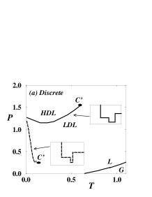
FIG. 2.: (a) Solid lines correspond to the phase diagram from the cell theory method for the $2d$ discrete potential with the same parameters as in Fig. 1 (solid curve inset). The lower solid line corresponds to the liquid-gas (L-G) phase transition, with a critical point outside the range of the graph. The upper solid line corresponds to the HDL to LDL phase transition, the slope of which changes from negative to positive. The Clausius-Clapeyron equation relates the slope of a first order transition line to the difference between the entropy and volume of the phases by $dP/dT=\Delta S/\Delta V$. In the case of water, the open LDL structure produced by highly directional hydrogen bonding has a lower entropy. We can mimic this situation for our radially symmetric potential by narrowing the well which greatly reduces the positively sloped part of the transition line; the dashed line corresponds to the HDL-LDL transition for a discrete potential with $c=1.40001$. (b) Similar phase diagrams for the smooth version of the potential in Fig. 1(a)(solid lines). The dashed line correspond to a potential with a much narrower well ($w=10,000$).

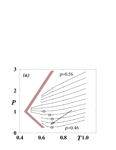
FIG. 3.: MD results for the smooth potential with the same parameters as in Fig. 1[3]. (a) Constant density curves with, from bottom to top, densities between $0.46$ to $0.56$ in steps of $0.1$. The open circles mark $T_{MD}$ and the dashed line is the locus of $K_{T}$ minima from part (b). The thick gray line is the approximate locus of the freezing points. (b) Isothermal compressibility along isobars. Except for the $P=0.25$ isobar, the graphs show anomalous decrease upon heating. (c) Diffusion coefficient $D$ (slope of the mean square displacement as a function of time) for different pressures at $T=0.65$, showing an anomalous increase in the $P<1.5$ range. For comparison, we show $D/4$ for a Lennard-Jones liquid at $T=0.7$, from simulation of $2304$ disks. The high pressure zero values in both graphs correspond to a solid phase.

 

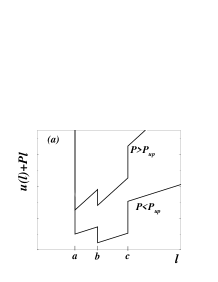
FIG. 4.: (a) The 1d Gibbs free energy at $T=0$ as a function of the extra “degree of freedom” $\ell$, for the discrete form of potential in Fig. 1(a). The equilibrium value of $\ell(P)$ is determined as the absolute minimum of this function, which is located at $\ell=b$ below $P_{up}$ and at $\ell=a$ above $P_{up}$. (b) Pair distribution function for $T=0.6$ and $T=1.0$ on the $\rho=0.48$ isochore of Fig. 3(a). The uniform $g(r)$ for large $r$ is a sign of the liquid phase. The inset is a blow up of the first (split) peak. The thick solid curve is for $T=1.0$ and the dashed curve is for $T=0.6$, indicating that increasing $T$ lowers the total number of particles in the open structure ($r\approx 1.5$) and increases the number of particles in the dense structure ($r\approx 1.1$).

REFERENCES

- [1] P. C. Hemmer and G. Stell, Phys. Rev. Lett. 24, 1284 (1970); G. Stell and P. C. Hemmer, J. Chem. Phys. 56, 4274 (1972); J. M. Kincaid, G. Stell and C. K. Hall, ibid, 65, 2161 (1976); J. M. Kincaid, G. Stell and E. Goldmark, ibid, 65, 2172 (1976).
- [2] P. G. Debenedetti et al., J. Phys. Chem. 95, 4540 (1991).
- [3] We also use a smooth form of the potential with the form . Unless stated otherwise, all of the results reported here are for a discrete potential with , , , , and and its smooth version with , , , , (Fig. 1(a)).
- [4] H. Takahashi, Proc. Phys. Math. Soc. Japan, 24, 60 (1942); Mathematical Physics in One Dimension, edited by E. H. Lieb and D. C. Mattis (Academic, New York, 1966) pp. 25-34.
- [5] Y. Yoshimura, Ber. Bunsenges. Phys. Chem. 95, 135 (1991).
- [6] A. Ben-Naim, Statistical Thermodynamics for Chemists and Biochemists (Plenum, New York, 1992).
- [7] C. H. Cho et al., Phys. Rev. Lett. 76, 1651 (1996).
- [8] We focus attention on the maximum density point, which is located at a higher temperature and has been observed in several real materials, including liquid water, and in simulations[13]. To our best knowledge, the minimum density point has only been observed for the liquid tellurium alloy with selenium (See [5] and references therein). In this phase diagram, in addition to the the upper bound , there is a lower bound where the locus of density maxima ( line) terminates by joining the locus of density minima. Below this lower bound the isobars do not show a density anomaly.
- [9] Similar behavior of isobars has been previously reported for two-state lattice models [10]. Also the existence of the maximum density point for in has been reported for a double well potential (in which the potential has a barrier between the two energy states[7]). The double well form of the potential, because of its region of negative curvature, belongs to the general category of core-softened potentials.
- [10] G. M. Bell and H. Sallouta, Mol. Phys. 29, 1621 (1975).
- [11] For the Stell-Hemmer potential with a long-range attractive tail added, the line of first order transitions extends up to a critical point. For our short-range potential, there cannot exist any critical point for .
- [12] S. Sastry et al., Phys. Rev. E 53, 6144 (1996).
- [13] P. H. Poole et al., Nature 360, 324 (1992); Phys. Rev. E 48, 3799 (1993); S. Harrington et al, Phys. Rev. Lett. 78, 2409 (1997); J. Chem. Phys. 107, 7443 (1997).
- [14] In higher dimensions, Eq.(5) helps estimating the pressure region in which we expect to observe the anomalies.
- [15] J. E. Lennard-Jones and A. F. Devonshire, Proc. R. Soc. London, Ser. A 163, 53 (1937);165, 53 (1938); 169, 53 (1939);170, 53 (1939).
- [16] M. P. Allen and D. J. Tildesley, Computer Simulation of Liquids (Oxford University Press, New York, 1989).
- [17] For the continuous potential the average simulation speed on Boston University’s SGI origin2000 supercomputer cluster was approximately per particle update on a single processor run and between half to one third of this for parallel runs on or processors. For the discrete potential the average speed is around per collision on an alpha Dec station.
- [18] Since , a minimum along the isochore implies .
- [19] For the isobars, in addition to thermalizing, we achieve a preset by rescaling the particle positions and the box size every time steps, using the value of the virial and its derivative [J. Q. Broughton et al., J. Chem. Phys. 75, 5128 (1981)].
- [20] We calculate using , where the structure function is the Fourier transform of the pair distribution function . We also use the relation , where and are average number density and its variance averaged over boxes of edges equal to of system edges. The results of the two methods agree.
- [21] We also simulated the double well version of the core-softened potential, in which there is an energy barrier between the two energy states. Our results did not show a density anomaly, in accord with a recent study that casts doubt on the ability of the double well version of the core-softened potential to show a in its liquid phase in [E. Velasco et al., Phys. Rev. Lett. 79, 179 (1997)].