Mutual Information of Sparsely Coded Associative Memory with Self-Control and Ternary Neurons

Abstract

Abstract

The influence of a macroscopic time-dependent threshold on the retrieval dynamics of attractor associative memory models with ternary neurons $\{-1,0.+1\}$ is examined. If the threshold is chosen appropriately in function of the cross-talk noise and of the activity of the memorized patterns in the model, adapting itself in the course of the time evolution, it guarantees an autonomous functioning of the model. Especially in the limit of sparse coding, it is found that this self-control mechanism considerably improves the quality of the fixed-point retrieval dynamics, in particular the storage capacity, the basins of attraction and the information content. The mutual information is shown to be the relevant parameter to study the retrieval quality of such sparsely coded models. Numerical results confirm these observations.

Keywords: Associative memory; Ternary neurons; Sparse coding; Self-control dynamics; Mutual information; Storage capacity; Basin of attraction.

1. Introduction

An important property required in efficient neural network modelling is an autonomous functioning independent from, e.g., external constraints or control mechanisms. For fixed-point retrieval by an attractor associative memory model this requirement is mainly expressed by the robustness of its learning and retrieval capabilities against external noise, against malfunctioning of some of the connections and so on. Indeed, a model which embodies this robustness is able to perform as a content-adressable memory having large basins of attraction for the memorized patterns. Intuitively one can imagine that these basins of attraction become smaller when the storage capacity gets larger. This might occur, e.g., in sparsely coded models (Okada, 1996 and references cited therein). Therefore the necessity of a control of the activity of the neurons has been emphasized such that the latter stays the same as the activity of the memorized patterns during the recall process. In particular, for binary patterns with a strong bias some external constraints were proposed on the dynamics in order to realize this (Amit et al., 1987; Amari,1989; Buhman et al., 1989; Schwenker et al., 1996).

An interesting question is then whether the recall process can be optimized without imposing such external constraints, keeping the simplicity of the (given) architecture of the network model. To this end a self-control mechanism has been proposed in the dynamics of binary neuron models through the introduction of a time-dependent threshold in the transfer function. This threshold is determined in function of both the cross-talk noise and the activity of the memorized patterns in the network and adapts itself in the course of the time evolution (Dominguez and Bollé, 1998).

The purpose of the present paper is to derive and verify this self-control mechanism for attractor networks with multi-state neurons. There are obvious reasons for choosing multi-state (or even analog) neurons in device oriented applications of neural networks. To give one example, the pixels of a colored or gray-toned pattern are represented by such neurons. In the sequel we restrict ourselves, for convenience and without loss of generality, to ternary neurons $\{-1,0,+1\}$. Although the dynamics and the interesting features of the latter have been discussed (see, e.g., Yedidia, 1989; Bouten and Engel, 1993; Bollé et al., 1994 and references therein) especially in the limit of small pattern activity (Yedidia, 1989), no activity control mechanism has been proposed in the literature until now.

The rest of this paper is organized as follows. In Section 2 we define the attractor associative memory network model with ternary neurons and we introduce the relevant parameters in order to discuss the quality of the recall process. Section 3 introduces the mutual information function for this model and discusses an explicit analytic expression for it. In Section 4 we study the fixed-point retrieval dynamics of the model with complete self-control. In particular, using a probabilistic signal-to-noise approach we obtain explicit time evolution equations and we consider the consequences of sparse coding. Section 5 studies the numerical solutions of this self-controlled dynamics and compares the quality of the recall process in this case with the one for models without self-control. Numerical simulations are shortly discussed. Finally, in Section 6 we present some concluding remarks.

2. The model

Let us consider a network with $N$ ternary neurons. At a discrete time step $t$ the neurons $\sigma_{i,t}\in\{0,\pm 1\},i=1,\ldots,N$ are updated synchronously according to the rule

$$\sigma_{i,t+1}=F_{\theta_{t}}(h_{i,t}),\quad h_{i,t}=\sum_{j(\neq i)}^{N}J_{ij}\sigma_{j,t},$$ (1)

where $h_{i,t}$ is usually called the “local field” (Hertz et al., 1991) of neuron $i$ at time $t$. In general, the transfer function $F_{\theta_{t}}$ can be a monotonic function with $\theta_{t}$ a time-dependent threshold parameter. Later on it will be chosen as

$$F_{\theta_{t}}(x)=\cases{\mbox{sign}(x)&\mbox{if $|x|>\theta_{t}$}\cr 0&\mbox{if $|x|<\theta_{t}$}\, .}$$ (2)

In the sequel, for theoretical simplicity in the methods used, the number of neurons $N$ will be taken to be sufficiently large.

The synaptic weights $J_{ij}$ are determined as a function of the memorized patterns $\xi^{\mu}_{i}\in\{0,\pm 1\},i=1,\ldots,N,\mu=1,\ldots,p$, by the following learning algorithm

$$J_{ij}={C_{ij}\over Ca}NJ_{ij}^{H},\quad J_{ij}^{H}=\frac{1}{N}\sum_{\mu=1}^{p}\xi^{\mu}_{i}\xi^{\mu}_{j}.$$ (3)

In this learning rule the $J_{ij}^{H}$ are the standard Hebb weights (Hebb, 1949; Hertz et al., 1991) with the ternary patterns $\xi^{\mu}_{i}$ taken to be independent identically distributed random variables (IIDRV) chosen according to the probability distribution

$$p(\xi^{\mu}_{i})=a\delta(|\xi^{\mu}_{i}|^{2}-1)+(1-a)\delta(\xi^{\mu}_{i}).$$ (4)

Here $a=\langle|\xi^{\mu}_{i}|^{2}\rangle$ is the $activity$ of the memorized patterns which is taken to be the same for all $\mu$ and which is given by the limit $N\rightarrow\infty$ of

$$a^{\mu}_{N}\equiv{1\over N}\sum_{i}|\xi_{i}^{\mu}|^{2}.$$ (5)

The brackets $\langle\cdots\rangle$ denote the average over the memorized patterns. The latter are unbiased and uncorrelated, i.e., $\langle\xi^{\mu}_{i}\rangle=0,\langle\xi^{\mu}_{i}\xi^{\nu}_{i}\rangle=0$. To obtain the $J_{ij}$ themselves the Hebbian weights $J_{ij}^{H}$ are multiplied with the $C_{ij}\in\{0,1\}$ which are chosen to be IIDRV with probability $Pr(C_{ij}=1)=C/N,Pr(C_{ij}=C_{ji})=(C/N)^{2},C/N<<1,C>0$. This introduces the so-called extremely diluted asymmetric architecture with $C$ measuring the average connectivity of the network (Derrida et al., 1987).

At this point we remark that the couplings (3) are of infinite range (each neuron interacts with infinitely many others) such that our model allows a so-called mean-field theory approximation. This essentially means that we focus on the dynamics of a single neuron while replacing all the other neurons by an average background local field. In other words, no fluctuations of the other neurons are taken into account, not even in response to changing the state of the chosen neuron. In our case this approximation becomes exact because, crudely speaking, $h_{i,t}$ is the sum of very many terms and a central limit theorem can be applied (Hertz et al., 1991).

It is standard knowledge by now that synchronous mean-field theory dynamics can be solved exactly for these diluted architectures (e.g., Bollé et al., 1994). Hence, the big advantage is that this will allow us to determine the precise effects from self-control in an exact way.

In order to measure the quality of the recall process one usually introduces the Hamming distance between the microscopic state of the network model and the $\mu-th$ memorized pattern, defined as

$$d^{\mu}_{t}\equiv{1\over N}\sum_{i}|\xi^{\mu}_{i}-\sigma_{i,t}|^{2}=a^{\mu}_{N}-2a^{\mu}_{N}m^{\mu}_{Nt}+q_{Nt}\,.$$ (6)

This relation naturally leads to the definition of retrieval overlap between the $\mu-th$ pattern and the network state

$$m^{\mu}_{N,t}\equiv{1\over Na^{\mu}_{N}}\sum_{i}\xi^{\mu}_{i}\sigma_{i,t},$$ (7)

and the activity of the neurons, called neural activity

$$q_{N,t}\equiv{1\over N}\sum_{i}|\sigma_{i,t}|^{2}.$$ (8)

The $m^{\mu}_{N,t}$ are normalized parameters within the interval $[-1,1]$ which attain the maximal value $1$ whenever the model succeeds in a perfect recall, i.e., $\sigma_{i,t}=\xi^{\mu}_{i}$ for all $i$.

Alternatively, the precision of the recall process can be measured by the performance (Rieger, 1990; Shim et al., 1997)

$$P^{\mu}_{t}\equiv\frac{1}{N}\sum_{i}\delta_{\xi_{i,t}^{\mu},\sigma_{i,t}}$$ (9)

which counts the relative number of correctly recalled bits. For subsequent manipulation, it is expedient to note that $\delta_{\xi_{i},\sigma_{i}}$ can be expressed as a linear combination of terms $\xi_{i}^{k}\sigma_{i}^{l}$ with $k,l\leq 2$

$$\delta_{\sigma,\xi}=1-\sigma^{2}-\xi^{2}+{1\over 2}\sigma\xi+{3\over 2}\sigma^{2}\xi^{2}.$$ (10)

Once the parameters (7) and (8) are known, both these measures for retrieval can be calculated via the dynamics (1). Here we remark that for associative memory models with neurons having more than three states these measures for the retrieval quality can be defined in the same way. Then, technically speaking, the performance parameter (9)-(10) will contain higher-order powers of $\sigma\xi$.

Recently an information theoretic concept, the mutual information (Shannon, 1948; Blahut, 1990), has been introduced in the study of the quality of recall of some theoretical and practical network models (Dominguez and Bollé, 1998; Schultz and Treves, 1998; Nadal et al., 1998 and references therein). For sparsely coded networks in particular it turns out that this concept is very useful and, in fact, to be preferred (Dominguez and Bollé, 1998) above the Hamming distance.

At this point we note that it turns out to be important to introduce the following quantity appearing in the performance

$$n_{N,t}^{\mu}\equiv{1\over Na^{\mu}_{N}}\sum_{i}^{N}\sigma_{i,t}^{2}(\xi_{i}^{\mu})^{2}\,.$$ (11)

We call this quantity the $activity$-$overlap$ since it determines the overlap between the active neurons and the active parts of a memorized pattern. Although it does not play any independent role in the time evolution of the associative memory model defined here it appears explicitly in the formula for the mutual information.

3. Mutual information

In general, in information theory the mutual information function measures the average amount of information that can be received by the user by observing the signal at the output of a channel (Blahut, 1990). For the recall process of memorized patterns that we are discussing here, at each time step the process can be regarded as a channel with input $\xi_{i}^{\mu}$ and output $\sigma_{i,t}$ such that this mutual information function can be defined as (forgetting about the pattern index $\mu$ and the time index $t$)

$$I(\sigma_{i};\xi_{i}) =S(\sigma_{i})-\langle S(\sigma_{i}|\xi_{i})\rangle_{\xi_{i}};$$ (12)

$$S(\sigma_{i}) \equiv-\sum_{\sigma_{i}}p(\sigma_{i})\ln[p(\sigma_{i})],$$ (13)

$$S(\sigma_{i}|\xi_{i}) \equiv-\sum_{\sigma_{i}}p(\sigma_{i}|\xi_{i})\ln[p(\sigma_{i}|\xi_{i})].$$ (14)

Here $S(\sigma_{i})$ and $S(\sigma_{i}|\xi_{i})$ are the entropy and the conditional entropy of the output, respectively. These information entropies are peculiar to the probability distributions of the output. The term $\langle S(\sigma_{i}|\xi_{i})\rangle_{\xi_{i}}$ is also called the equivocation term in the recall process. The quantity $p(\sigma_{i})$ denotes the probability distribution for the neurons at time $t$, while $p(\sigma_{i}|\xi_{i})$ indicates the conditional probability that the $ith$ neuron is in a state $\sigma_{i}$ at time $t$, given that the $ith$ pixel of the memorized pattern that is being retrieved is $\xi_{i}$. Hereby we have assumed that the conditional probability of all the neurons factorizes, i.e., $p(\{\sigma_{i}\}|\{\xi_{i}\})=\prod_{i}p(\sigma_{i}|\xi_{i})$, which is a consequence of the mean-field theory character of our model explained in Section 2. We remark that a similar factorization has also been used in Schwenker et al., 1996.

The calculation of the different terms in the expression (12) proceeds as follows. Formally writing $\langle O\rangle\equiv\langle O\rangle_{\sigma|\xi,\xi}=\sum_{\xi}p(\xi)\sum_{\sigma}p(\sigma|\xi)O$ for an arbitrary quantity $O$ the conditional probability can be obtained in a rather straightforward way by using the complete knowledge about the system: $\langle\xi\rangle=0,\,\langle\sigma\rangle=0,\,\langle\sigma\xi\rangle=am,\,\langle\xi^{2}\rangle=a,\,\langle\sigma^{2}\rangle=q,\,\langle\sigma^{2}\xi\rangle=0,\,\langle\sigma\xi^{2}\rangle=0,\,\langle\sigma^{2}\xi^{2}\rangle=an,\,\langle 1\rangle=1$. The result reads (we forget about the index $i$)

$$p(\sigma|\xi) =(s_{\xi}+m\xi\sigma)\delta(\sigma^{2}-1)+(1-s_{\xi})\delta(\sigma),$$ (15)

$$s_{\xi} \equiv s_{0}-{q-n\over 1-a}\xi^{2},\,\,s_{0}\equiv{q-an\over 1-a}.$$ (16)

Alternatively, one can simply verify that this probability satisfies the averages

$$m =\frac{1}{a}\langle\langle\sigma\xi\rangle_{\sigma|\xi}\rangle_{\xi},$$ (17)

$$q =\langle\langle\sigma^{2}\rangle_{\sigma|\xi}\rangle_{\xi},$$ (18)

$$n =\frac{1}{a}\langle\langle\sigma^{2}\xi^{2}\rangle_{\sigma|\xi}\rangle_{\xi}.$$ (19)

These averages are precisely equal in the limit $N\rightarrow\infty$ to the parameters $m$ and $q$ in (7)-(8) and to the activity-overlap introduced in (11). Using the probability distribution of the memorized patterns (4), we furthermore obtain

$$p(\sigma)\equiv\sum_{\xi}p(\xi)p(\sigma|\xi)=q\delta(\sigma^{2}-1)+(1-q)\delta(\sigma).$$ (20)

The expressions for the entropies defined above become

$$S(\sigma) = -q\ln\frac{q}{2}-(1-q)\ln(1-q)$$ (21)

$$\langle S(\sigma|\xi)\rangle_{\xi} = -(1-a)[s_{0}\ln\frac{s_{0}}{2}+(1-s_{0})\ln(1-s_{0})]$$ (22)

$$- a[\frac{n+m}{2}\ln\frac{n+m}{2}+\frac{n-m}{2}\ln\frac{n-m}{2}$$ (23)

$$+ (1-n)\ln(1-n)]$$ (24)

These expressions are used in the next sections for discussing the quality of the recall process of our model with self-control dynamics.

4. Self-control dynamics

4.1 General equations

It is standard knowledge (e.g., Derrida et al., 1987; Bollé et al., 1994) that the synchronous dynamics for diluted architectures can be solved exactly following the method based upon a signal-to-noise analysis of the local field (1) (e.g., Amari, 1977; Bollé et al., 1994; Okada, 1996 and references therein). Without loss of generality we focus on the recall of one pattern, say $\mu=1$, meaning that only $m^{1}_{N,t}$ is macroscopic, i.e., of order $1$ and the rest of the patterns cause a cross-talk noise at each time step of the dynamics.

Supposing that the initial state of the network model $\{\sigma_{i,0}\}$ is a collection of IIDRV with mean zero and variance $q_{0}$ and correlated only with memorized pattern $1$ with an overlap $m^{1}_{0}$ it is wellknown (see the literature cited above) that the local field (1) converges in the limit $C,N\rightarrow\infty$ to

$$h_{i,0}=\xi^{1}_{i}m^{1}_{0}+[\alpha q_{0}]^{1/2}{\cal N}(0,1)$$ (25)

where the convergence is in distribution and where the quantity ${\cal N}(0,1)$ is a Gaussian random variable with mean zero and variance unity. The parameters $m$ and $q$ defined in the preceding sections have to be considered over the diluted structure and the (finite) loading $\alpha$ is defined by $p=\alpha C$.

This allows us to derive the first time-step in the evolution of the network. For diluted architectures this first step dynamics describes the full time evolution and we arrive at (Derrida et al., 1987; Yedidia, 1989; Bollé et al., 1993)

$$m^{1}_{t+1} = \int^{+\infty}_{-\infty}\,Dz\frac{1}{a}\langle\xi^{1}F_{\theta_{t}}(\xi^{1}m^{1}_{t}+[\alpha q_{t}]^{1/2}\,z)\rangle$$ (26)

$$q_{t+1} = \int^{+\infty}_{-\infty}\,Dz\langle F_{\theta_{t}}^{2}(\xi^{1}m^{1}_{t}+[\alpha q_{t}]^{1/2}\,z)\rangle.$$ (27)

where we recall that the $\langle\cdots\rangle$ denote the average over the distribution of the memorized patterns and $Dz=dz[\exp(-z^{2}/2)]/(2\pi)^{1/2}$.

Furthermore we also have the following expression for the activity-overlap

$$n_{t+1}=\frac{1}{a}\int^{+\infty}_{-\infty}\,Dz\langle(\xi^{1})^{2}F^{2}_{\theta_{t}}(\xi^{1}m^{1}_{t}+[\alpha q_{t}]^{1/2}\,z)\rangle\,.$$ (28)

For the specific transfer function defined in (2) the evolution equations (26)-(27) reduce to

$$m_{t+1} = erfc(\frac{\theta_{t}-m_{t}}{\sqrt{\alpha q_{t}}})-erfc(\frac{\theta_{t}+m_{t}}{\sqrt{\alpha q_{t}}})$$ (29)

$$q_{t+1} = a[erfc(\frac{\theta_{t}-m_{t}}{\sqrt{\alpha q_{t}}})+erfc(\frac{\theta_{t}+m_{t}}{\sqrt{\alpha q_{t}}})]$$ (30)

$$+ 2(1-a)[erfc(\frac{\theta_{t}}{\sqrt{\alpha q_{t}}})],$$ (31)

where we have dropped the index $1$ and with the function $erfc(\cdot)$ defined as

$$erfc(x)\equiv{1\over\sqrt{2\pi}}\int_{x}^{\infty}dz\,\,e^{-z^{2}/2}\,.$$ (32)

Without self-control these equations have been studied, e.g., in Yedidia, 1989 and Bollé et al., 1993.

Furthermore the first term in (31) gives the activity-overlap. More explicitly

$$n_{t+1}=erfc(\frac{\theta_{t}-m_{t}}{\sqrt{\alpha q_{t}}})+erfc(\frac{\theta_{t}+m_{t}}{\sqrt{\alpha q_{t}}})\,.$$ (33)

Of course, it is known that the quality of the recall process is influenced by the cross-talk noise at each time step of the dynamics. A novel idea is then to let the network itself autonomously counter this cross-talk noise at each time step by introducing an adaptive, hence time-dependent, threshold of the form

$$\theta_{t}=c(a)\sqrt{\alpha q_{t}}\,.$$ (34)

Together with Eqs.(26)-(28) this relation describes the self-control dynamics of the network model. For the present model with ternary neurons, this dynamical threshold is a macroscopic parameter, thus no average must be taken over the microscopic random variables at each time step $t$. This is different from the idea used in some existing binary neuron models, e.g., Horn and Usher, 1989 where a local threshold $\theta_{i,t}$ is taken to study periodic behavior of the memorized patterns etc. Here we have in fact a mapping with a threshold changing each time step, but no statistical history intervenes in this process.

This self-control mechanism is complete if we find a way to determine $c(a)$. Intuitively, looking at the evolution equations (26)-(27) after the straightforward average over $\xi^{1}$ has been done and requiring that $m\sim 1-erfc(n_{s})$ and $q\sim a+erfc(n_{s})$ with $n_{s}>0$ inversely proportional to the error, the value of $c(a)$ should be such that mostly the argument of the transfer function satisfies $m-n_{s}\sqrt{\alpha q}\geq\theta$ and $n_{s}\sqrt{\alpha q}\leq\theta$. This leads to $c\sim n_{s}$. Here we remark that $n_{s}$ itself depends on the loading $\alpha$ in the sense that for increasing $\alpha$ it gets more difficult to have good recall such that $n_{s}$ decreases. But it can still be chosen a priori.

4.2. Sparsely coded models

In the limit of sparse coding (Willshaw et al., 1969; Palm, 1980; Amari, 1989; Okada, 1996 and references therein) meaning that the pattern activity $a$ is very small and tends to zero for $N\rightarrow\infty$ it is possible to determine more precisely the factor $c(a)$ in the threshold (34).

We start from the evolution equations (29)-(31) governing the dynamics. To have $m\sim 1$ and $n\sim 1$ such that good recall properties, i.e., $\sigma_{i}=\xi_{i}$ for most $i$ are realized, we want $m-\sqrt{\alpha q}\gg\theta$. Activity control, i.e., $q\sim a$ requires $\sqrt{\alpha q}\ll\theta$. From Eq.(34) we then obtain $1\ll c(a)\ll{1\over\sqrt{\alpha a}}-1$. Then, for $c(a)\gg 1$ the second term on the right-hand side of Eq.(31) leads to

$$(1-a)erfc[c(a)]\to\frac{1}{c(a)\sqrt{2\pi}}\exp[{-{c(a)^{2}\over 2}}]$$ (35)

This term must vanish faster than $a$ so that we obtain $c(a)=\sqrt{-2\ln(a)}$. This turns out to be the same factor as in the model with binary neurons (Dominguez and Bollé, 1998). Very recently (Kitano and Aoyagi, 1998) such a time-dependent threshold has also been used in binary models but for the recall of sparsely coded sequential patterns in the framework of statistical neurodynamics (Amari and Maginu, 1988; Okada, 1995) with the assumption that the temporal correlations up to the intial time can be neglected in the limit of an infinite number of neurons.

At this point we remark that in the limit of sparse coding, Eqs.(29)-(33) for the overlap and the activity-overlap become

$$m_{t}\sim n_{t}\sim 1-{1\over 2}erfc({m\over\sqrt{\alpha a}}-c)]$$ (36)

Using all this and technically replacing the conditions $\ll$ above by $<$, meaning that we relax the requirement of perfect recall, we can evaluate the critical capacity for which some small errors in the recall process are allowed. We find

$$\alpha_{c}=O(|a\ln(a)|^{-1}),$$ (37)

which is of the same order as the critical capacity for binary sparsely coded network models with and without self-control (Tsodyks, 1988; Buhman et al., 1989; Perez-Vicente, 1989; Horner, 1989; Okada, 1996; Dominguez and Bollé, 1998).

Next we turn to the quality of the recall process by the network. Because of the sparse coding the Hamming distance is not a good measure since it does not distinguish between a situation where most of the wrong neurons are inactive and a situation where these wrong neurons are active. The errors in recalling the active states are much more relevant since they contain more information. For instance, when $\sigma_{i}=0$ for all neurons the Hamming distance $d=a$ and vanishes in the limit of sparse coding, while when $\sigma_{i}=1$ for all neurons it is $d=1-a$ and goes to $1$. Clearly, in both cases no information is transmitted. Furthermore, suppose that all neurons are inactive, i.e., $\sigma_{i}=0$, then we have that $m=0$, $q=0$ (and $n=0$), so the Hamming distance is $d=a$ but there is no information transmitted. If instead of turning off the $aN$ active neurons (meaning that $\xi_{i}=\pm 1$) one would turn on $aN$ neurons among the inactive ones (meaning that $\xi_{i}=0$) one would get $m=1$, $q=2a$ (and $n=1$). So the Hamming distance is still $d=a$, but now some information is transmitted. It is intuitively clear that the first kind of action erases all the meaningful bits, while the second one does not affect essentially the code and, hence, leads to less important errors.

In fact, we immediately note that for the first example $I$ is, indeed, $0$. In the second example we find that $I=-a\ln(2a)-(1-a)\ln(1-a)=S(\xi)-2a\ln(2)$ which is not much smaller than the entropy $S(\xi)$ of the memorized patterns. This confirms our statement that the mutual information is to be preferred above the Hamming distance for discussing the quality of recall by sparsely coded network models.

5. Numerical Results

Without selfcontrol the time evolution equations (29)-(31) have been studied in Yedidia, 1989 and Bollé et al., 1994. Three different types of solutions were found. The zero solution determined evidently by $m=0$ and $q=0$, a sustained activity solution defined by $m=0$ but $q\neq 0$ and solutions with both $m\neq 0$ and $q\neq 0$. There are both nonattracting and attracting solutions of the last type. It is straightforward to check that the mutual information is zero for both the zero solution and the sustained activity solution, since for the dynamics considered here, $q=n$ whenever $m=0$. Hence we restrict ourselves to the attracting solution, $R$ with $m>0$.

We have solved this self-control dynamics (29)-(31) for our model in the limit of sparse coding and compared its recall properties with those of non-self-controlled models.

The important features of the self-control are illustrated in Figs. 1-5. In Fig. 1 we have plotted the information content $I_{\alpha}\equiv pNI/\#J=\alpha I$ as a function of the threshold $\theta$ for $a=0.1$ and $a=0.01$ and different values of $\alpha$, $without$ self-control. This illustrates that it is rather difficult, especially in the limit of sparse coding, to choose a threshold interval such that $I_{\alpha}$ is non-zero. We remark that these small windows for the threshold leading to non-zero information were used to determine what we call the optimal value of the threshold, $\theta_{opt}$, in Fig. 3.

In Fig. 2 we compare the time evolution of the retrieval overlap, $m_{t}$, starting from several initial values, $m_{0}$, for the model with self-control and loading $\alpha=3$, an initial neural activity $q_{0}=0.01=a$ and $\theta_{sc}=[-2(\ln a)\alpha q_{t}]^{1/2}$, with the model where the threshold is chosen by hand in an optimal way in the sense that we took the one giving the greatest information content $I_{\alpha}$ as seen in Fig. 1. We observe that the self-control forces more of the overlap trajectories to go to the retrieval attractor $m=1$. It does improve substantially the basin of attraction. This is further illustrated in Fig. 3 where the basin of attraction for the whole retrieval phase $R$ is shown for the model with a $\theta_{opt}$ selected for every loading $\alpha$ and the model with self-control $\theta_{sc}$, with initial value $q_{0}=0.01=a$. We remark that even near the border of critical storage the results are still improved. Hence the storage capacity itself is also larger. These results are not strongly dependent upon the initial value of $q_{0}$ as long as $q_{0}={\cal O}(a)$.

Figure 4 displays the information $I_{\alpha}$ as a function of the loading $\alpha$ for the self-controlled model with several values of $a$. We observe that $I_{max}\equiv I_{\alpha}(\alpha_{max})$ is reached somewhat before the critical capacity and that it slowly increases with decreasing activity $a$.

This is further detailed in Fig. 5 where we have plotted $I_{max}$ and $\alpha_{max}a|\ln(a)|$ as a function of the activity on a logarithmic scale. It shows that $I_{max}$ increases with $|\ln(a)|$ until it starts to saturate. The saturation is rather slow analogously to the model with binary neurons (Perez-Vicente 1989; Horner 1989; Dominguez and Bollé, 1998).

Although we are well aware of the fact that simulations for such diluted models are difficult because the time evolution equations have been derived in the limit $C,N\rightarrow\infty$ with the well known condition $C^{t}<<N^{1/2}$ (Bollé et al., 1994), we have performed a limited number of numerical experiments. In this respect we note that it has recently been claimed (Arenzon and Lemke, 1994) in the study of binary neuron models that the analytic equation obtained in the extreme dilution limit also fits very well those results (critical storage capacity and the overlap as a function of the loading $\alpha$) obtained numerically for finite connectivity and under the less strong condition $C<<N$ ($C\sim 20,N\sim 16000$)

Typical results from our simulations are shown in Fig. 6. There we have plotted again the information content $I_{\alpha}$ as a function of the loading $\alpha$ for a system with $a=0.1$, $C=100,200$ and $N=1\times 10^{6}$. Convergence to the retrieval attractor is obtained after maximum ten time steps. We compare the analytic results with the simulations for self-control and without self-control with a threshold taken to be $\theta_{0}=[-2(\ln a)\alpha q_{0}]^{1/2}$. Essentially, we clearly observe that self-control considerably improves the information content. For fixed loading the quantitative difference between theory and simulations is of order ${\cal O}=1/\sqrt{Ca}$. Clearly, further numerical work is required but this falls outside the scope of the present study.

6. Concluding remarks

In this paper we have introduced complete self-control in the dynamics of associative memory networks models with ternary neurons. We have studied the consequences of this self-control on the quality of the recall process by the network. To this purpose we have introduced the mutual information content for these models and shown that, especialy in the limit of sparse coding, this is a better measure for determining the quality of recall.

We find that, exactly as in the binary neuron model (with static and with sequential patterns), the basins of attraction of the retrieval solutions are larger and the mutual information content is maximized. We have compared the analytic results with some simulations and we essentially confirm the improvement of the quality of recall by self-control.

These results strongly suggest that this idea of self-control might be relevant for dynamical systems in general when trying to improve the basins of attraction and convergence times.

References

  

Amari S. (1977). Neural theory and association of concept information. Biological Cybernetics, 26, 175-185.

  

Amari S. (1989). Characteristics of sparsely encoded associative memeory. Neural Networks, 2, 451-457.

  

Amari S. and Maginu K. (1988). Statistical neurodynamics of associative memory. Neural Networks, 1, 63-73.

  

Amit D., Gutfreund H. and Sompolinsky H. (1987). Information storage in neural networks with low levels of activity. Physical Review A, 35, 2293- 2303.

  

Arenzon J.J. and Lemke N. (1994). Simulating highly diluted neural networks. Journal of Physics A, 27, 5161-5165.

  

Blahut R.E. (1990). Principles and Practice of Information Theory. Reading, MA: Addison-Wesley.

  

Bollé D., Shim G.M., Vinck B., and Zagrebnov V.A. (1994). Retrieval and chaos in extremely diluted Q-Ising neural networks. Journal of Statistical Physics, 74, 565-582.

  

Bollé D., Vinck B., and Zagrebnov V.A. (1993). On the parallel dynamics of the Q-state Potts and Q-Ising neural networks. Journal of Statistical Physics, 70, 1099-1119.

  

Bouten M. and Engel A. (1993). Basin of attraction in networks of multistate neurons. Physical Review A, 47, 1397-1400.

  

Buhmann J., Divko R. and Schulten K. (1989).Associative memory with high information content. Physical Review A, 39, 2689-2692.

  

Derrida B., Gardner E., and Zippelius A. (1987). An exactly solvable asymmetric neural network model. Europhysics Letters, 4, 167-173.

  

Dominguez D.R.C. and Bollé D. (1998). Self-control in sparsely coded networks. Physical Review Letters, 80, 2961-2964.

  

Hebb D.O. (1949).The Organization of Behavior. New York: John Wiley.

  

Hertz J., Krogh A. and Palmer R.G. (1991). Introduction to the Theory of Neural Computation. Redwood City: Addison-Wesley

  

Horn D. and Usher M. (1989). Neural networks with dynamical thresholds. Physical Review A, 40, 1036-1044.

  

Horner H. (1989). Neural networks with low levels of activity: Ising vs. McCulloch-Pitts neurons. Zeitschrift für Physik B, 75, 133-136.

  

Kitano K. and Aoyagi T. (1998). Retrieval dynamics of neural networks for sparsely coded sequential patterns, Journal of Physics A, 31, L613-L620.

  

Nadal J-P., Brunel N. and Parga N. (1998). Nonlinear feedforward networks with stochastic outputs: infomax implies redundancy reduction. Network: Computation in Neural Systems, 9 207-217.

  

Okada M. (1995). A hierarchy of macrodynamical equations for associative memory. Neural Networks, 8, 833-838.

  

Okada M. (1996). Notions of associative memory and sparse coding. Neural Networks, 9, 1429-1458 (1996).

  

Perez-Vicente C.J. (1989). Sparse coding and information in Hebbian neural networks. Europhysics Letters, 10, 621-625.

  

Rieger H. (1990). Storing an extensive number of grey-toned patterns in a neural network using multi-state neurons. Journal of Physics A,23, L1273-L1279.

  

Schultz S. and Treves A. (1998). Stability of the replica-symmetric solution for the information conveyed by a neural network. Physical Review E ,57, 3302-3310.

  

Shannon C.E. (1948). A mathematical theory for communication. Bell Systems Technical Journal, 27, 379.

  

Shim G.M., Wong K.Y.M., and Bollé D. (1997). Dynamics of temporal activity in multi-state neural networks. Journal of Physics A, 30, 2637-2652.

  

Schwenker F., Sommer F.T., and Palm G. (1996). Iterative retrieval of sparsely coded associative memory patterns. Neural Networks, 9, 445-455.

  

Tsodyks M.V. (1988). Associative memory in asymmetric diluted network with low level of activity. Europhysics Letters, 7, 203-208.

  

Willshaw D.J., Buneman O.P., and Longuet-Higgins H.C. (1969). Non-holographic associative memory. Nature, 222, 960-962.

  

Yedidia J.S. (1989). Neural networks that use three-state neurons. Journal of Physics A, 22, 2265-2273.

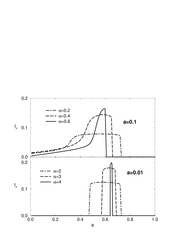
FIG. 1.: The information $I_{\alpha}$ as a function of $\theta$ without self-control for $a=0.1$ (top) and $a=0.01$ (bottom) for several values of $\alpha$.

FIG. 2.: The evolution of the overlap $m_{t}$ for several initial values $m_{0}$, with $q_{0}=0.01=a$ and $\alpha=3$ for the model with self-control (right) and the optimal threshold model (left). The dashed curves are a guide to the eye.

FIG. 3.: The basin of attraction as a function of $\alpha$ for $a=0.01$ and initial $q_{0}=a$ for the self-controlled model (full line) and the optimal threshold model (dashed line).

FIG. 4.: The information $I_{\alpha}$ as a function of $\alpha$ for the self-controlled model with several values of $a$.

FIG. 5.: The maximal information $I_{max}$ and $\alpha_{max}a|\ln(a)|$ as a function of $|\ln(a)|$.

FIG. 6.: The information $I_{\alpha}$ as a function of the loading $\alpha$ for $a=0.1$ and initial value $q_{0}=a$ with self-control and with fixed threshold $\theta_{0}$. Analytic results are compared with simulations for $N=10^{6}$ and $C=100,200$.