Role of Spatial Amplitude Fluctuations in Highly Disordered s-Wave Superconductors

The effect of strong disorder on superconductivity has been a subject of considerable interest, both theoretically [2, 3] and experimentally [4, 5], for a long time. A generally accepted physical picture of how the superconducting (SC) state is destroyed and the nature of the non-SC state has not yet emerged. Much of the theoretical work (“pairing of exact eigenstates” [2, 6] or diagrammatics [3, 7]) assumes that the pairing amplitude $\Delta({\bf r})$ is uniform in space (${\bf r}$-independent) even for a highly disordered SC; see however [8, 9]. Recent work on universal properties at the SC-insulator transition [10] has also ignored amplitude fluctuations, since phase fluctuations are presumably responsible for critical properties.

In this paper we consider a simple model of a 2D s-wave superconductor at $T=0$ in a random potential, defined by eqn. (1) below, and analyze it in detail within a Bogoliubov-deGennes (BdG) framework [11]. Our goal is to see how the local pairing amplitude $\Delta({\bf r})$ varies spatially in the presence of disorder, and the effect of this inhomogeneity on physically relevant correlation functions. Our results can be summarized as follows:

(1) With increasing disorder, the distribution $P(\Delta)$ of the local paring amplitude $\Delta({\bf r})$ becomes very broad, eventually developing considerable weight near $\Delta\approx 0$.

(2) The spectral gap in the one-particle density of states persists even at high disorder in spite of the growing number of sites with $\Delta({\bf r})\approx 0$. A detailed understanding of this surprising effect emerges from a study of the spatial variation of $\Delta({\bf r})$ and of the BdG eigenfunctions.

(3) There is substantial reduction in the superfluid stiffness and off-diagonal correlations with increasing disorder, however, the amplitude fluctuations by themselves cannot destroy the superconductivity.

(4) Phase fluctuations about the inhomogeneous BdG state are described by a quantum XY model whose parameters, compressibility and phase stiffness, are obtained from the BdG results. A simple analysis of this effective model within a self-consistent harmonic approximation leads to a transition to a non-SC state.

We conclude with some comments on the implications of our results for experiments on disordered films.

We model the 2D disordered s-wave SC by an attractive Hubbard model with on-site disorder:

$${\cal H}={\cal K}-|U|\sum_{i}n_{i\uparrow}n_{i\downarrow}+\sum_{i,\sigma}(V_{i}-\mu)n_{i\sigma}.$$ (1)

${\cal K}=-t\sum_{<ij>,\sigma}(c_{i\sigma}^{{\dagger}}c_{j\sigma}+h.c.)$ is the kinetic energy, $c_{i\sigma}^{{\dagger}}$ ($c_{i\sigma}$) the creation (destruction) operator for an electron with spin $\sigma$ on a site ${\bf r}_{i}$ of a square lattice, $t$ the near-neighbor hopping, $|U|$ the pairing interaction, $n_{i\sigma}=c_{i\sigma}^{{\dagger}}c_{i\sigma}$, and $\mu$ the chemical potential. The random potential $V_{i}$ is chosen independently at each ${\bf r}_{i}$ from a uniform distribution $[-V,V]$; $V$ thus controls the strength of the disorder.

We begin by treating the spatial fluctuations of the pairing amplitude using the standard BdG equations [11]:

$$\left(\matrix{\hat{\xi}&\hat{\Delta}\cr\hat{\Delta}^{*}&-\hat{\xi}^{*}}\right)\left(\matrix{u_{n}({\bf r}_{i})\cr v_{n}({\bf r}_{i})}\right)=E_{n}\left(\matrix{u_{n}({\bf r}_{i})\cr v_{n}({\bf r}_{i})}\right)$$ (2)

where $\hat{\xi}u_{n}(r_{i})=-t\sum_{\hat{\delta}}u_{n}({\bf r}_{i}+\hat{\delta})+(V_{i}-\tilde{\mu_{i}})u_{n}({\bf r}_{i})$ and $\hat{\Delta}u_{n}({\bf r}_{i})=\Delta({\bf r}_{i})u_{n}({\bf r}_{i})$, and similarly for $v_{n}({\bf r}_{i})$. Here $\hat{\delta}=\pm{\hat{\bf x}},\pm{\hat{\bf y}}$ and $\tilde{\mu_{i}}=\mu+|U|n_{i}/2$ incorporates the site-dependent Hartree shift in presence of disorder. Starting with an initial guess for $\Delta({\bf r}_{i})$’s and $\tilde{\mu_{i}}$ we numerically solve for the BdG eigenvalues $E_{n}$ and eigenvectors $\left(u_{n}({\bf r}_{i}),v_{n}({\bf r}_{i})\right)$ on a finite lattice of $N$ sites with periodic boundary conditions. We then calculate the local pairing amplitudes and number density at $T=0$, given by

$$\Delta({\bf r}_{i})=|U|\sum_{n}u_{n}({\bf r}_{i})v_{n}^{*}({\bf r}_{i}),~{}~{}~{}n_{i}=\sum_{n}|v_{n}({\bf r}_{i})|^{2}$$ (3)

and iterate the process until self-consistency is achieved for $n_{i}$ and $\Delta({\bf r}_{i})$ at each site. $\mu$ is determined by $1/N\sum_{i}n_{i}=\langle n\rangle$, where $\langle n\rangle$ is the average density.

We have studied the model (1) for a range of parameters: $1\leq|U|/t\leq 8$ and $0\leq V/t\leq 12$ on lattices of size $N=12\times 12$ (some checks were made on $24\times 24$ systems). We focus below on $|U|/t=2$ and $4$, $\langle n\rangle=0.875$; similar results are obtained for other parameters. The number of iterations necessary to obtain self-consistency grows with disorder; we have checked that the same solution is obtained for different initial guesses. Results are averaged over 16-20 different realizations of the disorder.

The distribution $P(\Delta)$ of local pairing amplitudes for $|U|=4$ is plotted in Fig. 1. For $V\stackrel{{{}_{<}}}{{{}_{\sim}}}0.25t$, $P(\Delta)$ has a sharp peak near the $V=0$ BCS value of $\Delta_{0}\simeq 1.36t$. In the small $V$ limit, pairing of exact eigenstates is justified, since this naturally leads [12] to uniform $\Delta({\bf r})$. However, this approximation fails with increasing $V$ as $P(\Delta)$ becomes extremely broad for $V\sim t$, eventually becoming rather skewed at $V\geq 2t$ with a large number of sites with $\Delta({\bf r})\approx 0$.

FIG. 1.: The distribution $P(\Delta)$ of the pairing amplitude $\Delta({\bf r}_{i})$ for different disorder strengths $V$. For small $V$, $P(\Delta)$ is peaked around the BCS $\Delta_{0}$, but becomes increasingly broad at higher $V$, indicative of a highly inhomogeneous state.

FIG. 2.: Density of states $N(\omega)$ for three disorder strengths $V$ which show the the persistence of a spectral gap at all disorder; (Note the different vertical scale for each case).

To study how the spectral gap evolves as the pairing amplitude becomes highly inhomogeneous, we look at the (disorder averaged) one-particle density of states (DOS) $N(\omega)=1/N\sum_{n}\delta(\omega-E_{n})$, defined in terms of the BdG eigenvalues $E_{n}$. (Numerically, $\delta$-functions are broadened into Lorentzians with a width of order spacing between $E_{n}$’s). From Fig. 2 we see that with increasing disorder the DOS pile-up at the gap edge is progressively smeared out, and that states are pushed up to higher energies. But the most remarkable feature of Fig. 2 is the presence of a finite spectral gap even at high disorder. While we can not rule out an exponentially small tail in the low energy DOS from a finite system calculation, we always found, for each disorder realization, that the lowest BdG eigenvalue remains non-zero and of the order of the zero-disorder BCS gap; see also Fig. 3(a). We also emphasize that approximate treatments of the BdG equations [13], which do not treat the local amplitude fluctuations properly, miss this remarkable feature, as do simplified models in which $\Delta({\bf r}_{i})$’s are assumed to be independent random variables at each site.

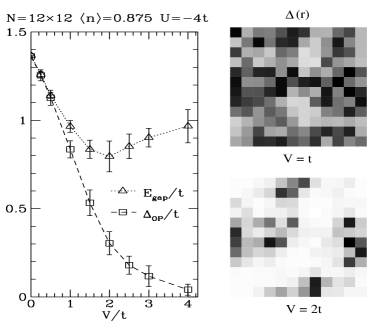
FIG. 3.: (a) Left panel: $T=0$ spectral gap $E_{\rm gap}$ and order parameter $\Delta_{\rm OP}$ (see text) as functions of disorder $V$. The two coincide for small $V$ but become very different at large disorder. (b) Right Panel: Gray-scale plot showing the spatial variation of $\Delta({\bf r}_{i})$ for the same disorder configuration with different $V$. Larger $\Delta({\bf r}_{i})$’s are indicated by darker shades. Note the spatially correlated structures at $V=2t$ with “SC islands” separated by a “sea” of nearly vanishing $\Delta$’s.

To understand the persistence of a finite spectral gap at high disorder, when a large fraction of the sites have near vanishing pairing amplitude, it is useful to study the spatial variation of of the $\Delta({\bf r}_{i})$’s and the BdG eigenvectors $\left(u_{n}({\bf r}_{i}),v_{n}({\bf r}_{i})\right)$ for individual realizations of the disorder potential. A particularly simple picture emerges at high disorder: there are spatially correlated clusters of sites at which $\Delta({\bf r}_{i})$ is large (“SC islands”), and these are separated by large regions where $\Delta({\bf r}_{i})\approx 0$ (see Fig. 3(b)). We find that the SC islands correlate well with regions where the absolute magnitude of the random potential $|V_{i}|$ is small; deep valleys and high mountains in the potential do not allow for number fluctuations and are thus not conducive to pairing. The density $n({\bf r})$ is also highly inhomogeneous, and for moderate $|U|$ ($\geq 4t$) and high disorder, we have found clear evidence for “particle-hole mixing in real space”, i.e., a spatial correlation between $\Delta({\bf r})$ and $n({\bf r})/2[1-n({\bf r})/2]$ [14].

At high disorder, we found that the eigenfunctions corresponding to low-lying excitations live entirely on the SC islands (i.e., the darker regions in Fig. 3 (b)) resulting in the finite spectral gap. On the other hand, regions where the pairing amplitude is small correspond to very large values of $|V_{i}|$, as explained above, and thus support even higher energy excitations. Clearly this simple picture of SC islands is well defined only in the large disorder regime, nevertheless, it is useful for understanding the spectral gap in this limit. In the opposite limit of low disorder, of course, the BCS-like spectral gap is obvious.

We next turn to the question of how superconductivity is affected in the highly inhomogeneous BdG state. The off-diagonal long range order parameter $\Delta_{\rm OP}$ is defined by the (disorder averaged) correlation function $\langle c_{i\uparrow}^{{\dagger}}c_{i\downarrow}^{{\dagger}}c_{j\downarrow}c_{j\uparrow}\rangle\rightarrow\Delta_{\rm OP}^{2}/|U|^{2}$ for large $|{\bf r}_{i}-{\bf r}_{j}|$. From Fig. 3 (a) we see that $\Delta_{\rm OP}$ is the same as the spectral gap (and both equal the uniform pairing amplitude) for small disorder, as expected from BCS theory. However beyond a certain $V$ the two quantities deviate from each other: in contrast to the spectral gap, the order parameter decreases with increasing disorder; (we find that $\Delta_{\rm OP}\simeq\int d\Delta\Delta P(\Delta)$, i.e., the average value of the pairing amplitude).

The superfluid stiffness $D_{s}^{0}$ is given by[15] $D_{s}^{0}/\pi=\langle-k_{x}\rangle-\Lambda_{xx}(q_{x}=0,q_{y}\rightarrow 0,\omega=0)$. The diamagnetic term $\langle-k_{x}\rangle$, is one-half (in 2D) the kinetic energy $\langle-{\cal K}\rangle$, and the paramagnetic term $\Lambda_{xx}$ is the (disorder averaged) transverse current-current correlation function. We have also checked that the charge stiffness $D^{0}$ is equal to $D_{s}^{0}$. ($D^{0}$ is the strength of the delta-function in $\sigma(\omega)$, and given in terms of $\Lambda_{xx}({\bf q}=0,\omega\rightarrow 0)$ [15]).

FIG. 4.: The $T=0$ BdG superfluid stiffness $D_{s}^{0}$ and the spectral gap $E_{\rm gap}$ plotted as a function of disorder strength for two different values of attraction $|U|$. Note that irrespective of whether $D_{s}^{0}$ is larger than or comparable to $E_{\rm gap}$ at $V=0$, the gap persists with increasing disorder while stiffness decreases.

The $D_{s}^{0}$ calculated within BdG theory shows a large reduction [16] by two orders of magnitude with increasing disorder; see Fig. 4. We see that for $U=-2t$, at $V=0$, $D_{s}^{0}\gg E_{\rm gap}$, characteristic of weak coupling BCS theory, where the vanishing of the gap determines $T_{c}$, while for $U=-4t$, $D_{s}^{0}$ and $E_{\rm gap}$ are comparable at $V=0$, indicative of an intermediate coupling regime [17] where thermal phase fluctuations are important for determining $T_{c}$ [18]. However, for all $|U|/t$, we always find $D_{s}^{0}\ll E_{\rm gap}$ at large disorder, and thus phase fluctuations have to be taken into account. In fact the reason why $D_{s}^{0}$ is not driven to zero at large $V$ within the BdG framework is due to the neglect of these fluctuations.

To make a rough estimate of the effect of phase fluctuations about the inhomogeneous BdG state we use a quantum XY model with an effective Hamiltonian [2] $H_{\theta}=-(\kappa/8)\sum_{j}\dot{\theta}_{j}^{2}+(D_{s}^{0}/4)\sum_{\langle jk\rangle}\cos(\theta_{j}-\theta_{k})$, whose parameters are obtained from the preceding analysis: the bare $D_{s}^{0}$ is the BdG superfluid stiffness and $\kappa=dn/d\mu$ is the BdG compressibility. The large reduction in $dn/d\mu$ with disorder seen in Fig. 5 (a) can be understood qualitatively at large $V$ in terms of the charging energy of the SC islands. Note that, in this simplified description using $H_{\theta}$, we ignore the inhomogeneity in the local bare stiffness and charging energies.

FIG. 5.: (a) Left Panel: The compressibility $dn/d\mu$ as a function of disorder $V$. (b) Right Panel: The superfluid density $D_{s}/\pi$ as a function of disorder $V$. By including phase fluctuation a transition is obtained at $V_{c}$ which is very close to that predicted by QMC [21].

We use a variational approximation [19] to estimate the renormalized superfluid stiffness $D_{s}=D_{s}(\kappa,D_{s}^{0})$, by finding the best harmonic $H_{\rm trial}=-(\kappa/8)\sum_{j}\dot{\theta}_{j}^{2}+(D_{s}/8)\sum_{\langle jk\rangle}(\theta_{j}-\theta_{k})^{2}$, which describes $H_{\theta}$. The phase variables $\theta_{i}$ are assumed to live on a lattice with lattice constant set by the BdG coherence length $\xi_{0}$. For $U=-4t$ we choose $\xi_{0}\simeq 1.8$ [20] by demanding that the renormalized $D_{s}$ at $V=0$ agrees with that obtained from quantum Monte Carlo (QMC) [21] ($D_{s}/\pi\simeq 0.45t$) for the pure case.

We now calculate the renormalized $D_{s}$ as a function of disorder, using the $V$-dependent $\kappa$ and $D_{s}^{0}$ from the BdG analysis as input and keeping $\xi_{0}$ fixed; (details will be presented elsewhere [14]). As shown in Fig. 5 (b), $D_{s}$ is driven to zero beyond a critical disorder $V_{c}$ which is in very reasonable agreement with QMC [21]. Thus a transition to a non-SC (insulating) state is indeed obtained by incorporating the effects of phase fluctuations about the inhomogeneous BdG state.

We emphasize that the finite spectral gap obtained in the BdG analysis at large $V$ will survive inclusion of phase fluctuations, since this gap is related to the inhomogeneous SC islands. A key question is whether the inhomogeneous $\Delta({\bf r})$ leading to a spectral gap in the insulating state persists all the way down to $|U|/t\ll 1$. A definitive answer cannot be obtained since weak coupling BdG calculations are plagued by severe finite size effects [22]. It is important to note that the gap persists in the $|U|=2t$ case (see Fig. 4(a)) which in the $V=0$ limit has $D_{s}^{0}\gg E_{\rm gap}$, characteristic of weak coupling SC. The available numerical results suggest that even for weak coupling, $\Delta({\bf r})$ inhomogeneities are generated on the scale of the coherence length, which eventually show up as SC islands at large disorder. This would suggest persistence of the gap. In contrast, some tunneling experiments [5](c) show a finite DOS N(0) with increasing disorder, which then points to physical effects beyond those in the simplest model studied here. One possibility is that Coulomb interactions in the presence of disorder lead to an effective $|U|$ which is ${\bf r}$-dependent, and regions with $|U_{i}|\approx 0$ lead to finite $N(0)$. Another possibility is that Coulomb interactions plus disorder lead to the formation of local moments which are pair breaking.

Another implication of our results for experiments is that SC-Insulator transitions in disordered films are often described in terms of two different paradigms: homogeneously disordered films (driven insulating by the vanishing of the gap) and granular films (driven by vanishing of the phase stiffness). In our simple model, although the system was homogeneously disordered at the microscopic level, granular SC-like structures developed in so far as the pairing amplitude was concerned. It would be very interesting to use STM measurements to study variations in the local density states to shed more light on this question.

Acknowledgements: We would like to thank A. Paramekanti, T. V. Ramakrishnan and R. T. Scalettar for useful discussions.

REFERENCES

- [1]
- [2] T. V. Ramakrishnan, Physica Scripta, T27, 24 (1989).
- [3] D. Belitz and T. Kirkpatrick, Rev. Mod. Phys., 66, 261 (1994); M. Sadovskii, Phys. Rept., 282, 225 (1997).
- [4] A. Hebard, in “Strongly Correlated Electronic Systems”, edited by K. Bedell et al., (Addison-Wesley, 1994).
- [5] (a) D.B. Haviland, Y.Liu, and A.M. Goldman, Phys. Rev. Lett. 62 2180, (1989); (b) A.E. White, R.C. Dynes, and J.P. Garno, Phys. Rev. B33, 3549 (1986); (c) J.M. Valles, R.C. Dynes, and J.P. Garno, Phys. Rev. Lett. 69, 3567 (1992).
- [6] M. Ma and P. A. Lee, Phys. Rev. B32,5658 (1985); G. Kotliar and A. Kapitulnik, Phys. Rev. B33, 3146 (1986).
- [7] R.A. Smith and V. Ambegaokar, Phys. Rev. B45, 2463 (1992); R.A. Smith, M. Reizer and J. Wilkins, Phys. Rev. B51, 6470 (1995).
- [8] L.N. Bulaevskii, S.V. Panyukov, and M.V. Sadovskii, Sov. Phys. JETP 65, 380 (1987).
- [9] M. Franz et al., Phys. Rev. B56, 7882 (1997).
- [10] M. P. A. Fisher, G. Grinstein and S. M. Girvin, Phys. Rev. Lett. 64, 587 (1990).
- [11] P. G. de Gennes, Superconductivity in Metals and Alloys (Benjamin, New York, 1966).
- [12] In this approximation and are proportional to the exact eigenstates of the non-interacting disordered Hamiltonian. This, together with the assumption of an -independent local DOS, leads to a uniform [11]. We have found that the local DOS becomes highly nonuniform even for moderate disorder.
- [13] For instance, T. Xiang and J. M. Wheatley, Phys. Rev. B51, 11721 (1995), imposed self-consistency on the average of over all sites. This washed out the amplitude fluctuations and led, incorrectly, to a spectral gap which closes with increasing disorder.
- [14] A. Ghosal, M. Randeria and N. Trivedi, (unpublished).
- [15] D.J. Scalapino, S.R. White, and S.C. Zhang, Phys. Rev. B47, 7995 (1993).
- [16] An inhomogeneous state will neccessarily have a small superfluid stiffness; see, e.g., A. Paramekanti, N. Trivedi and M. Randeria, Phys. Rev. B57, 11639 (1998)
- [17] M. Randeria, N. Trivedi, A. Moreo, and R. Scalettar, Phys. Rev. Lett. 69, 2001 (1992); N. Trivedi and M. Randeria, Phys. Rev. Lett. 75, 312 (1995).
- [18] V. Emery and S. Kivelson, Nature 374, 434 (1995).
- [19] D. Wood and D. Stroud, Phys. Rev. B25, 1600 (1982); S. Chakravarty et al., Phys. Rev. Lett. 56, 2303 (1986).
- [20] The renormalized is highly sensitive to the choice of . ( e.g., in weak coupling BCS theory with , one has ). Our choice of , by comparing with QMC, is also consistent with independent estimates from the BdG analysis.
- [21] N. Trivedi, R. T. Scalettar, and M. Randeria, Phys. Rev. B54, R3756 (1996). The convention used in this paper is such that our .
- [22] From QMC studies of model (1), C. Huscroft and R. T. Scalettar, (cond-mat/9804122) have claimed that the gap vanishes for using maximum entropy techniques. We believe that their results are at a high temperature, given the gap scale, to warrant this conclusion.