Spatially-resolved studies of chemical composition,
critical temperature, and critical current density of
a YBa₂Cu₃O_7-δ thin film

Abstract

Spatially-resolved studies of a YBa₂Cu₃O_7-δ thin film bridge using electron probe microanalysis (EPMA), low-temperature scanning electron microscopy (LTSEM), and magneto-optical flux visualization (MO) have been carried out. Variations in chemical composition along the bridge were measured by EPMA with 3 $\mu$m resolution. Using LTSEM the spatial distributions of the critical temperature, $T_{c}$, and of the local transition width, $\Delta T_{c}$, were determined with 5 $\mu$m resolution. Distributions of magnetic flux over the bridge in an applied magnetic field have been measured at 15 and 50 K by magneto-optical technique. The critical current density $j_{c}$ as a function of coordinate along the bridge was extracted from the measured distributions by a new specially developed method. Significant correlations between $j_{c}$, $T_{c}$, $\Delta T_{c}$ and cation composition have been revealed. It is shown that in low magnetic fields deviation from the stoichiometric composition leads to a decrease in both $T_{c}$ and $j_{c}$. The profile of $j_{c}$ follows the $T_{c}$-profile on large length scales and has an additional fine structure on short scales. The profile of $j_{c}$ along the bridge normalized to its value at any point is almost independent of temperature.

I Introduction

The complicated crystal structure of high-$T_{c}$ superconductors (HTSC) leads to their substantial spatial inhomogeneity which is specially important because of the very short coherence length in those materials. Consequently, spatially-resolved studies of HTSC are very effective both to evaluate the general quality of the samples and to determine local values of important parameters. The quantities measured in the experiments which do not allow spatial resolution are averaged over rather broad distributions. Moreover, in some cases the properties of the whole sample can be determined by one or few “bottlenecks”. This appears to be one of the main obstacles to adequate interpretation of experimental data and optimization of the performance of superconductor devices.

Only a combination of different spatially-resolved methods allows one to relate different physical properties of the material in order to facilitate the development of reliable theoretical models. As examples of such combinations several works can be mentioned. In Ref. [1], spatially-resolved X-ray analysis together with measurements of voltage flicker noise allowed the study of the relation between the noise level and a distribution of microstrains, in order to work out a relevant theoretical model. Analysis of the correlation between locally measured cation composition, critical temperature, and flicker noise allowed the development of a theoretical model for cation defect formation in YBa₂Cu₃O₇ films[2].

Spatial distribution of the critical current density, $j_{c}$, is also of great interest. It is a quantity that is important for both HTSC applications and understanding the pinning mechanisms. Distribution of $j_{c}$ can be inferred from the distributions of magnetic field measured, e.g. by magneto-optical (MO) imaging. Unfortunately, most MO studies are restricted to a qualitative analysis of magnetic field distributions since they are quite complicated even for a homogeneous superconductor (see Ref. [3] and references therein for a review). Only few works[4, 5] have been devoted to analyzing the distributions of current density, $j$, restored from MO images. The results give evidence of an extremely inhomogeneous $j$-distributions and facilitate revealing factors limiting current density. Extensive efforts in this direction seem to be crucially important for subsequent progress in creation of high-$j_{c}$ HTSC structures.[6]

In this work we present a quantitative study of $j_{c}$-inhomogeneity along a HTSC bridge using the MO technique. By means of low temperature scanning electron microscopy (LTSEM), the spatial distribution of the critical temperature, $T_{c}$, has been measured for the same bridge. Simultaneous use of MO and LTSEM has earlier proved to be successful for predicting the locations in a thin film bridge where burn-out is caused by a large transport current[7]. The present paper reports the results of a comprehensive quantitative investigation of the correlation between the spatial distributions of $j_{c}$, $T_{c}$ and chemical composition.

II Experimental

A Sample preparation

Films of YBa₂Cu₃O_7-δ were grown by dc magnetron sputtering [8] on LaAlO₃ substrate. X-ray analysis and Raman spectroscopy confirmed that the films were $c$-axis oriented and had a high structural perfection. Several samples, shaped as a bridge, were formed by a standard lithography procedure. One of them, with dimensions $460\times 110\times 0.2$ $\mu$m³, was used for the present studies. The absence of pronounced weak links, and other defects which reduce the total critical current $I_{c}$, was confirmed by means of LTSEM[9], and MO imaging. The critical current density, $j_{c}$, determined by transport measurements was larger than $10^{5}$ A/cm² at 77 K. The critical temperature defined by the peak of the temperature derivative of resistance $dR/dT$ was $T_{c}=92.2$ K. The transition width defined by the width of $dR/dT$ peak was $\Delta T_{c}=2.2$ K.

B Quantitative electron probe microanalysis

Spatially-resolved measurements of chemical composition and film thickness have been performed using electron probe microanalysis on an X-ray spectral microanalyzer Camebax[2]. The electron energy in the exciting beam was 15 keV which allowed us to register simultaneously the spectral lines Y L$\alpha$, Ba L$\alpha$, Cu K$\alpha$, and O K$\alpha$ for all the elements, and determine the film thickness in the same experiment. The absolute accuracy of the chemical composition determination is 0.3, 1.0, 1.2, and 2.0% for Y, Ba, Cu and O, respectively. Such accuracy has been achieved by a special computer program to calculate the distribution of X-ray emission from both thin film and substrate under irradiation by the electron beam (see Ref. [2] for details). The spatially-varying part of the composition is determined with three times better accuracy for all the elements due to improving the measurement procedure as follows: (i) we use computerized control of the probe current while accumulating 10⁵ pulses from the X-ray detector, (ii) a special computer program enabling composition determination at 150 points of the film during one experimental run was implemented, and (iii) we performed a running calibration based on comparison of the line intensities with those of a pure YBa₂Cu₃O_7-δ single crystal placed in the same chamber. The spatial resolution of the method is 3 $\mu$m.

C Low-temperature scanning electron microscopy

The LTSEM technique originally developed to study conventional superconductors[10, 9] has recently been adapted for determination of spatial distributions of critical temperature, or $T_{c}$-maps[11, 12]. The method is based on monitoring the local transition into the normal state due to heating by a focused electron beam. Heating by the beam elevates the temperature locally causing a change in the local resistivity. As a result, a change in the voltage occurs across the sample biased by a transport current. Since the electron beam induced voltage (EBIV) is proportional to the temperature derivative of the local resistivity, the signal reaches its maximum at the temperature equal to the local value of $T_{c}$. The width of the maximum corresponds to the local transition width, $\Delta T_{c}$. Scanning the electron beam over the film allows us to determine the spatial distribution of both $T_{c}$ and $\Delta T_{c}$. The spatial resolution for $T_{c}$ and $\Delta T_{c}$ determination can be improved by a proper treatment of the EBIV distributions taking into account heat diffusion from the irradiated region into surrounding areas. As a result, a spatial resolution up to 2 $\mu$m and a temperature resolution up to 0.2 K can be achieved[11, 12].

The LTSEM measurements were carried out with an automated scanning electron microscope CamScan Series 4-88 DV100 equipped with a cooling system ITC4 and a low-noise amplifier for voltage signals. The temperature could be maintained to within 0.1 K in the range 77-300 K. The bias current $I$ was varied from 0.2 to 2.0 mA so that the value of $I$ was large enough to detect EBIV and small enough to avoid distortion of the transition by bias current. EBIV was measured using a simple four-probe scheme. To extract the local EBIV signal, lock-in detection was used with a beam-modulation frequency of 1 kHz. The electron beam current was 10^-8 A while the acceleration voltage was 10 kV.

D Magneto-optical technique

Our system for flux visualization is based on the Faraday rotation of a polarized light beam illuminating an MO-active indicator film placed directly on top of the sample surface. The rotation angle grows with the magnitude of the local magnetic field perpendicular to the HTSC film, and by using crossed polarizers in an optical microscope one can directly visualize and quantify the field distribution across the sample area. As Faraday-active indicator we use a Bi-doped yttrium iron garnet film with in-plane anisotropy[13]. The indicator film was deposited to a thickness of 5 $\mu$m by liquid phase epitaxy on a gadolinium gallium garnet substrate. Finally, a thin layer of aluminum was evaporated onto the film in order to reflect the incident light and thus providing a double Faraday rotation of the light beam. The images were recorded with an eight-bit Kodak DCS 420 CCD camera and transferred to a computer for processing. After each series of measurements at a given temperature, the temperature was increased above $T_{c}$ and an in-situ calibration of the indicator film was carried out. As a result, possible errors caused by inhomogeneities of both indicator film and light intensity were excluded. The experimental procedure is described in more detail in Ref. [14].

III Results

To report the experimental results we employ the following notations. The $x$-axis is directed across the bridge, the edges being located at $x=\pm w$, the $y$-axis points along the bridge, and the $z$-axis is normal to the film plane. In what follows, the distributions of the chemical compositions, $T_{c}$, $\Delta T_{c}$ and $j_{c}$ are analyzed as functions of $y$.

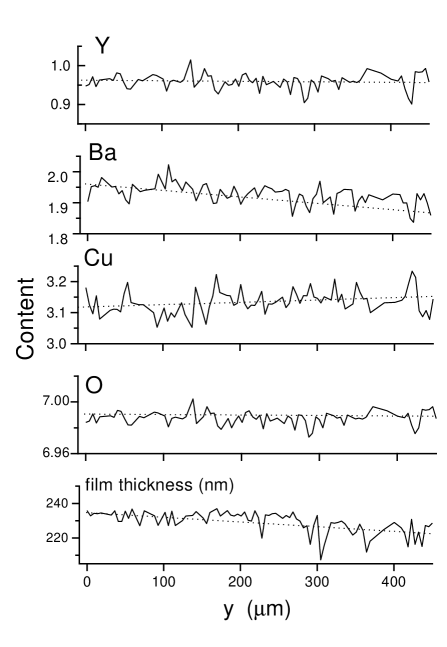
FIG. 1.: Variations in microscopic chemical composition along YBa₂Cu₃O_7-δ bridge and variations in film thickness measured by EPMA. Dotted lines show linear fits to data. A gradient in Ba and Cu content is clearly seen.

A Chemical composition variation

Variations in Y, Ba, Cu, and O contents along the YBa₂Cu₃O_7-δ bridge are shown in Fig. 1. A systematic gradients in Ba and Cu content are clearly visible and indicated by the dotted lines representing linear fits to the data. Note, that the left part of the bridge (small $y$) is closer to the stoichiometric composition, YBa₂Cu₃O₇, than the right part. It can also be seen from Fig. 1 that, in contrast to the cations, the oxygen is distributed rather uniformly over the bridge. A uniform oxygen distribution in YBa₂Cu₃O_7-δ films has been observed also earlier[1, 2]. It is probably a consequence of high diffusion coefficient of oxygen in the YBa₂Cu₃O_7-δ lattice. Thus, we can focus on variations in the cation composition only. The composition diagram for Y_yBa_1-x-yCu_xO_z in the vicinity of stoichiometric YBa₂Cu₃O₇ composition projected on the plane $z=0$ is shown in Fig. 2. The open (solid) data points correspond to local compositions measured in the left (right) part of the bridge.

Except the long-scale gradient in Ba and Cu, short-scale oscillations in the cation composition can be seen from Fig. 1. A careful analysis of the data shows that short-scale oscillations in Y and Ba content are correlated with each other and anti-correlated with those in Cu content. As a result, the experimental data points in Fig. 2 are mainly spread along the direction towards CuO oxide. To clarify the origin of this phenomenon

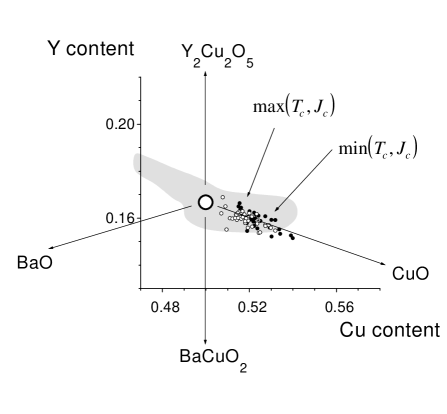
FIG. 2.: Composition diagram of Y_yBa_1-x-yCu_xO_z in the vicinity of stoichiometric YBa₂Cu₃O₇ composition projected on the plane $z=0$. The stoichiometric composition is shown by the large open circle. Small open (solid) circles correspond to local compositions measured in the left (right) part of the bridge. The lines show directions towards known stable compounds. Gray area shows the region[2] where superconducting properties of the material are only weakly sensitive to the composition. The closer local composition to the stoichiometric one, the higher local values of $T_{c}$ and $J_{c}$.

we carried out SEM studies of the bridge surface which revealed the presence of submicron CuO inclusions. Inclusions are formed due to excess of Cu in YBa₂Cu₃O₇ lattice and lead to a slightly nonuniform distribution of Cu on micron scale. Note that these short-scale variations in cation composition have nothing to do with the long-scale gradient in Ba and Cu content. In this work we are interested in the long-scale composition variations only. Below they will be compared to the long-scale variations in $T_{c}$ and $j_{c}$.

B $T_{c}$ and $\Delta T_{c}$-profiles

The EBIV profiles along the bridge for four temperatures are presented in Fig. 3. Each point is obtained by averaging local EBIV along the $x$-direction, i.e., over the bridge cross-section. A systematic inhomogeneity of the bridge can be seen. Large EBIV for higher temperatures in the left part of the bridge corresponds to higher $T_{c}$ there, while in the right part, EBIV is large at low temperatures indicating lower $T_{c}$.

The spatial distributions of the critical temperature $T_{c}$ and the transition width, $\Delta T_{c}$, with 5 $\mu$m resolution has been determined according to the procedure mentioned in Sec. II C and described in more detail in Ref.[11] and [12]. The profiles $T_{c}(y)$ and $\Delta T_{c}(y)$, as shown in Fig. 4, have been calculated by averaging over 20 points across the bridge. The standard deviation is less than the actual accuracy of the $T_{c}$ and $\Delta T_{c}$ determinations which is $0.2$ K. One can clearly see a gradient in $T_{c}$ which is especially large in the right part of the bridge. Note that a decrease in $T_{c}$ is accompanied by an increase in $\Delta T_{c}$. Larger transition width, $\Delta T_{c}$, in the right part of the bridge is most probably related to an inhomogeneous distribution of $T_{c}$ on the scales shorter than LTSEM resolution, 5 $\mu$m. Such a short-scale $T_{c}$-inhomogeneity can hardly be expected in the left part of the bridge where $T_{c}$ approaches its maximal value, $\geq 93$ K, corresponding

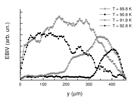
FIG. 3.: Profiles of the EBIV measured by LTSEM along the YBa₂Cu₃O_7-δ bridge for different temperatures. Essential spatial inhomogeneity of EBIV is clearly seen.

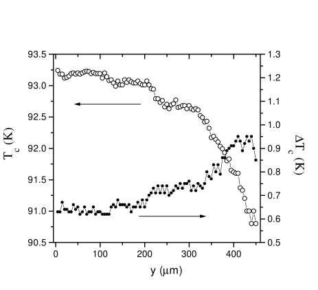
FIG. 4.: Profiles of the critical temperature, $T_{c}$, and of the transition width, $\Delta T_{c}$, along the bridge determined from LTSEM data.

to a stoichiometric composition of the material.

It should be noted that only the values of $T_{c}$ greater than some minimum temperature, $T_{\min}\approx 90.7$ K, can be determined by the present method. We believe that the temperature $T_{\min}$ corresponds to formation of superconducting percolation cluster, and at $T<T_{\min}$ the EBIV falls below our experimental resolution. The results presented in Fig. 4 are obtained by averaging over the regions with $T_{c}>T_{\min}$ corresponding to 66% of the area for our sample. The value $p_{c}=66\%$ for the percolation threshold seems reasonable since for an infinite random two-dimensional system $p_{c}\approx 50\%$ and the bridge shape seems intermediate between a 2D and a 1D geometry.

C MO results: $j_{c}$-profiles

The magnetic field distributions in perpendicular applied fields up to 35 mT have been measured using the MO technique at $T=15$ K and 50 K. A typical MO image of the narrow strip part of the bridge is shown in Fig. 5. Figure 6 shows a typical profile of the absolute value of the $z$-component of magnetic induction across the bridge for an external field $B_{a}=21$ mT. The profile is obtained by averaging the flux distribution over a 110 $\mu$m length along the bridge.

The data were fitted to the Bean model for thin strip geometry[15, 16]. For the indicator film placed at the height $h$ above the bridge the $z$-component of magnetic induction is given by the expression [14],

$$B(x) = \frac{B_{c}}{4}\left\{\ln\frac{\left[(x+a)^{2}+h^{2}\right]\left[(x-a)^{2}+h^{2}\right]}{\left[(x+w)^{2}+h^{2}\right]\left[(x-w)^{2}+h^{2}\right]}-\frac{4}{\pi}\int^{a}_{-a}\frac{x^{\prime}-x}{(x^{\prime}-x)^{2}+h^{2}}\arctan\left(\frac{x^{\prime}}{w}\sqrt{\frac{w^{2}-a^{2}}{a^{2}-x^{\prime 2}}}\right)dx^{\prime}\right\}+B_{a}.$$ (1)

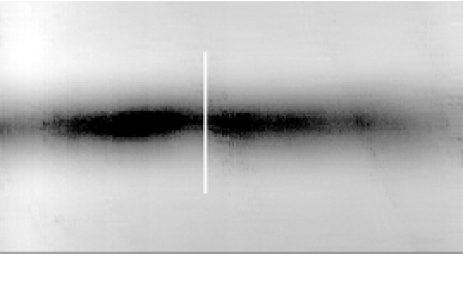
FIG. 5.: Magneto-optical image of flux distribution in a bridge in a perpendicular external field of $B_{a}=21$ mT at temperature $T=15$ K. Dark regions correspond to low flux density. In the right part of the bridge the width of the dark region is reduced indicating deeper flux penetration and, hence, lower critical current density. A region of deep flux penetration in the center of the bridge is marked by a white line.

Here

$$a=w/\cosh\left(B_{a}/B_{c}\right),\quad\quad B_{c}\equiv\frac{\mu_{0}J_{c}}{\pi}\,.$$ (2)

The quantity $a$ limits the area of field penetration (the region $|x|<a$ is vortex free). The sheet critical current density, $J_{c}$ is defined as $J_{c}=\int^{d}_{0}j_{c}(z)\,dz$, where $d$ is the film thickness.

The contact pads which are necessary for the LTSEM measurements screen the applied field to some extent. As a result, the actual external field $B_{a}$ acting upon the bridge is unknown. Therefore, Eq. (1) contains three unknown quantities, $B_{c}$, $h$, and $B_{a}$. Fortunately, the situation appears rather simple when $B_{a}\gg B_{c}$, as $a$ then becomes negligible. For $B_{a}>3B_{c}$ substituting $a=0$ into Eq. (1) leads to $\leq 1\%$ error in $B(x)$ for any $x$. The quantity $B_{a}$ then enters Eq. (1) as an additive constant, and we eliminate it by considering the difference $\delta B(x)\equiv B(x+\Delta)-B(x-\Delta)$. Here $\Delta$ is a constant shift which we chose to be equal $10\ \mu$m. The expression for $\delta B(x)$ has the form $\delta B(x)=B_{c}{\cal L}(x,h)$ with

$${\cal L}(x,h)=\frac{1}{4}\,\ln\frac{\left[(x+\Delta)^{2}+h^{2}\right]^{2}\left[(x-\Delta+w)^{2}+h^{2}\right]\left[(x-\Delta-w)^{2}+h^{2}\right]}{\left[(x-\Delta)^{2}+h^{2}\right]^{2}\left[(x+\Delta+w)^{2}+h^{2}\right]\left[(x+\Delta-w)^{2}+h^{2}\right]}$$ (3)

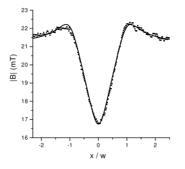
FIG. 6.: A typical magnetic field profile across the bridge averaged over distance $2w$ along the bridge. The external field was $B_{a}=21$ mT. The line shows a fit by the Bean model, Eq. (1) using $j_{c}=4.7\cdot 10^{6}$ A/cm², and $h=0.33w$.

Thus, we are left with two unknown parameters, $B_{c}$ and $h$. The experimental curves for $\delta B(x)$ were fitted by the formula (3), the parameters $B_{c}$ and $h$ being determined by minimizing the quantity

$$S=\int_{-2w}^{2w}dx\,\left[B_{c}{\cal L}(x,h)-\delta B_{\text{exp}}(x)\right]^{2}\,.$$

The condition $\partial S/\partial B_{c}=0$ implies that the two unknown parameters are related by the expression

$$B_{c}=\int_{-2w}^{2w}dx\,\delta B_{\text{exp}}(x)\,{\cal L}(x,h)\,\left[\int_{-2w}^{2w}dx\,{\cal L}^{2}(x,h)\right]^{-1}.$$ (4)

From the fitting, the height $h$ was found to be a linear function of the co-ordinate $y$,

$$h=14\,\mu\text{m}+0.006\,y\,.$$ (5)

This corresponds to a tilt angle of $\approx 0.3^{\circ}$ for the indicator film with respect to the surface of the sample.

The fitting procedure identifies good agreement between experimental and theoretical flux profiles. Figure 6 shows an example of such a fit, which also verifies the adequacy of the Bean model for our experimental situation. Applying higher external field we checked that this method, based on assumption of a $B$-independent $J_{c}$, works with a proper accuracy up to $B_{a}\approx 30$ mT. The method is therefore applied to determine $J_{c}$ values in different cross-sections of the bridge.

It should be noted that the basic expression, Eq. (1), is derived for a homogeneous infinite strip[16, 15]. Consequently, it is valid only for a smooth inhomogeneity along the bridge. One can expect that the characteristic scale of inhomogeneities which can be analyzed using Eq. (3) should be larger than the bridge width, $2w$. To estimate the accuracy of the employed method we have compared the magnetic field $B(x,\infty)$ in an infinite strip and the field $B(x,L)$ in the middle of a finite-length bridge $(-L\leq y\leq L)$. For the case of full penetration, $J=J_{c}(x/|x|)$, the difference between the fields at height $h$ is given by the expression

$$B(x,L)-B(x,\infty)=\frac{\mu_{0}J_{c}}{4\pi}\ln\frac{\left[\sqrt{(x+w)^{2}+h^{2}+L^{2}}+L\right]\left[\sqrt{(x-w)^{2}+h^{2}+L^{2}}+L\right]}{(\sqrt{x^{2}+h^{2}+L^{2}}+L)^{2}}\,.$$ (6)

This expression reaches the maximum in the bridge center, $x=0$. Substituting $h=0.33w$ and $L=w$ we find that $B(0,w)-B(0,\infty)\approx 0.15B(0,\infty)$, i. e. the field for the strip with the length $2w$ is $\approx 85\%$ of that for the infinite strip. Further, substitution of $B(x,w)$ into Eqs. (3) and (4), leads to the error about 9% in the value of restored sheet current density $J_{c}$. Thus, the proposed method allows determination of variations in $J_{c}$ on length scales 2$w$ with accuracy better than 9%.

Based on the above estimates we have averaged the experimental profiles $B(x)$ over the intervals $(y-w,y+w)$

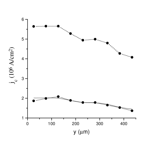
FIG. 7.: Profiles of the critical current density $j_{c}$ along the bridge measured at 15 K (upper curve) and 50 K (lower curve). Values of $j_{c}$ were calculated from the measured magnetic field distribution in external field $B_{a}=21$ mT. Solid line corresponds to $j_{c}(15\,$K$)/2.8$.

for several $y$ and then calculated the critical current density $j_{c}(y)=J_{c}(y)/d$ from Eqs. (4) and (2). The results for $T=15$ K and $T=50$ K are shown in Fig. 7. These results are obtained from $B(x)$-profiles at $B_{a}=21$ mT which we consider as an optimal value of external field. Indeed, at low applied fields $B_{a}$ our assumption $a=0$ is not valid, while at high $B_{a}$, $j_{c}(B)$-dependence becomes noticeable and the Bean model is not applicable. As seen from Fig. 7, $j_{c}$ is essentially inhomogeneous. Values of $j_{c}$ at opposite edges of the bridge differ by almost a factor of two. Since the apparent value of the critical current density can be affected by variation of the film thickness $d$, we also measured the profile of $d$ along the bridge using the EPMA technique. It can be seen from the lower panel of Fig. 1 that the variation in $d$ is about 5%. Therefore, it cannot be responsible for the observed variation in $j_{c}$ since the latter is substantially larger.

Note that the curves for $T=15$ K and $T=50$ K differ practically by a constant factor $\approx 2.8$. To illustrate this fact we show profile of the critical current for 15 K divided by 2.8 by solid line in Fig. 7.

IV Discussion

The main results of this work is the observation of a substantial sensitivity of both the critical parameters of the superconductor, $T_{c}$ and $j_{c}$, to the material composition. As the composition deviates from the stoichiometric one towards excess of Cu and Ba deficiency, both $T_{c}$ and $j_{c}$ decrease. Furthermore, although the composition varies gradually over the whole bridge, the critical parameters vary gradually in some region where the deviation from the stoichiometric composition is small, while outside this region they decrease drastically (see Figs. 1, 4 and 7). Such behavior is consistent with existence of the region in vicinity of stoichiometric composition, YBa₂Cu₃O₇, where superconducting properties are only weakly sensitive to the composition. When composition falls beyond this region, the material contains defects which dramatically affect the electronic properties and in this way reduce significantly both $T_{c}$ and $j_{c}$. Some ideas regarding the shape of this region in YBa₂Cu₃O_7-δ can be inferred from the studies of cation defect formation performed in Ref. [2]. An excess of Cu along with a Ba deficiency leads to substitution defects which neither produce substantial strain in the lattice, nor cause charge redistribution. Therefore the width of the region is rather wide in the mentioned direction, that is illustrated by Fig. 2. Change of Ba content from 1.95 to 1.85 is accompanied by only a 2 K decrease in $T_{c}$.

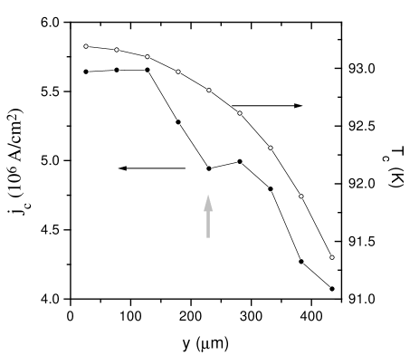
FIG. 8.: Profiles of the critical current density, $j_{c}$, at $T=15$ K, and of the critical temperature, $T_{c}$, along the bridge. Arrow marks the region of reduced $j_{c}$ which is also seen in Fig. 5 and marked by the white line.

A clear correlation between $j_{c}$ and $T_{c}$ is illustrated by Figs. 8 and 9. Despite of qualitative similarity of the $j_{c}(y)$ and $T_{c}(y)$ dependences, the critical current varies much more strongly; the variation in $T_{c}$ is $\approx 2\%$ while $j_{c}$ varies by almost a factor of two. To describe the correlation between $j_{c}$ and $T_{c}$ in a quantitative way let us note that $j_{c}(y)$ profiles for 15 and 50 K differ only by a numerical factor (see Fig. 7). Thus the critical current at large enough scale can be described as $j_{c}(T,y))=F(T)j_{c0}[T_{c}(y)]$, where $F(T)$ is a function of the temperature. It follows from Fig. 7 that $F(15\,\text{K})/F(50\,\text{K})=2.8$. In Fig. 9 the dimensionless quantity $(1-j_{c}/j_{c\,\max})$ is plotted versus the quantity $(1-T_{c}/T_{c\,\max})$ for $T=15$ and 50 K. Here $j_{c\,\max}$ and $T_{c\,\max}$ are the maximum values of $j_{c}$ and $T_{c}$ over the bridge. The data can be approximated by a power law function with the exponent $\nu\approx 0.7$. Thus, one can express the $j_{c}-T_{c}$ correlation as

$$1-J_{c}(T)/J_{c\,\max}(T)\propto(1-T_{c}/T_{c\,\max})^{\nu}\,,$$ (7)

with a temperature independent coefficient.

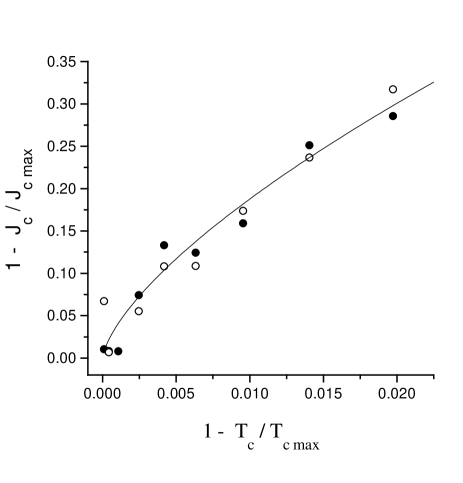
FIG. 9.: Correlation between the normalized critical current density, $J_{c}$, and critical temperature. $J_{c\,\max}$ and $T_{c\,\max}$ are the maximal values of $J_{c}$ and $T_{c}$ over the bridge. Open circles correspond to $T=50$ K while the solid ones correspond to $T=15$ K. Solid line shows the power law fit with the exponent $\nu=0.7$.

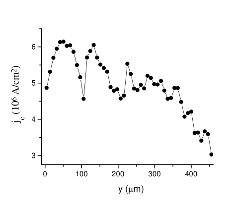
FIG. 10.: Profile of the critical current density $j_{c}$ along the bridge. The method used for determination of $j_{c}$ provides accurate results on length scales $\geq 110\mu$m. Thus, the figure illustrates the existence of $j_{c}$-inhomogeneity on short scales, but does not give a quantitative information about this short-scale inhomogeneity.

Meanwhile, spatial dependence of $j_{c}$ possesses an additional fine structure compared to the spatial dependence of $T_{c}$. In Fig. 10 the $y$-dependence of $j_{c}$ obtained from $B(x)$-profiles averaged over 10 $\mu$m length along the bridge is shown. This curve serves to demonstrate the character because the typical scale of $j_{c}$-inhomogeneity appears $\lesssim w$. On the other hand, according to the above estimates, our method for $j_{c}$ determination is quantitatively valid only for the scales $\geq 2w$. However, it is clear that there are rather pronounced inhomogeneity of $j_{c}$ at the scales $\lesssim 50\ \mu$m. This inhomogeneity can be ascribed, depending on the mechanism of the critical current, either to inhomogeneous pinning, or to inhomogeneity of weak links between superconducting regions. Meanwhile, the long-scale variation in $j_{c}$ correlated to the long-scale behavior of $T_{c}$ provides an evidence that the critical current is substantially influenced by changes in the electron properties caused by the deviation from stoichiometric composition.

There are numerous examples in the literature showing that introduction of structural defects, e.g. by heavy ion irradiation, increases the critical current density. One could expect that deviation from stoichiometric composition would lead to formation of additional structural defects which may serve as pinning centers for magnetic flux and in this way increase $j_{c}$. On the other hand, structural defects lead to changes of electron properties which suppress superconductivity and decrease $j_{c}$. Results of this work suggest that composition-induced variation in electronic structure influences the critical current density stronger than appearance of additional pinning centers caused by the deviation from the stoichiometry. This conclusion, however, is valid only for the applied range of magnetic fields, $B<35$ mT. Indeed, as shown in Ref. [17], introduction of structural defects may lead to decrease in the critical current density $j_{c}$ at low magnetic fields and increase of $j_{c}$ at high fields.

There are two main mechanisms limiting the current density in inhomogeneous superconductors – intra-grain vortex depinning and suppression of Josephson effect in weak links between the grains. These mechanisms can be distinguished by analyzing the temperature dependence of the critical current[18]. Evidence that intra-grain $j_{c}$ has a stronger temperature dependence than inter-grain $j_{c}$ is provided by MO imaging of flux penetration into YBa₂Cu₃O_7-δ crystal containing weak links at different temperatures[19]. The substantial decrease of $j_{c}$ with temperature observed in the present work supports intra-grain vortex depinning as the main mechanism limiting current density. This conclusion is in agreement with the results of Ref. [20]. In that work the critical current density across a single grain boundary, $j_{c}^{\text{gb}}$, and the bulk critical current density, $j_{c}^{\text{bulk}}$, have been determined independently. Use of a similar material (thin YBa₂Cu₃O_7-δ films) and a similar method of defining $j_{c}$, as well as comparable values of $j_{c}$, allows one to think that the results of Ref. [20] are relevant to our case. It has been shown[20] that for a 7^∘ misorientation angle boundary $j_{c}^{\text{gb}}(15K)/j_{c}^{\text{gb}}(50K)=1.4$, while for bulk critical current density: $j_{c}^{\text{bulk}}(15K)/j_{c}^{\text{bulk}}(50K)=2.3$. Our value $j_{c}(15K)/j_{c}(50K)=2.8$ is closer to the case of bulk pinning which is probably the main mechanism limiting the current density in studied film.

It is worth to be emphasized that though there is a clear correlation between $j_{c}$ and $T_{c}$ the variation of $j_{c}$ with the composition is much stronger compared to the variation of $T_{c}$. This fact can hardly be understood from the BCS model which would predict comparable relative variations of the above mentioned quantities. Studies of electron band structure would probably give a key to understanding mechanisms responsible for observed $T_{c}$ and $j_{c}$ variations.

V Conclusion

Inhomogeneity of YBa₂Cu₃O_7-δ thin film bridges is investigated using three experimental methods allowing spatially resolved measurements – electron probe microanalysis, low-temperature scanning electron microscopy, and magneto-optical imaging. The profiles of chemical composition, critical temperature, and critical current density along the bridge are determined.

It is shown that in low magnetic fields, deviation from the stoichiometric composition leads to a decrease in both critical temperature and critical current density. This fact allows to conclude that composition-induced variation in electronic structure influences the critical current density more strongly than the appearance of additional pinning centers caused by the deviation from stoichiometry. Therefore, the way to optimize both parameters is to keep the composition as close to stoichiometric as possible.

The profiles of the critical current density along the bridge at different temperatures appear to be proportional, i. e. they scale by a temperature-dependent factor. Consequently, the profile of critical current normalized to its value at any point is essentially independent of temperature.

The profiles of the critical current density possess an additional fine structure at short scales ($<50\,\mu$m) which is absent in profiles of $T_{c}$. This fine structure indicates that characteristic scale of the pinning strength inhomogeneity is much less than that of the $T_{c}$-inhomogeneity.

- [1] A. V. Bobyl, M. E. Gaevski, S. F. Karmanenko, R. N. Kutt, R. A. Suris, I. A. Khrebtov, A. D. Tkachenko, and A. I. Morosov, J. Appl. Phys., 82, 1274 (1997).
- [2] N. A. Bert, A. V. Lunev, Yu. G. Misukhin, R. A. Suris, V. V. Tret’yakov, A. V. Bobyl, S. F. Karmanenko, A. I. Dedoboretz, Physica C, 280, 121 (1997).
- [3] M. R Koblischka, and R. J. Wijngaarden Supercond. Sci. Technol. 8, 199 (1995).
- [4] A. E. Pashitski, A. Gurevich, A. A. Polyanskii, D. C. Larbalestier, A. Goyal, E. D. Specht, D. M. Kroeger, J. A. DeLuca, and J. E. Tkaczyk, Science 275, 367 (1997).
- [5] A. E. Pashitski, A. A. Polyanskii, A. Gurevich, J. A. Parrell, D. C. Larbalestier, Physica C 246, 133 (1995).
- [6] D. C. Larbalestier, IEEE Trans. on Appl. Supercond. 7, 90 (1997).
- [7] M. E. Gaevski, T. H. Johansen, Yu. Galperin, H. Bratsberg, A. V. Bobyl, D. V. Shantsev, and S. F. Karmanenko, Appl. Phys. Lett. 71, 3147 (1997).
- [8] S. F. Karmanenko, V. Y. Davydov, M. V. Belousov, R. A. Chakalov, G. O. Dzjuba, R. N. Il’in, A. B. Kozyrev, Y. V. Likholetov, K. F. Njakshev, I. T. Serenkov, O. G. Vendic, Supercond. Sci. Technol. 6, 23 (1993).
- [9] R. P. Huebener, in: Advances in Electronics and Electron Physics, 70, ed. by P. W. Hawkes (Academic, New York, 1988), p.1.
- [10] J. R. Clem, R. P. Huebener, J.Appl.Phys. 51, 2764 (1980).
- [11] M. E. Gaevski, A. V. Bobyl, S. G. Konnikov, D. V. Shantsev, V. A. Solov’ev, R. A. Suris, Scanning Microscopy, 10, 679 (1996).
- [12] V. A. Solov’ev, M. E. Gaevski, D. V. Shantsev, S. G. Konnikov, Izvest. Akad. Nauk, 60, 32 (1995), in Russian.
- [13] L. A. Dorosinskii, M. V. Indenbom, V. I. Nikitenko, Yu. A. Ossip’yan, A. A. Polyanskii, and V. K. Vlasko-Vlasov, Physica C 203, 149 (1992).
- [14] T. H. Johansen, M. Baziljevich, H. Bratsberg, Y. Galperin, P. E. Lindelof, Y. Shen, and P. Vase, Phys. Rev. B 54, 16 264 (1996).
- [15] E. H. Brandt, M. Indenbom, Phys. Rev. B 48, 12893 (1993).
- [16] E. Zeldov, J. R. Clem, M. McElfresh, and M. Darwin, Phys. Rev. B 49, 9802 (1994).
- [17] A. A. Gapud, J. R. Liu, J. Z. Wu, W. N. Kang, B. W. Kang, S. H. Yun, and W. K. Chu, Phys. Rev. B 56, 862 (1997).
- [18] H. Darhmaoui, J. Jung, Phys. Rev. B 53, 14621 (1996).
- [19] Welp et al., Phys. Rev. Lett. 74, 3713 (1995).
- [20] A. A. Polyanskii, A. Gurevich, A. E. Pashitski, N. F. Heinig, R. D. Redwind, J. E. Nordman, and D. C. Larbalestier, Phys. Rev. B 53, 8687 (1997).