Crescent singularities and stress focusing in a developable cone

I Introduction

Strong deformations of membranes and thin shells span a wide range of scales. On the microscopic scale, quenched disorder in partially polymerized membranes and thermal fluctuations induce, without strain, a crumpling transition at the melting point, below which the membrane behaves like a 2D solid. At the crumpling transition, partially polymerized vesicles look like dried prunes [1, 2, 3]. Some inorganic compounds such as nanotubes were observed in a phase that look similar to a crumpled sheet [4] where they could be buckled like macroscopic sheets [5]. In much larger scales, in (2+1)-dimensional general relativity, defects-induced deformations of a two dimensional sheet is characterized by a presence of conical singularities[6]. As Einstein’s equations (similar to the Föppl-von Kármán (FvK) ones) are of a higher order in the derivation than the integrand of the functional from which minimization they are derived, they could leave some room for the occurrence of singularities like the tip of a developable cone (which are surfaces with a shape of a cone but obtained from a plane isometrically) introduced in [7]. It could be possible that the notion of developable cones has applications to general relativity. A developable surface, is known as a surface that can be obtained from, or applied to, a plane without changing distances. Unlike developable surfaces, a developable cone has a zero gaussian curvature everywhere except at the tip, called the singularity where the curvature diverges. In intermediate scales, stability of shells and thin elastic plates is of a great importance in structure engineering and packaging material development [8]. When a thin elastic sheet is confined to a region much smaller than its size the morphology of the resulting crumpled membrane is a network of straight ridges or folds that meet at sharp points or vertices. Singularities that appear on such a crumpled sheet, as a result of the stress focusing, have been recently the subject of several investigations[8, 9, 10, 11, 12, 13, 14, 15, 16]. For instance, in the case of a crumpled sheet, d-cones were found to be the solution to FvK equations for large deflections [9]. A scaling analysis of the FvK equations showed that strain and deformation energy are located within the ridge region that separates two singularities[12]. In practice, it was shown that singularity energy plays an important role in selecting characteristic lengths in a axially buckled cylindrical sheet; These lengths were shown to be the distance separating two d-cones [14] and whose selection was due to a competition between bending energy which favors large creases by flattening the surface and the singularity energy which favors smaller creases by respecting geometrical constraints like the natural curvature of the cylindrical shell. This linear relation between the crease length and the panel radius found experimentally in [14] was imposed, between the crease length and the radius of a ball made by crumpling an elastic sheet, as a condition to fulfill the scaling of the deformation energy versus the crease length [11]. In a study of a conical singularity, the shape od a developable cone was calculated from the condition of zero in-plane stress and developability [16]. However a study of the postbuckling state is still lacking which could explain the appearence of the irreversible crescent shape of conical singularities in a crumpled sheet [17]. In the following we will show that the behavior of the crescent is associated with the plastic transition.

In this paper we study mechanical and topological properties of the crescent singularity left after post-buckling a circular sheet of thickness $h$. Unlike zero thickness sheets studied theoretically, the singularity in a real sheet is not a pointlike vertex but has a spatial extension over a radius $R_{c}$. This crescent appears as a strain-localization induced curvature focusing at the ridge separating the convex region and the concave region of the d-cone. This focusing is tested by measuring the growth of the curvature on the ridge and on the concave part. It is also revealed by measuring the reaction force of the plate at the ridge and at the concave part. The singularity energy is measured as the energy dissipated when the crescent appears.

This paper begins with a description of the setup. In Sec. III we present the profiles of the d-cone obtained, from which we retrieve the opening angle and the aperture angle. In Sec. IV we discuss a simple model that describes the properties of the d-cone as an isometric deformation obtained by pure bending. In Sec. V, we present and discuss the local properties, topological and mechanical, of the d-cone. In Sec. VI we present force measurements from profiles and from direct load measurements, this latter allows us to measure the singularity energy. Finally, an eventual analogy between the d-cone and the dislocation problem is discussed and future implications are presented in Sec. VII.

II Experimental setup

The d-cone is obtained on a thin circular plate by pushing a round tip (0.5 mm diameter) centered at the plate principal axis. In this study we used circular plates made from both 0.05 and 0.1-mm-thick sheet (copper, brass, steel and transparencies); the results discussed are mainly from the 0.1-mm-thick sheets. In order to allow the d-cone to form, when pushing the tip, we keep the sheet border free to move in a circular rigid frame whose radius is 5 % smaller than the sample radius $R_{f}$(Fig. 1). The opening angle $\phi$ of the d-cone (defined as the angle between the horizontal and the cone convex part generatrix) is varied by pushing the tip perpendicularly to the circular plate; the displacement $d$ is measured by a $10^{-2}$ mm precision micrometer. A miniature load cell is mounted under the pushing tip to allow force measurements. The pushing tip is mounted on a rigid 20-cm-long and 1cm-thick steel pen-shaped cylinder. This bar is rigid enough to be inflexible when pushing the plate. A profilometric tip, mounted on the active part of a position sensor transducer, enables us to measure the sheet surface height with a precision of $10^{-2}$ mm. Two motors allow the tip to scan the whole d-cone surface; first, by moving the tip on a miniature automatic displacement guide mounted following the radial direction and second by rotating the frame around its axis. Both the radial and angular directions are marked in Fig. 1 as $(r)$ and $(\theta)$ respectively. The measurements precision of the d-cone opening angle is approximately $7\times 10^{-4}$ rad . The whole system is run by a PC computer equipped with A/D converter and data acquisition boards. In order to avoid stretching when a deformation $d$ is imposed, a part of the plate looses contact with the frame, giving rise to a concave region whose amplitude increases when increasing $d$ and whose location is randomly distributed on the plate. If the pushing tip is deviated by a distance of the order of few millimeters from the center, the characteristics of the sheet deflection are not changed, but its nucleation occurs in the closest region from the pushing tip to the frame border. In some cases, two or four d-cones appear one in front of the other. Pushing the plate further, one of the deflections amplitude increases while the others disappear. The curvature at the ridge when two d-cones are present is half the curvature of the same d-cone if only one nucleates. When we approach the plastic transition one of the d-cone desappears suddenly[18].

In the following we present local features of the buckled plate obtained by probing the surface with a profilometer.

III Profiles

In order to characterize the local geometry of the d-cone fully, we built a profilometer (shown in figure 1) which consists of a tip connected to a transducer controlling the displacement of the tip. The moving frame which supports the sample can have a very low angular velocity. The profilometer is able to resolve less than 0.01 mm in the vertical ($\zeta$) and horizontal directions ($r,\theta$). Figure 2, displays the profile obtained at a given distance $r$ from the singularity, and for a given deformation $d$. From this profile, it is possible to measure the maximum deflection $\phi_{\text{max}}$ made by the concave region with the horizontal as a function of the angle $\phi_{0}$ made by the convex region and the horizontal. Also, from figure 2 we measured the aperture angle of the deflection in the $\theta$ direction. This angle was found to be independent of the plate size and the deformation for a given geometry. Figure  2 displays the maximum deflection and how the angle $2\theta_{0}$ is measured. The almost horizontal line corresponds to the convex part of the cone. The angle $2\theta_{0}$ is measured when the plate is flattened and from the profiles where the cone is quenched in its configuration. It is important to notice that when the deformation is very high, the two procedures give two different angles. From this figure we measure the maximum deflection $\phi_{\text{max}}$, which is the lowest point in the figure 2. With ${\zeta_{\text{max}}(\theta)}=r\phi_{\text{max}}(\theta)$ where $r$ is the distance measured from the pushing tip. In figure 3, we display the dependence of $\phi_{\text{max}}$ versus the deformation expressed by the angle $\phi_{0}=d/R_{f}$. The best linear fit to the data in the figure above gives $\phi_{\text{max}}\sim 3.73\phi_{0}$. We will show in the following section that this selection of the aperture angle $2\theta_{0}$ and the maximum deflection as a function of the deformation can be explained by a minimization of the bending energy taking into account that the deformation is isometric. In polar coordinates, the plate profile looks like the ones displayed in figure 4. Each one was obtained for a fixed distance from the pushing tip. Figure 4a, corresponds to the d-cone profiles for a low tip displacement $d$ and for different distances $r$ from the pushing tip, and the profiles for large deformations are shown in figure 4b. It is clear from this figure that the convex part (circular curve in the figure) is off-centered. This shift of the d-cone tip will be explained as particular to d-cones made from a non zero thickness sheets.

IV Energy minimization of an isometric deformation

In the following we show that a simple model consisting of a minimization of the curvature energy taking into account that the deformation is isometric, can explain the above results and describe the d-cone far from the singularity. The general equation of a cone centered in O, in cylindrical coordinates, writes $z=rf(\theta)$. For convenience, we rewrite the parametric equation, $z=r\tan{\phi(\theta)}$ and $r=R\cos{\phi(\theta)}$ where $R$ is the distance to the tip and $\theta$ is the polar angle. A cone corresponds to a given function $\phi(\theta)$, where $\phi$ is defined as above. For a given deformation $\epsilon=d/R_{f}=\tan{\phi_{0}}$, where $d$ is the amount of the micrometer vertical displacement. If we write $\phi(\theta)=\phi_{0}$ for $|\theta|>\theta_{0}$ and,

$$\phi(\theta)=\phi_{0}+\gamma\bigg{(}1+\cos{\pi{\theta\over\theta_{0}}}\bigg{)}\text{ for }|\theta|<\theta_{0}.$$ (1)

The function $\phi(\theta)$ defines then a cone that remains in contact with the circular frame for $|\theta|>\theta_{0}$. The d-cone is detached from the plate over an angle equal to $2\theta_{0}$ which corresponds to the deflection. We assume that $d$ is small and that $\gamma$ and $\phi_{0}$ are of the same order of magnitude. To the first order, the total curvature of the surface then reduces to $\kappa=(\phi+\phi^{\prime\prime})/R$. The corresponding energy $E_{\kappa}$ (per unit of R) is :

$$E_{\kappa} = {K\over 2}\int_{-\pi}^{\pi}{(\phi+\phi^{\prime\prime})^{2}\over R^{2}}R\sqrt{\cos^{2}{\phi}+\phi^{\prime 2}}\,d\theta$$ (2)

$$\sim {K\over 2R}\Biggl{[}2\pi\phi_{0}^{2}+4\theta_{0}\phi_{0}\gamma+\bigg{(}3\theta_{0}-{2\pi^{2}\over\theta_{0}}+{\pi^{4}\over\theta_{0}^{3}}\bigg{)}\gamma^{2}\Biggr{]}$$ (3)

For an unstretchable plate, the length $L$ of the corresponding line at $R=constant$ must be equal to $2\pi R$ so that :

$$2\pi R = L=\int_{-\pi}^{\pi}R\sqrt{\cos^{2}{\phi}+\phi^{\prime 2}}\,d\theta$$ (4)

$$\sim \Biggl{[}2\pi-\pi\phi_{0}^{2}-2\theta_{0}\phi_{0}\gamma-\bigg{(}{3\theta_{0}\over 2}-{\pi^{2}\over 2\theta_{0}}\bigg{)}\gamma^{2}\Biggr{]}R$$ (5)

Equation 5 gives $\gamma$ as a function of $\phi_{0}$ and $\theta_{0}$. Replacing $\gamma$ by its value in equation 3 and minimizing $E_{\kappa}$ with respect to $\theta_{0}$, one finds $2\theta_{0}\sim 2.09$ rad $\sim 120^{\circ}$ and $\gamma\sim 1.38~{}\phi_{0}$. This last relation confirms our assumption that $\gamma$ and $\phi_{0}$ are of the same order of magnitude. An exact solution of a similar problem gives $2\theta_{0}\sim 140^{\circ}$ [16]. As pointed out above our result is valid for low deformations, when the aperture angle is the same when measured in the plate frame and the laboratory frame. The theoretical value of the aperture angle $2\theta_{0}$ is in good agreement with the experiment (Fig 2). The aperture angle between the points where the plate looses contact with the frame is about $(110\pm 5)^{\circ}$. Experimentally, and even for large $d$, the aperture angle depends very slowly on $d$ when measured in the plate coordinates. The theoretical maximal deflection angle $\phi_{\text{max}}=\phi(0)$ is proportional to $\phi_{0}$ and equals $\phi(0)=(\phi_{0}+2\gamma)=3.76~{}\phi_{0}$. This result is also in good agreement with the experimental data even at large $d$, since the best fit in Fig. 3 gives $\phi(0)=3.73~{}\phi_{0}$. It is worth noting that these results are valid within the range of deformation so that if released the cone recover its shape. However the global shape of the d-cone, as shown in figures 4 and 2, is purely geometric as we will show later.

V Local properties of the developable cone

In this section we present the general features of the surface of a developable cone. From the profiles presented in the previous section, we can retrieve the local curvature of the concave part and the ridge (the region separating the concave region and the convex region) as well as the curvature of the crescent shape at the pushing tip. Also we will show that developable cone made from a thick sheet ($h\neq 0$) is not centered at the pushing tip. We will then define a function called the d-cone anisotropy which measures how far is the “experimental” d-cone from the theoretical d-cone in geometrical terms.

A Anisotropy

If one looks carefully to the profiles in figure 4, one notices that for small deformations the profiles are sharper than the ones corresponding to large deformations. Also the origin of the circular part of the profiles is not centered at the coordinates origin but shifted to the right of figure 4. This shift is due to an anisotropy of the plate. This anisotropy is due to the fact that when pushing the plate to make the deflection that corresponds to the d-cone, the tip of the d-cone obtained is then shifted to allow the deflection to form. It costs more energy, at least by making a curvature, to produce a small point with a divergent curvature than a lrage deflection with small curvature. Hence, to save energy necessary to make a sharp vertex,the singularity is rejected out of the plate by a distance that is, for low deformations, equal to the frame radius, so that the plate looks smooth.The generatrices no longer meet at the pushing tip. This shift can be described with a simple geometrical model. It can be quantified by measuring what we called the d-cone anisotropy $\mathcal{A}$ defined as the ratio $(\zeta(\pi)-\zeta(\pi/2))/\zeta(\pi)$, where $\zeta(\theta)$ is the height of the sheet measured at the polar angle $\theta$ and $\pi$ corresponds to the very right point in the profiles of figure 4. In the following section we present how by cutting an “effectif” cone with a plane we can find the distance we called $x_{s}$ by which the tip has moved.

B Geometrical model

If we look at the d-cone ridges, where the crescent appear, we find that they define a plane. Furthermore, the generatrices do not meet at the d-cone pushing tip. From figure 4, we notice also that the circular part, that is the convex region, is not centered at the coordinates origin. The obtained cone is as if it is cut by a plane defining then an aperture angle $2\theta_{0}$. In figure 5, we show the geometrical location where the plane and the cone meet. In the following we show the origin of this “anisotropy”.

If S, A and M belong to the cone,they are related by

$$\roarrow{SM}=\lambda\roarrow{SA}$$ (6)

Where S is the tip and A is on the line defined by the intersection of the moving frame and the plate of fig. 1. If O is on the pushing line then, $\roarrow{OA}=R(\cos\theta\,\vec{i}+\sin\theta\,\vec{j})$. Also we have:

$$\roarrow{SA} = (R\cos\theta-x_{s})\vec{i}+R\sin\theta\vec{j}-z_{s}\vec{k}$$ (7)

$$\roarrow{SM} = (x_{m}-x_{s})\vec{i}+(y_{m}-y_{s})\vec{j}+(z_{m}-z_{s})\vec{k}.$$ (8)

From equation 6 we have:

$$x_{m} = x_{s}+\lambda(R\cos\theta-x_{s})$$ (9)

$$y_{m} = \lambda R\sin\theta$$ (10)

$$z_{m} = (1-\lambda)z_{s}$$ (11)

In the previous relations, $(x_{m},y_{m},z_{m})$ are the coordinates of M, and $(x_{s},y_{s},z_{s})$ are the coordinates of S. In our case R is the frame radius. One needs to find a relation between $\lambda$ and $\theta$, in fact this can be easily achieved by calculating a distance $r^{2}=x_{m}^{2}+y_{m}^{2}$ on the cone. At $r$ constant we have:

$${\lambda}^{2}((R\cos\theta-x_{s})^{2}+R^{2}{\sin}^{2}\theta)$$ (12)

$$+ 2\lambda x_{s}(R\cos\theta-x_{s})+x_{s}^{2}-r^{2}=0$$ (13)

This equation gives us $\lambda(\theta)$ for a given $r$. The height is now given by $z_{m}=(1-\lambda(\theta))z_{s}$. It is more convenient to reverse the $z$ axis and consider a direct cone so that the generatrices are in the half-plane $y>0$ axis. We define then $z_{m}=d-{\tilde{z}_{m}}$ (The profiles in figure 4 are obtained in reversed axis) and obtain:

$${\tilde{z}_{m}}=\lambda(\theta)d+(1-\lambda(\theta)){\tilde{z}_{s}}$$ (14)

If we plot the lines $\tilde{z}(\theta)$ we recover the experimental profiles in figure 4. In figure 6, we display the profiles calculated from this model. The different profiles correspond to different distances $r$ from the origin. The deformation is measured by calculating $x_{s}$. The frame radius is the one used in the experiments and the thickness is set to 0.1 mm. From this figure we notice that the shape of the d-cone can be obtained from a simple geometrical model with the ansatz 1. In figure 7, we plot the height $\tilde{z}_{m}$ versus the polar angle $\theta$. From this figure the opening angle is equal to 114 degres. The aperture angle is selected geometrically.

The cut in figure 5 defines then a hyperbola whose equation is found as the following: The plane when cutting the cone defines an angle $\alpha$, so that $\tan\alpha=x_{m}/(z_{m}-d)=-(R\cos\theta_{0})/d$. The intersection of the plane and the cone is given by:

$$X = \lambda R\sin\theta$$ (15)

$$Y = -(1/\sin\alpha)\Bigl{(}x_{s}(1-\lambda)+\lambda R\cos\theta\Bigr{)}$$ (16)

with

$$\lambda(t)=((z_{s}-d)\tan\alpha-x_{s})/(R\cos t-x_{s}+z_{s}\tan\alpha)$$ (17)

Eliminating $\lambda(t)$ between equations 16 and 17 we find

$$X^{2}\Bigl{(}1+\frac{x_{s}}{R}\Bigr{)}^{2}\Bigl{(}d^{2}+R^{2}\cos^{2}\theta_{0}\Bigr{)}$$ (18)

$$+ Y^{2}\Bigl{(}(x_{s}+(R+x_{s})\cos\theta_{0})^{2}-R^{2}\Bigr{)}$$ (19)

$$- 2Yx_{s}(R+x_{s})(1+\cos\theta_{0})-\sqrt{d^{2}+R^{2}\cos^{2}\theta_{0}}=0$$ (20)

Equation 20 is the equation of a hyperbola whose curvature at the tip is given by:

$$\kappa=\frac{(R+x_{s})\sqrt{d^{2}+R^{2}\cos^{2}\theta_{0}}}{R^{2}x_{s}(1+\cos\theta_{0})}{\sim}\frac{1}{2x_{s}}\>(x_{s}<<R)$$ (21)

We showed that with this one dimensional geometrical model, we can characterize the size of the singularity and found that it belongs to a hyperbola defined as the intersection of a plane with a perfect cone. Physically, the size of the singularity is due to the fact that for a “real” sheet, it is energetically favorable to create a deflection by bending and rejecting the singular point far away from the tip and the d-cone obtained does not have a singular tip or a vertex. It is beyond this model to explain how the crescent form and how its curvature depends on the deformation, here the parameter $x_{s}$ is equivalent to the experimental deformation. For small deformations the deflection exists but the plate is smooth everywhere as if the size of the singularity is all over the surface.

C The shift from the anisotropy

From figure 5, we can define an angle $\alpha$ given by $\tan\alpha=d/R$ so that $z_{s}=-x_{s}\tan\alpha$. We define the anisotropy $\mathcal{A}$$(r,R_{f},x_{s})$ keeping in mind that the deflection is centered at $\theta=0$.

$${\em A} = (\tilde{z}(\pi)-\tilde{z}(\pi/2))/\tilde{z}(\pi)$$ (22)

$$= \Bigl{(}-rR+x_{s}(r-R)+\sqrt{B}\Bigr{)}/r(x_{s}-R)$$ (23)

Where $B=(r^{2}R^{2}-x_{s}^{2}(r^{2}-R^{2}))$. The distance $x_{s}$ is obtained by measuring the heights from the profiles like the ones depicted in figure 4, and fitting the data with expression 23 giving the anisotropy versus the frame radius $R_{f}$, the distance $r$ and the distance $x_{s}$ which is deduced from the fit. In figure 8, we show an example of the anisotropy measured from the profiles, and the line is the best fit with the formula 23 for a given deformation. It is note worthy that the anisotropy, found experimentaly, decreases when we go away from the sigularity. This effect is due to the fact that close to the singularity, the plate suffer a stress focusing and an irreversible deformation would take place if we increase the deformation. Further away from the singularity, the landscape is smoother and the plate is no longer anisotropic.

In the next section we will show that, the local curvature of the concave part does not follow a law of the form 1/r, but the coordinates are shifted by a value we call $r_{s}$ which depends on the deformation. The shift in coordinates origin $r_{s}$ is correlated to the displacement of the singularity $x_{s}$. We will show that due to stress focusing, this distance decrease when the deformation is increased .

D Size of the singularity and stress focusing

We have measured the local curvature of the concave region, and found that for small deformation, the radius of curvature is linear with the distance from the tip, but the origin is shifted by $r_{s}$. It is well known that at each point of a perfect cone, there is no curvature towards the vertex. The curvature decreases like $1/r$, where $r$ is the distance from the vertex. In figure 9, we display the local curvature versus the distance from the pushing tip. The line is the best fit to a function of the form $1/(r+r_{s})$. From the figure 9, the origine of coordinates is not centered at the pushig tip, but it is shifted by a distance $r_{s}$. This distance is found to be a decreasing function of the deformation as well as the distance $x_{s}$. It is tempting to think that the shift in the coordinates origine $r_{s}$ is another way the d-cone avoid making a singular point and moved it out of the plane. Notice that $r_{s}$ however, is not exactly equal to $x_{s}$. As a result of the stress focusing, the size of the singularity which is of the size of the frame radius at small deformations, decreases and also the shift in the coordinates collapse to the same origin as the cone whose tip is at S (fig. 5). In figure 10, we depict $x_{s}$ and $r_{s}$ versus the deformation.

Notice that both $r_{s}$ and $x_{s}$ decrease when the deformation is increased. As the bending rigidity goes like $h^{3}$ where $h$ is small, the creation of a punctual singularity cost more energy than a simple deflection by bending the surface, from figure 10 we notice that at small deformations the singularity is rejected to infinity and the whole surface is bent and the size of the singularity is of the order of magnitude of $R_{f}$ or even larger. When the deformation increases the size of the singularity decreases by decreasing the distances $x_{s}$ and $r_{s}$. The stress focusing can be seen as a decrease in the singularity size by strain localization.

E Curvature at high deformation: Stretching effect

As we increase the deformation a line with a different texture from the rest of the plate appear at the ridges, and the curvature increases. In order to characterize this transition we measured the curvature at high deformation both in the concave region and at the ridge. In figure 11 we depict the curvature of the concave region (a) and of the ridge line (b). Each line corresponds to a given deformation.

From figure 11 we notice that the curvature is no longer of the form $1/r$ but it decreases exponentially with the distance like $C_{0}e^{(-r/r_{c})}$ where $r_{c}$ is a characteristic distance. In figure 11(a) the characteristic distance $r_{c}$ is constant versus the deformation whereas on the ridge fig. 11 $r_{c}$ decreases with increasing the deformation. This behaviour is due to the fact that the crescent due to the scar appears only on the ridge. In other words, the plastic deformation is felt on the ridge where the plate is folded and where the stress is concentrated. The slope of the top line in figure 11a, reaches a value that corresponds to the radius at which the yield limit of a 0.1-mm-thick copper sheet is exceeded and where a permanent scar appears [14].

When one folds a sheet of paper to make a developable cone, one notices that the curvarture is not exponential but decreases algebraically. In this case the deviation of the curvature from 1/r behavior to an exponential is due to the fact that at large $d$, the yield limit of the material is exceeded and stretching starts to be more important than pure bending because, contrary to a free sheet, this one is squeezed within a circular frame. This is why the stretching effects are noticeable and the near the borders the deflection looks rather more flatened than if the d-cone is borders-free. As a first approximation we assume that concave part is an isolated stripe. By further pushing the plate beyond the yield limit, the stripe starts to bend and the region near the singularity, at the pushing tip, suffers stretching. Following[21], if we include stretching in the energy balance we find that the stripe local curvature decreases like an exponential, and the cutoff distance decreases by increasing the height of the sheet, that is by pushing the plate [12]. The curve giving the curvature versus the distance for a d-cone made of a 0.05-mm-thick sheet, gives a cutoff distance that is the half of the one for a 0.1-mm-thick sheet. We noticed no qualitative changes between the two plates, and we believe that the cutoff distance is a linear function versus the plate thickness $h$.

Another way to characterize the singularity size, is to measure the properties of the crescent shape observed at the pushing tip.

F The crescent singularity

Crumpling a thin sheet or better a transparency, leaves a scars that looks like crescents. These crescents are the result of stress focusing. One wonders why the stress when focused does not leave pointlike scars. This is due, as discussed above, to the fact that making a singularity whose radius of curvature is of the order of $h$ costs more energy than pure bending. Instead, it is preferable to make a crescent whose spatial extension is orders of magnitude larger than $h$. It is then of a great importance to measure the size of the crescent left after crumpling. In our experiment, we measured the radius of curvature $R_{c}$ of the crescent as a function of the deformation for small and large deformations.

1 Radius of the parabola for low deformations

To measure the crescent radius of curvature, we illuminate the d-cone from above so that the light beam is perpendicular to the ridge. The ridge reflect more light than the rest of the plate as its texture is changed. Figure  12 displays the d-cone for a small deformation. Notice the parabolic shape of the bright line separating the convex region from the concave region, and define an angle smaller than $2\theta_{0}$. The image looks oval, because as the plane defined by the parabola makes an angle $\pi/2-\alpha=\arctan\epsilon$ with the horizontal, the frame is twisted by the same angle so that the light beam is perpendicular to the parabola ($\alpha$ is defined in figure 5 where the opening angle is exaggerated).

We digitalize the image and collect the points belonging to the bright line. With is numerical procedure the dark part of the figure is not counted. We then have a parabola whose radius of curvature can be easily calculated by fitting the obtained curve to a second order polynomial [14, 15].

Figure 13 depicts the radius of curvature of the bright parabola in figure 12 as a function of $\epsilon=d/R_{f}$, or the angle between the convex region and the horizontal. We show the data in a linear scale for the sake of clarity. We observe that the radius of cuvature of the crescent scales like ${\epsilon}^{-1/3}$, where $\epsilon$ is defined above. In this regime, the deflection is just moving in the vertical deflection as we deform the plate. This is due to the reaction force experienced by the plate at the point where the plate looses contact with the frame.

2 Radius of the crescent at high deformations

We have measured the curvature of the crescent at high deformation too. In this case the ridge is a thin line and its shape is no longer a parabola. It has a shape of hyperbola, which wings are likely to be linear. To find the crescent radius of curvature, we follow the same method for fitting as above. A d-cone at large deformation and highlighted from above is displayed in figure 14. From figure 14, we notice that the bright line, separating the convex region and the concave region, looks like a hyperbola that define a sharp ridge near the core of the singularity, that is the region very close to the pushing tip, but its asymptotes (wings) are straight lines [22]. The radius of the crescent is measured by fitting the crescent to a polynomial in the region close to the tip. Over a given distance the line does not belong to a hyperbola neither to a parabola. In figure 15, we show the radius of curvature of the crescent for $\epsilon>0.1$. The fitting procedure does not depends on the polynomial degree we use to make the fitting. The lines in figure 15 are power laws with an exponent $-1/2$.

In the following we present a model based on a competition between pure bending and pure stretching but in the region that bounds the crescent.

3 Scaling for high deformations

In this section we will show that the power law can be found by considering that the the concave region near the pushing tip is ,besides being stretched, bend as well. Also we consider that the envagination is no longer moving downward, but the ridges are approaching each other. To do so let us write the bending energy

$$E_{\text{ben}}=\kappa\int(\nabla^{2}\xi)^{2}dS$$ (24)

and the stretching energy for such a plate.

$$E_{\text{str}}=G\int(\nabla^{2}\chi)^{2}dS$$ (25)

Here $\chi$ is the Airy function, $\kappa$ is the bending rigidity, and $G$ is the stretching modulus and related to $\kappa$ for two-dimensional plates by $G\simeq\kappa/h^{2}$ where $h$ is the thickness. If we suppose that all the stretching on the part that delimitates the concave part and the convex part (ridge) is due to bending at the tip. The curvature $\nabla^{2}\xi$ can be then written as $d/R_{c}^{2}$. When taking the derivative we suppose that all the curvature is due to the deformation near the tip. We integrate the bending energy over the surface $R_{f}R_{c}$. Hence, the bending energy is,

$$E_{\text{ben}}\sim\kappa(d/R_{c}^{2})^{2}R_{f}R_{c}\sim\kappa d^{2}R_{f}R_{c}^{-3}$$ (26)

For the Stretching energy we keep the same surface of integration. The strain created by the decay of the curvature is due to the fact that the sheet is loaded by a small angle $\epsilon$. The plate experiences a force $F$ when creating the deflection along the radius $R_{f}$, the plate has then a moment at the tip $FR_{f}$. For high deformations, the deflection not only moves downward but the two ”wings” start to approach each other in the azimuthal direction which creates a characteristic strain $\gamma=(d^{2}/R_{f}^{2})^{2}$. The stretching energy is then:

$$E_{\text{str}}\sim\kappa/h^{2}(d^{2}/R_{f}^{2})^{2}R_{f}R_{c}\sim\kappa h^{-2}d^{4}R_{f}^{-3}R_{c}$$ (27)

Minimizing $E_{\text{ben}}+E_{\text{str}}$ with respect to $R_{c}$, we find that:

$$R_{c}\sim R_{f}\sqrt{h/d}$$ (28)

Knowing that $\epsilon=d/R_{f}$,

$$R_{c}\sim\sqrt{R_{f}h/\epsilon}$$ (29)

In [16], it was shown that if we consider the tip of the d-cone as the core of a dislocation whose bending energy is logarithmic [9], and if one considers two types of stretching (radial and azimuthal) one recovers the scaling of a d-cone obtained by squeezing a sheet in a cone of revolution i.e $R_{c}\sim 1/\epsilon$. This scaling is probably due to the fact that the only scaling in this particular problem, apart from the thickness, is the opening angle of the squeezing-cone . In figure 16 we show the radius of curvature of the d-cone concave part very close to the pushing tip. For large deformations the radius scales like ${\epsilon}^{-1}$. It is possible that the concave region behaves like a second cone which opening angle is given by how much it is squeezed in the cone defined by the convex region.

One possible way to observe stress focusing is by comparing the growth of the curvature between the concave region and the ridge. Previously, we have shown that the cut-off radius $r_{c}$ in fig. 11 decreases when increasing the the deformation and this was due to stress focusing which gives rise to the crescent at the ridge. In figure 17, we plot the radius of curvature as a function of the deformation and the slope equivalent to the one in figure 16 is equal to 1.5. The fact that the radius of curvature at the ridge decreases faster than the radius at the concave region is also a test of stress focusing inducing a curvature focusing.

In the next section we will show how from the profiles one can also observe stress focusing by measuring the reaction force at the ridge and at the concave part.

VI Singularity Energy and Force measurements

The crumpled paper is similar to the discovery due to Laplace and best known as the “Plateau Problem” which consists of the determination of minimal surface given its border (soap film), whereas in the crumpling problem, instead, the volume is kept fixed ; that is what one does when making a ball by crumpling a piece of paper, the stress in this case is distributed on the regions where the sheet is “overfolded”. The d-cone problem is much simpler than the real crumpled paper. It consists as discussed above of fixing a border, that is the frame radius (fig. 1) and squeezing a sheet into it. The sheet is then buckled and a sharp part is created at the pushing point. The force applied on the center of the plate is responsible of the creation of the torque that causes the plate to deflect and gives rise to the “d-cone”. In this section we discuss the results of the response of the plate to the external load at its center.

A Torque from profiles

In this section we will determine the reaction forces experienced by the plate at the borders as a result to the external load (F). The resultant of these forces is equal to the external loading ; we will determine the force at the ridge where most of the stress is concentrated (fig. 2). It is well known in classical mechanics that the force acting in a certain direction is equal to the derivative of the energy with respect to the coordinate in this direction. In our case, the reaction force experienced by the plate at the border where it is deflected, is defined by the derivative of the energy with respect to the displacement $\zeta$. The plate resists bending by a reaction force:

$$F_{\text{reac.}}=\frac{\partial E_{b}}{\partial\zeta}\sim\frac{1}{\zeta^{\prime}}\frac{\partial}{\partial\theta}\int\Bigl{(}\frac{\partial^{2}\zeta}{\partial\theta^{2}}\Bigr{)}^{2}\,d\theta$$ (30)

Integrating by part we find:

$$F_{\text{reac.}} \sim -\frac{1}{\zeta^{\prime}}\frac{d}{d\theta}\int\zeta^{\prime}\,\zeta^{\prime\prime\prime}\,d\theta$$ (31)

$$\sim -\zeta^{\prime\prime\prime}=-r\phi^{\prime\prime\prime}=-r\frac{{\partial}^{3}\phi}{{\partial\theta^{3}}}$$ (32)

In figure 18 we display the third derivative of the profile at the ridge. To measure the reaction force we derive the profile twice versus the angle $\theta$ and we calculate the slope of the straight line where the curvature $\sim\zeta^{\prime\prime}$ varies. The force is supposed to increase linearly for small deformations when the regime is still elastic. From figure 18, $\phi^{\prime\prime\prime}$ blows up exponentially, we believe that this is due to the plastic transition. However, far away from the singularity the force increases linearly even for large deformations. The fit in figure 18 is of the form ($de^{d/a}-1$), whereas the fit in the inset is a linear fit.

The exponential behavior of the force, is also a measure of the force focusing which creates the crescent near the tip. The exponential behavior was observed in the behaviour of the curvature for high deformations (fig. 11) and was explained as a consequence of geometry-induced stretching. To satisfy energy considerations and to verify scaling considerations, this curvature was found to decay exponentially [12]. The reaction force ($\sim|\phi^{\prime\prime\prime}|$) far from the singularity is linear over the same range of deformation (Inset of fig. 18). Two regions experience reaction forces and then torque which gives rise to the invagination. These two region are: the ridge and the concave part. It can be easily observed that the ridge experiences more stress than the concave part. In the fig. 19 we display $|\phi^{\prime\prime\prime}|$ at the ridge and at the concave region. The slope of the fitting line in the case of the reaction force at the ridge is larger than the one corresponding to the concave part. It is clear then that the stress due to the reaction force increases faster at the ridge than at the concave part. The stress is focused at the ridges where the crescent takes place. As the plate is more deflected far away from the singularity than closer to it, we have measured the reaction force as a function of the distance from the singularity for two different deformations. Figure 20, displays $-\phi^{\prime\prime\prime}$ versus the distance $r$.

We would have a linear behavior for the reaction force if only bending is present, but as the plate may be stretched, we have a non-linear increase of the reaction force. However the behavior of the reaction force seems to be the same for the two distances. In the following paragraph, we discuss a measure of the force experienced by the plate at its tip.

B Direct Force measurements

When the plate is pushed and at for low $\epsilon$, a deflection appears and neither a singularity nor a sharp ridge is observed: This regime is elastic. The force exerted by the plate is linear in the deformation. As we increase the load, the line at the ridge become sharper and the force is no longer linear: the regime is plastic. In figure 21, we display the force versus $\epsilon$. It is clear that the opening angle defined by $\epsilon$ at which the force saturates is the same for the different frame radius. However, the maximum force at saturation is large for smaller frames. Also, it is worth noting that the force changes its slope around $\epsilon\simeq 0.1$ for transparencies, this correspond to the same value where we have observed a crossover between the $-1/3$ and the $-1/2$ scaling of the crescent radius versus $\epsilon$. It is possible, as pointed out earlier, that the “folding” mode has changed from a regim to another. For copper the crossover value is equal to 0.05, and for stainless steal, it is an order of magnitude smaller than for transparencies.

In figure 21 the maximum force at which the plate saturates scales with the frame radius like $F_{\text{sat}}\sim R_{f}^{-0.77}$. For low deformations the force is linear with the deformation where only bending is dominant. If we assume that in the elastic regime, the work necessary to load the plate by a distance $d$ is ($F\times d$) and is equal to the bending energy which is proportional to $d^{2}/R_{f}^{2}$ (to be integrated over the plate surface $R_{f}^{2}$), we find that $F\sim d/R_{f}^{2}$. This result is in agreement with the behavior of the reaction force in figure 18. In figure 22, we plot the slope $F/d$ of the linear part of the force versus the frame radius. The slope of the fitting line is close to 2. From this scaling, the force goes like $\epsilon/R_{f}$. Now we are able to measure the energy necessary to create the crescent line. In the following we show how we measure this singularity energy.

C Singularity Energy

When we bend a thin plate, well before the plastic regime is reached, and release it, it recovers its shape it has before bending. But, when we bend the plate till a point where the internal face feels compression and the external one feels stretching, the plate does not recover its shape. Although, this cannot be observed from the appearance of a scar, in force measurements, the load necessary to bend the plate to the same point, is different and smaller because the plate is already “weakened”. In order to measure the singularity energy, we measure the force up to a deformation $z^{*}$, and we release the plate, and we measure the force another time by reloading up to the same point $z^{*}$. The resultant area between the line is the singularity energy, which corresponds to the energy dissipated in creating the scar region. If we load the plate a third time, the force follows the same thick line in figure 23. In figure 23, we show the two paths and the area between them as the energy of the singularity.

The singularity energy is seen as the energy dissipated during the scar formation. If $z$ is the displacement, then the singularity energy is given by:

$$E_{\text{sing}}\simeq\int_{0}^{z^{*}}(F_{1}\>dz)_{\text{path1}}-\int_{0}^{z^{*}}(F_{2}\>dz)_{\text{path2}}$$ (33)

Where path1, paht2, are the first run and the second after the scar has been formed. $F_{1}$ and $F_{2}$ are, the force on a new plate and on an already deformed plate respectively. After the second run, the force always follows the path2 as long as the deformation does not exceed $z^{*}$. To measure the friction of the border on the plate, we “unload” the plate and measure the force during the “unloading”, and for the same deformation, the force shows a sharp drop. This drop in the force is due to friction and it is not taken into account, as it is eliminated when calculating the surface separating the two loads. Figure 24, displays the Singularity energy as a function of $\epsilon$. Each point in the $x$ axis, corresponds to the point $z^{*}$ at which the plate was buckled. As defined before $\epsilon=z/R_{f}=z^{*}/R_{f}$. The line is a power law ${\epsilon}^{4}$

In [9], it was shown that the stress in the inner region, that is the region where the non linear effects are dominant, is proportional to $\epsilon^{2}$. In their case, the total energy was reduced to the stretching energy : $\int(\partial^{2}\chi/\partial x_{i}\partial x_{j})^{2}dS\simeq\int{\sigma}_{ij}^{2}dS$. They have neglected the bending energy as it is proportional to $h^{3}$, and any other length scale in the problem is much bigger than $h$. For large deformations, this assumption is valid, because the frame radius is the most important length scale in the problem as it works to squeeze the plate. Although this energy is the energy corresponding to the work done to deform the plate and stretch the plate to make the crescent, it can be seen as the “d-con energy”. When a d-cone is formed by forming a scar the plate has a quenched form and it does not recover its shape when one releases it. However, if one isolates the scar region, by cutting the a circular region around the singularity, the outer band becomes flat as if it was purely bent. This region, may correspond to the “wing region” where the non linear effects are just felt but the plate geometry is not affected in an irreversible way. The scar region gives the plate the conical form, it is then legitimate to call the singularity energy a “d-cone energy” because all the energy dissipated is concentrated in the scar region.

VII Discussion

In this article we explored properties of the conical singularity in a thin elastic sheet known as the developable cone that may be relevant to a description of crumpled elastic membranes. Profiles of the surface has been studied from which we derived the relation between the maximum deflection and the deformation imposed on the plate and the anisotropy, which is a geometrical anomaly for real sheets ($h\neq 0$) related to the rejection of the singularity far from the plate to minimize energy and to keep the plate smooth at small deformations. The aperture angle of the d-cone was measured and was found universal and depends only on the geometry of the frame. A simple model based on the minimization of the curvature energy for an isometric deformation was sufficient to describe the region outside the singularity. Also the shape of the d-cone obtained from profilometry measurements was reproduced using a simple geometrical model. The curvature at the ridge and at the concave part were both measured, and a stress focusing was observed as a fast decrease of the radius of curvature at the ridge in comparison to the one at the concave region. From the profiles, it was possible to quantify the reaction force and describe how the stress is focused at the ridge where the scar, in a form of a crescent, appears. This crescent has a curvature that scales with the deformation experienced by the plate. Two regimes were found. At small deformations the crescent has a parabolic form whose radius varies slowly with the deformation and the singularity size span a region of the order of the frame radius. At higher deformations, the crescent is squeezed and the crescent is no longer a parabola, and its radius varies faster with the deformation; the singularity is confined to a smaller region around the tip. From load measurements, the scaling of the force in the elastic regime versus the deformation and the frame radius was found. The two different scalings of the crescent radius versus the deformation arise from the fact that at small deformations and when the force is linear versus the deformation, the plate is bent in the vertical direction and no sharp ridges is observed while the aperture angle $2\theta_{0}$ remains constant. Beyond the crossover where $\epsilon\simeq 0.1$ (for transparencies) and where the force changes its slope,the mechanisme is no longer the same: the two ridges approach each other and the crescent is itself folded in the azimuthal direction and the aperture angle decreases. Also, it was also possible to measure the energy needed to create the scar, what we called the singularity energy. This energy was measured as the energy dissipated in the plate to form the scar. As the scar region is more rigid than the rest of the plate due to plastic effects, this region sustains the rest of the plate, the energy of the d-cone is then concentrated within this region. The stress focusing inducing a curvature focusing and an increase in the singularity energy is similar to the defects-induced dislocation in liquid crystal, where the defect when squeezed in a smaller region its spatial extension is decreased and the curvature of the molecular planes increases [23]. In fact, if we look at a smectic layer in the vicinity of a core of parabolic domain, we can notice that this layer defines an object similar to a d-cone. In this experiment the stress focusing induces a strain localizarion near the singularity. From this study, it is worthy to note that the d-cone problem is very similar to the dislocation problem [19] and will be the subject of a futur work [20]. Apart from the analogy between the logarithmic divergence of the curvature energy, the deflection resembles a Orowin’s analogy of the motion of a snake or a carpet [16]. The strength of the dislocation in this case is measured by the maximum deflection. Although crumpled vesicles has been observed [1], no systematic local study of the surface of a crumpled vesicle has been performed. Profilometry using laser beam or magnetic beads on the surface of a crumpled vesicle can complement freeze fracture microscopy experiments usually used to probe vesicles in suspensions. It is known that the creases nucleation in a buckled plate is subcritical and the formation of the singularity that bounds a crease is sudden, it is then of great importance to study topological properties of such singularities at subcriticality [14]. Also, in real crumpled sheets, singularities may interact giving rise to a rich behavior as the one encountered in the physics of defects.

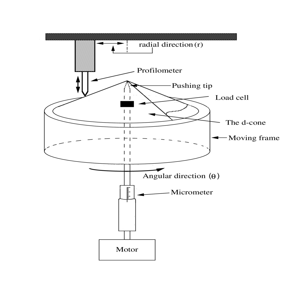
FIG. 1.: The set up where the d-cone is performed and where the profilometric measurements are achieved.

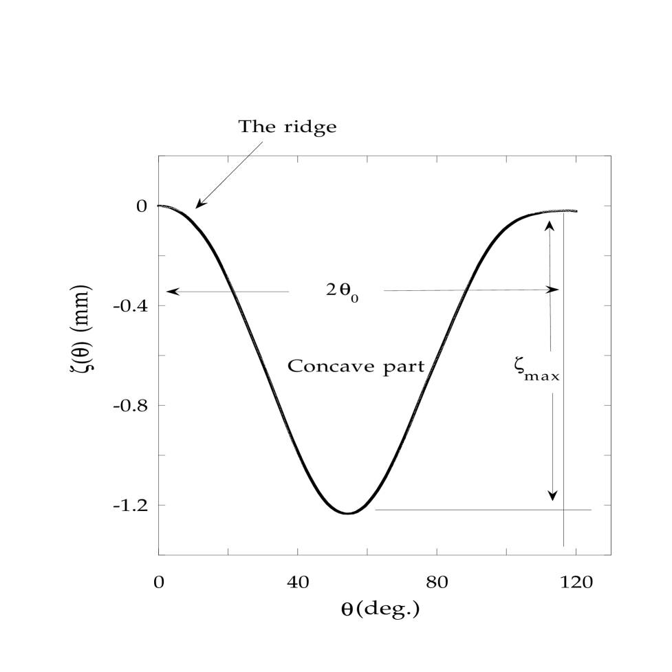
FIG. 2.: The profile of the d-cone in cartesian coordinates. Notice the angle $2\theta_{0}$ that measures the aperture angle between the points where the plate looses contact with the frame

.

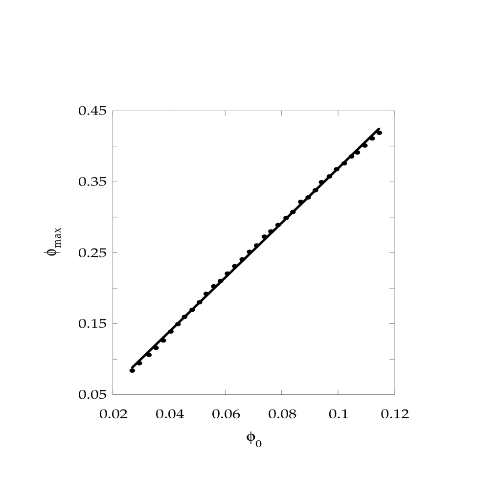
FIG. 3.: The plate maximum deflection as a function of the angle between the convex part and the horizontal. The distance to the pushing tip is 3mm.

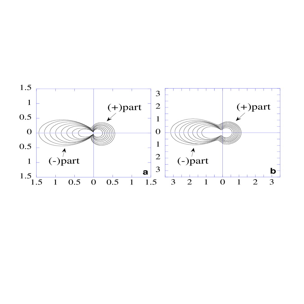
FIG. 4.: The profile of the sheet in polar coordinates vs. the angle $\theta$. a) d=1.41 mm; b) d=5.48 mm. The axis are in mm. The different curves correspondent to different distances to the pushing tip.

FIG. 5.: Geometrical construction of the d-cone obtained after a cut by a plane of a perfect cone

FIG. 6.: The d-cone profiles obtained from the geometrical model. Each curve correspond to a distance from the origin. The distance $x_{s}$ is set to 1. The frame radius is set to 37 mm and the thickness to 0.1 mm. The different distances are $r$=2,4,6,12 (scaled units).

FIG. 7.: The plate height $\tilde{z}_{m}$ obtained from the geometrical model. The parameters are the same as in figure 6. The distance to the tip is 2 scaled units.

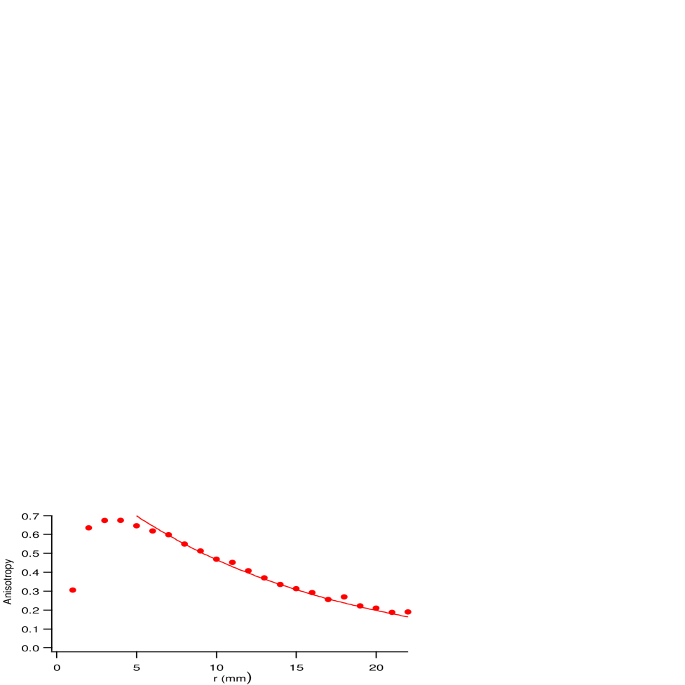
FIG. 8.: The anisotropy $\mathcal{A}$ as a function of the distance r. The deformation is 1.5 mm .

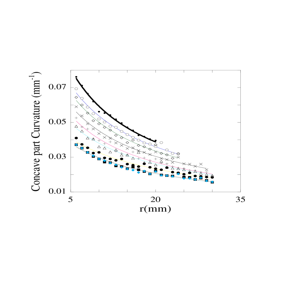
FIG. 9.: The concave-part local curvature vs. the distance to the singularity, and for different small $d$. The line is a best fit to the function $1/(r+r_{s})$.

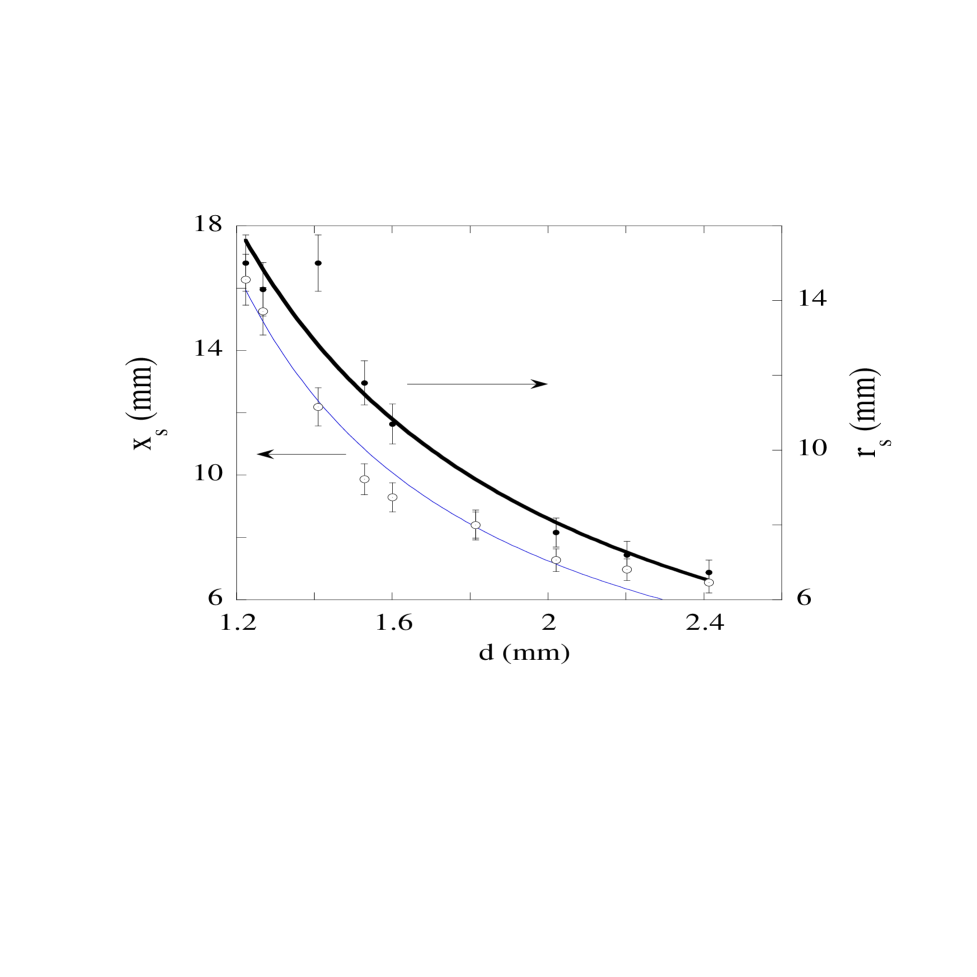
FIG. 10.: The shift distance $r_{s}$ and the singularity displacement $x_{s}$ vs. d

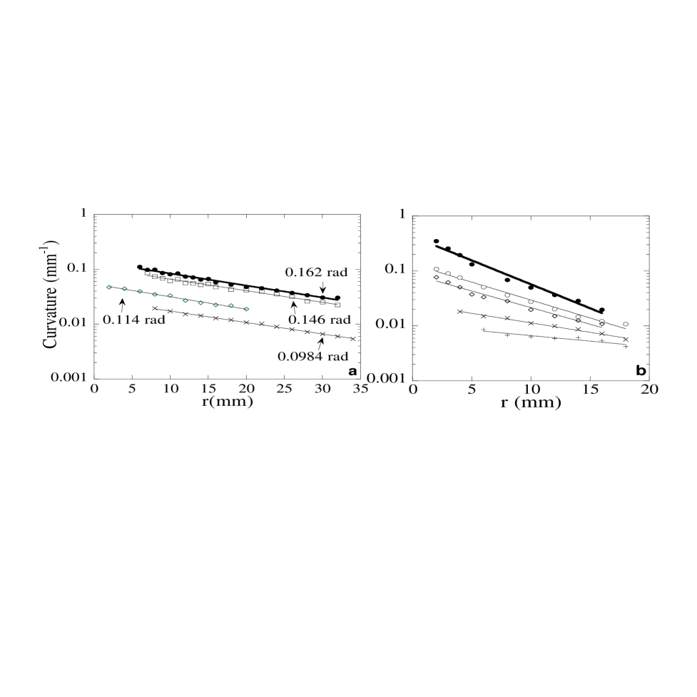
FIG. 11.: The d-cone local curvature vs. the distance r from the pushing tip for different deformations. (a) the local curvature of the concave part, where $r_{c}$ is constant and equal to 20 mm. (b) the ridge local curvature, where $r_{c}$ decreases when $d$ increases. In the figure we reported the values of the opening angle and not d

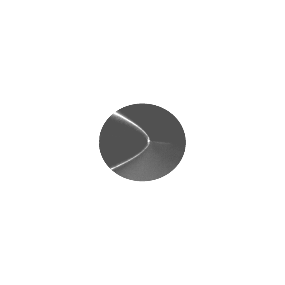
FIG. 12.: The d-cone observed from above, and illuminated perpendicularly to the plane of the bright parabola. The deformation is about 0.3 mm. $R_{f}$=22.5 mm

FIG. 13.: The radius of curvature of the crescent for small $\epsilon$. The line is a best fit to the power law $\epsilon^{-1/3}$

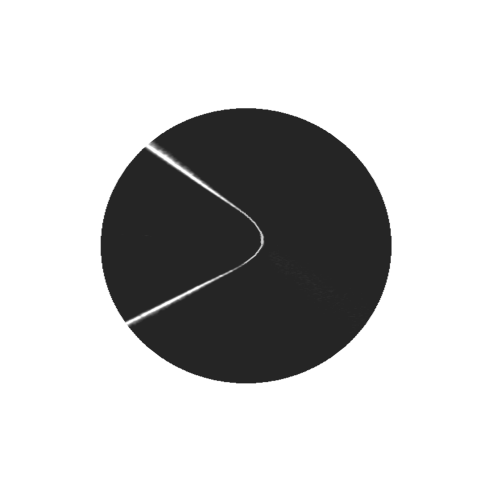
FIG. 14.: Top view of the d-cone at high deformation. The bright line which is no longer a parabola, but a hyperbola and one can notice a distance over which the wings of this line become linear. The deformation is about 7 mm. $R_{f}$=30mm

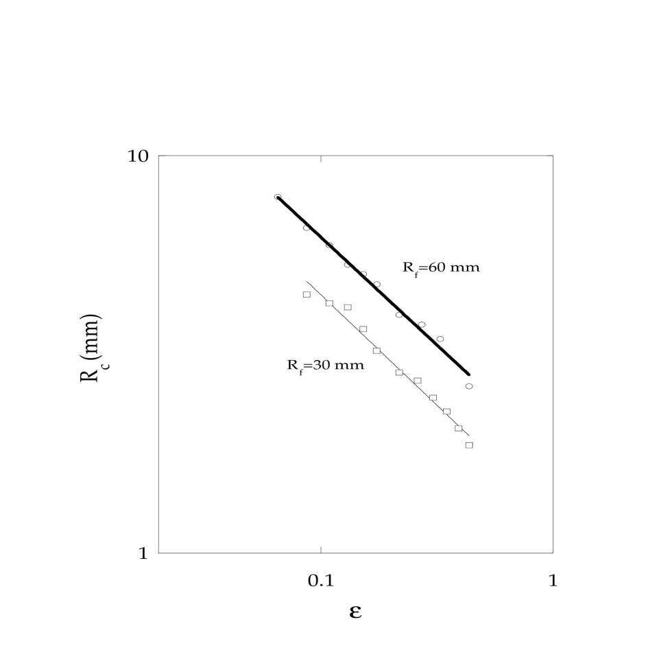
FIG. 15.: The radius of the crescent versus $\epsilon$ for large deformations. The line are best fit to the power law $\epsilon^{-1/2}$

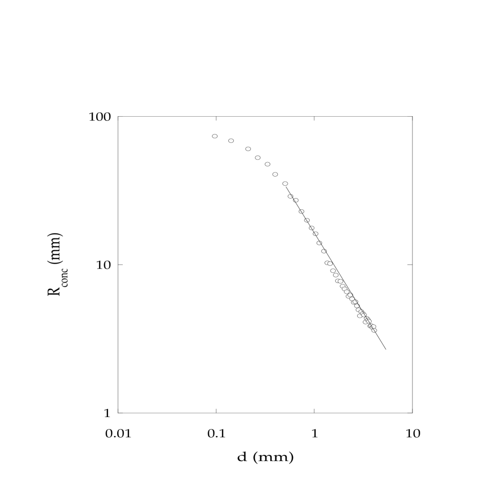
FIG. 16.: The local radius of curvature of the concave region close to the singularity. The line has a slope close to -1.

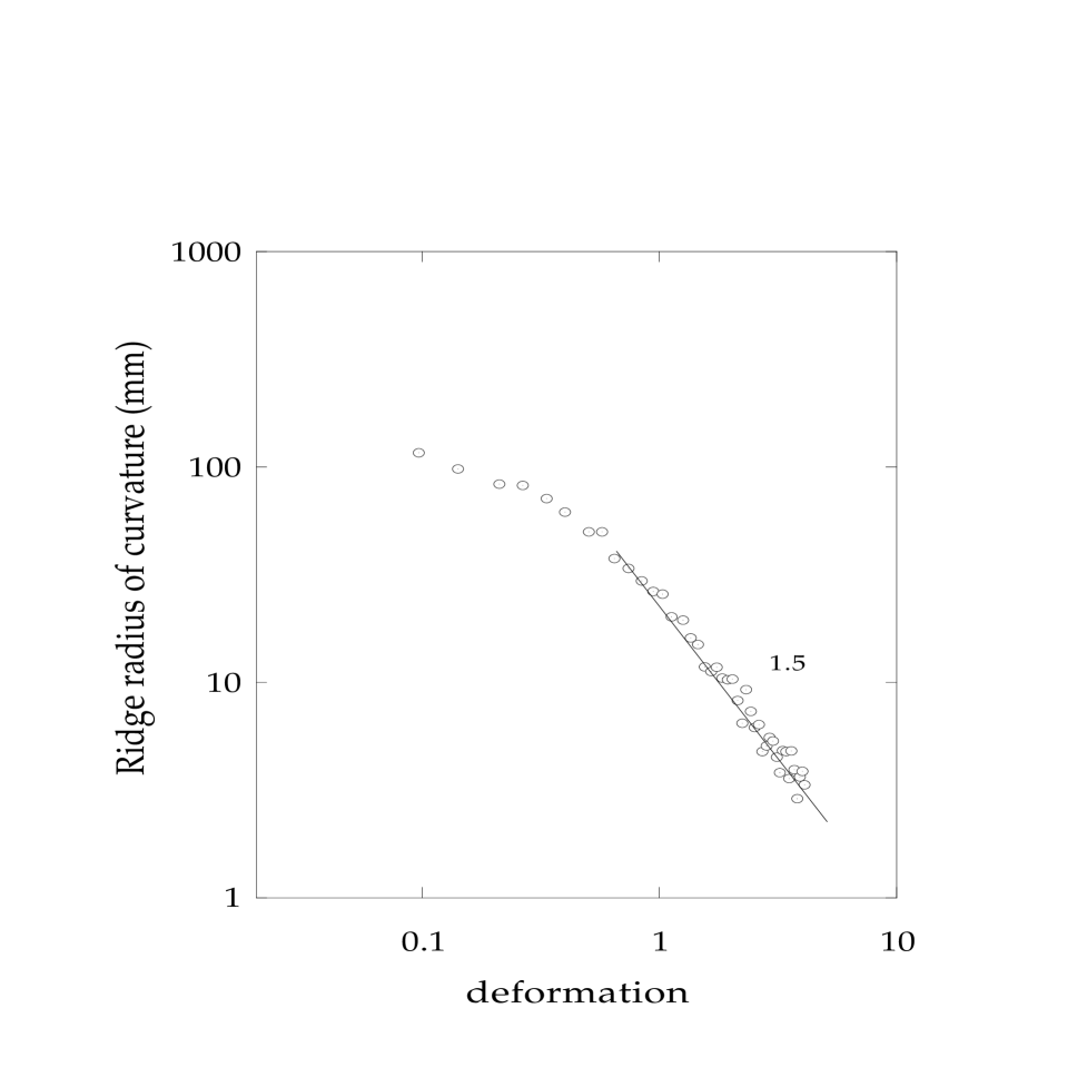
FIG. 17.: The radius of curvature of the ridge as a function of the deformation. The straight line has a slope - 1.5

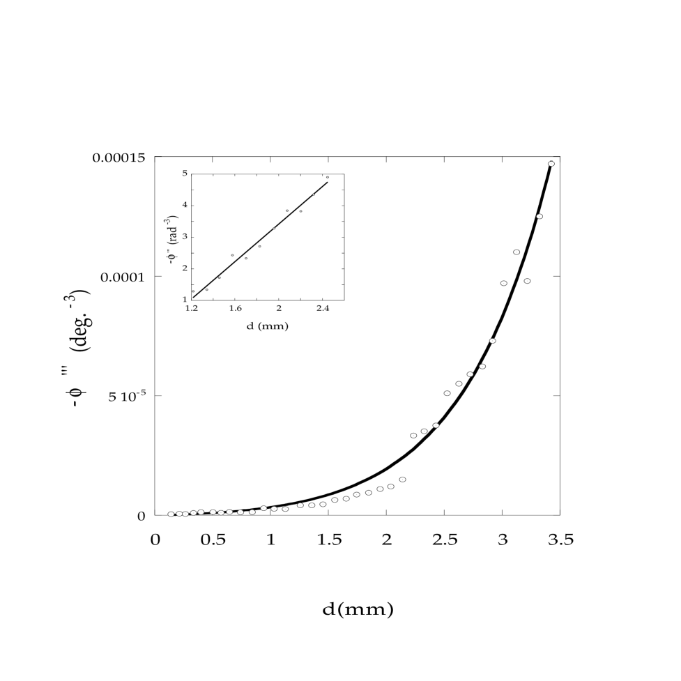
FIG. 18.: The third derivative of the profile ($\phi$) at the ridge as versus the deformation and at a distance of 3 mm from the tip. Inset: the third derivative at a distance of 6 mm from the d-cone tip.

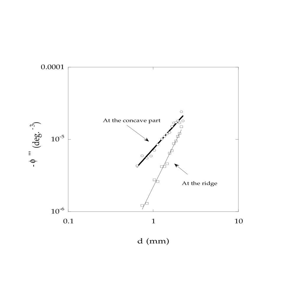
FIG. 19.: The reaction force at the ridge and at the concave part vs. the deformation. The slope of the line giving the force at the ridge is twice larger than the one corresponding to the concave part. The data are taken at 3 mm from the tip.

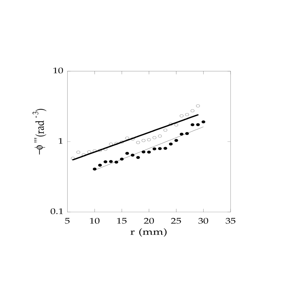
FIG. 20.: The reaction force at the ridge vs $r$. The upper curve corresponds to d=1.9 mm and the lower curve corresponds to d=1.2 mm.

FIG. 21.: Force vs. $\epsilon$ for different frame radius for transparencies. The saturation force increases when the frame radius decreases. For stailess steal, the crossover is an order of magnitude lower. For copper the crossover is 0.05.

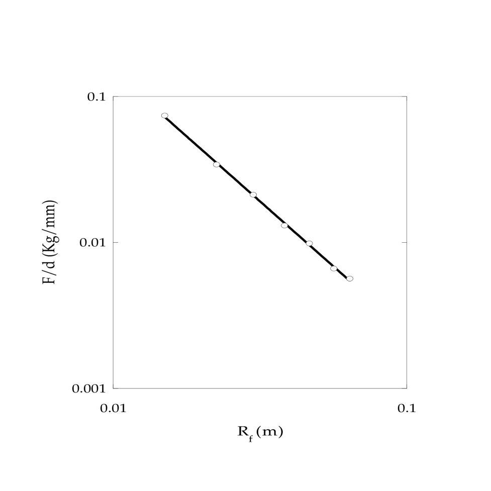
FIG. 22.: The slope of the force in the elastic regime vs. $R_{f}$. The slope of the fitting line is close to 2.

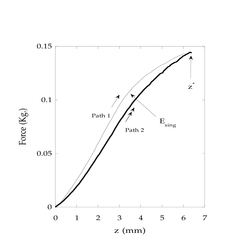
FIG. 23.: The method how the energy of the singularity is measured. Path1 and Path2 are the “crumpling” of a perfectly flat plate and the reloading of the already crumpled plate. The area between the thick line (path2) and the thin line (path1) is the energy of the singularity

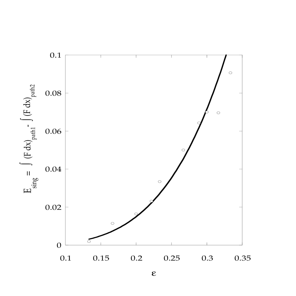
FIG. 24.: The singularity energy, which is the energy necessary to form the scar. The line is the best fit to a power law $\epsilon^{4}$

REFERENCES

- [1] M. Mutz, D. Bensimon, and M.J. Brienne. Phys. Rev. Lett. 67,923 (1991).
- [2] Y. Kantor, M. Kardar and D.R. Nelson, Phys. Rev. Lett. 57, 791 (1986); Statistical Mechanics of Membranes and Surfaces, edited by D. Nelson, T. Piran, and S. Weinberg, (World Scientific, Singapore, 1989).
- [3] D. R. Nelson and L. Peliti, J. Phys. (Paris) 48 1085 (1987); M. Paczuski, M. Kardar and D. R. Nelson, Phys. Rev. Lett. 60 2638 (1988); D. Morse, T. Lubensky and G. Grest, Phys. Rev. A 45 R2151 (1992); D. Bensimon, D. Mukamel and L. Peliti, Europhys. Lett. 18 269 (1992); X. Wen, C. W. Garland, T. Hwa, M, Kardar, E, Kokufuta, Y. Li, M. Orkisz and T. Tanaka, Nature 355 426 (1992); R. Attal, S. Chaïeb, and D. Bensimon. Phys. Rev. E 48 2232 (1993); Y. Park and C, Kwon, Phys. Rev. E 54 3032 (1996).
- [4] M. S. Spector, E. Naranjo and J. A. Zasadzinski, Phys. Rev. Lett. 73 2867 (1994); R. R. Chianelli, E. B. Prestige, T. A. Pecoraro and J. P. DeNeufville, Science 203 1105 (1979).
- [5] M. R. Falvo, G. J. Clary, R. M. Taylor II, V. Chi, F. P. Brooks Jr, S. Washburn and R. Superfine, Nature 389 582 (1997); M. M. Treacy, T. W. Ebbesen and J. M. Gibson, Nature 381 678 (1996); B. I. Yakobson, C. J. Brabec and J. Bernholc, Phys. Rev. Lett. 76 2511 (1996).
- [6] S. Deser, R. Jackiw and G. ’t Hooft, Ann. of Phys. 152, 220 (1984).
- [7] Y. Pomeau, C. R. Acad. Sci. I, Math. 320, 975 (1995);
- [8] A. Lobkovsky, S. Gentges, Hao. Li, D. Morse, and T.A. Witten, Science 270, 1482 (1995).
- [9] M. Ben Amar and Y. Pomeau, Proc. R. Soc. London A, 453,729, (1996).
- [10] T.A. Witten and H. Li, Europhys. Lett. 23, 51 (1993);
- [11] E. M. Kramer and T.A. Witten, Phys. Rev. Lett. 78, 1303 (1997).
- [12] A. Lobkovsky, Phys. Rev. E 53, 3750 (1996);
- [13] A, E. Lobkovsky and T. A. Witten Phys. Rev. E 55, 1577 (1997)
- [14] S. Chaïeb and F. Melo, Phys. Rev. E 56, 4736 (1997).
- [15] S. Chaïeb, F. Melo and J. C. Géminard, Phys. Rev. Lett. 80, 2354 (1998)
- [16] E. Cerda and L. Mahadevan, Phys. Rev. Lett. 80, 2358 (1998).
- [17] S. Chaïeb and J.C. Géminard (in preparation).
- [18] S. Chaïeb and F. Melo in Instabilities and Nonequilibrium Structures VI, Tirapegui and Zeller Eds (1997).
- [19] L. Mahadevan (private communication)
- [20] S. Chaïeb, E. Cerda, F. Melo and L. Mahadevan (in preparation)
- [21] L. Landau and E. Lifchitz, Théorie de l’élasticité. (Mir, Moscow,1967) page 87.
- [22] The term (wing) is introduced in [13] to describe the region where the strain persists although all the energy is concentrated near the singularity.
- [23] P. Oswald (private communication)
.