Numerical Computation of Thermoelectric and Thermomagnetic Effects

Abstract

Phenomenological equations describing the Seebeck, Hall, Nernst, Peltier, Ettingshausen, and Righi-Leduc effects are numerically solved for the temperature, electric current, and electrochemical potential distributions of semiconductors under magnetic field. The results are compared to experiments.

1 Introduction

It is well known that geometry of samples (e.g., ratio of length to width for rectangular samples) affects magnetoresistance. Short samples become more electrically resistant under magnetic field than long ones (see Fig. 3 below).

For the Seebeck and the Nernst effects, experimental evidences for such geometric contribution are not so clear. Ertl [1] measured Bi-Sb alloy samples of various lengths, and showed that longer samples exhibit greater Seebeck coefficients. Measurement of Seebeck coefficient by Ikeda et al [2], however, is not easy to summarize, but their Nernst coefficient of wider (“fat bridge”) sample (Fig. 7) under 4 Tesla was about 12 percent smaller than that of narrower one (Fig. 8).

Though analytic solutions exist for a limited class of the Hall effect [3], numerical computation is necessary to explain these results in general. We developed a two-dimensional numerical simulation code based on phenomenological equations governing thermoelectric and thermomagnetic effects. Section 2 summarizes the basic equations. Sections 3–6 describe the numerical algorithm. Sections 7 and 8 summarizes the results and discuss consequences.

2 Phenomenological Equations

The phenomemological equations governing thermoelectric and thermomagnetic phenomena of solids are [4, 5]

$$-\boldsymbol{\nabla}\phi=\rho\boldsymbol{J}+\alpha\boldsymbol{\nabla}T+R\boldsymbol{B}\times\boldsymbol{J}+N\boldsymbol{B}\times\boldsymbol{\nabla}T$$ (1)

$$\boldsymbol{q}=\phi\boldsymbol{J}-\kappa\boldsymbol{\nabla}T+\alpha T\boldsymbol{J}+NT\boldsymbol{B}\times\boldsymbol{J}+\kappa M\boldsymbol{B}\times\boldsymbol{\nabla}T$$ (2)

where $\phi$ is the electrochemical potential per unit charge, $\rho$ the (isothermal) electric resistivity, $\boldsymbol{J}$ the electric current density, $\alpha$ the (isothermal) Seebeck coefficient, $T$ the temperature, $R$ the (isothermal) Hall coefficient, $\boldsymbol{B}$ the magnetic flux density, $N$ the (isothermal transverse) Nernst coefficient, $\boldsymbol{q}$ the energy flux density, $\kappa$ the (isothermal) thermal conductivity, and $M$ the Righi-Leduc coefficient. In Eq. (1), the last three terms represents the Seebeck, the Hall, and the Nernst effects, respectively. In Eq. (2), the last three terms are responsible for the Peltier/Thomson, the Ettingshausen, and the Righi-Leduc effects, respectively.

In what follows we assume that (1) the system is in steady state, so that $\boldsymbol{\nabla}\cdot\boldsymbol{J}=\boldsymbol{\nabla}\cdot\boldsymbol{q}=0$ holds; (2) the external magnetic field $\boldsymbol{B}$ is independent of the position, and is along the $z$-direction; (3) the electric current $\boldsymbol{J}$ has no $z$-component; (4) the temperature $T$ is independent of the $z$-coordinate; (5) the conductor is homogenious, so that all of the transport coefficients ($\alpha$, $\rho$, $\kappa$, $R$, $N$, $M$) are functions of temperature $T$ alone.

3 Overview of the Method

Our aim is to calculate $T$, $\phi$, and $\boldsymbol{J}$ distributions for rectangular and irregular-shaped semiconductor samples such as shown in Fig. 1.

Figure 1: Example of discretization. This figure corresponds to the “bridge” shape of Ikeda et al [2].

We discretize position by constructing a grid with square meshes of size $h\times h$. We consider $T$ and $\phi$ on each grid points (corners of the meshes), and $\boldsymbol{J}$ on each side of the meshes, as shown in Fig. 2.

Figure 2: Grid point $(i,j)$ and its four adjacent points. Temperature $T_{ij}$ and potential $\phi_{ij}$ are specified on point $(i,j)$, whereas electric current $J_{ij}^{x}$ is specified along the line segment connecting two points $(i,j)$ and $(i+1,j)$.

After setting up suitable initial values for $T$, $\phi$, and $\boldsymbol{J}$, we proceed as follows:

1. On each grid point $(i,j)$, update $T_{ij}$ from the discretized Poisson equation for temperature (see Section 4 below), assuming all the other quantities fixed.

2. On each line segment connecting adjacent grid points, update $\boldsymbol{J}_{ij}$ (see Section 5 below), assuming all the other quantities fixed.

3. On each grid point, update $\phi_{ij}$ so as to satisfy the continuity equation for $\boldsymbol{J}_{ij}$ at the point (see Section 6 below).

4. Go to Step 1.

4 Temperature Updates

The Poisson equation for temperature can be derived by taking the divergence of Eq. (2) and using Eq. (1):

$$\left(\kappa-\frac{N^{2}TB^{2}}{\rho}\right)\nabla^{2}T\\ =-\rho J^{2}+\left(T\frac{d\alpha}{dT}+\frac{NTB^{2}}{\rho}\frac{dR}{dT}\right)(\boldsymbol{\nabla}T)\cdot\boldsymbol{J}\\ +\left(2N+T\frac{dN}{dT}-\frac{NT}{\rho}\frac{d\rho}{dT}\right)(\boldsymbol{\nabla}T)\cdot(\boldsymbol{B}\times\boldsymbol{J})\\ +\left(\frac{NTB^{2}}{\rho}\frac{dN}{dT}-\frac{d\kappa}{dT}\right)(\boldsymbol{\nabla}T)^{2}$$ (3)

This second-order partial differential equation for $T$, which we shall abbreviate as $\nabla^{2}T(x,y)=F(x,y)$, can be discretized as follows: If the point $(i,j)$ is not on the boundary,

$$T^{\mathrm{new}}_{ij}=\frac{T_{i-1,j}+T_{i+1,j}+T_{i,j-1}+T_{i,j+1}}{4}-\frac{h^{2}}{4}F$$ (4)

(with suitable modification to accelerate convergence). On the boundary, either $T_{ij}$ is given (Dirichlet conditions), or derivatives of $T$ in the direction normal to the boundary, $\nabla_{n}T(x,y)$, is given (Neumann conditions). In the latter case, if the grid point $(i,j)$ is on the boundary which is along the $x$-direction such that point $(i-1,j)$ is outside of the sample, the normal derivative $\nabla_{y}T=\partial T/\partial y$ should be given, and the update formula is

$$T^{\mathrm{new}}_{ij}=\frac{T_{i-1,j}+T_{i+1,j}+2T_{i,j+1}-2h\nabla_{y}T}{4}-\frac{h^{2}}{4}F$$ (5)

Similarly, at a corner point such that points $(i-1,j)$ and $(i,j-1)$ are outside of the boundary, the update formula becomes

$$T^{\mathrm{new}}_{ij}=\frac{2T_{i+1,j}+2T_{i,j+1}-2h\nabla_{x}T-2h\nabla_{y}T}{4}-\frac{h^{2}}{4}F$$ (6)

The normal derivative, say $\nabla_{y}T$, can be derived from Eq. (2) if there is no energy and current transfer through the boundary ($q_{y}=J_{y}=0$),

$$\nabla_{y}T=NTB_{z}J_{x}/\kappa+MB_{z}\nabla_{x}T$$ (7)

5 Electric Current Calculation

Given $T$ and $\phi$, the electric current density $\boldsymbol{J}$ can be computed from Eq. (1), which can be written as

$$\rho\boldsymbol{J}+R\boldsymbol{B}\times\boldsymbol{J}=-\boldsymbol{\nabla}\phi-\alpha\boldsymbol{\nabla}T-N\boldsymbol{B}\times\boldsymbol{\nabla}T$$ (8)

or, in coordinate components

$$\begin{pmatrix}\rho&-RB_{z}\\ RB_{z}&\rho\end{pmatrix}\begin{pmatrix}J_{x}\\ J_{y}\end{pmatrix}=\begin{pmatrix}-\nabla_{x}\phi-\alpha\nabla_{x}T+NB_{z}\nabla_{y}T\\ -\nabla_{y}\phi-\alpha\nabla_{y}T-NB_{z}\nabla_{x}T\end{pmatrix}$$ (9)

Hence

$$\begin{pmatrix}J_{x}\\ J_{y}\end{pmatrix}=\frac{1}{\rho^{2}+R^{2}B_{z}^{2}}\begin{pmatrix}\rho&RB_{z}\\ -RB_{z}&\rho\end{pmatrix}\\ \times\begin{pmatrix}-\nabla_{x}\phi-\alpha\nabla_{x}T+NB_{z}\nabla_{y}T\\ -\nabla_{y}\phi-\alpha\nabla_{y}T-NB_{z}\nabla_{x}T\end{pmatrix}$$ (10)

On the boundary, if $J_{y}=0$ holds, then

$$J_{x}=(-\nabla_{x}\phi-\alpha\nabla_{x}T+NB_{z}\nabla_{y}T)/\rho$$ (11)

Furthermore, if $q_{y}=0$ also holds, substitution of (7) into (11) gives

$$J_{x}=\frac{1}{\rho}\left(-\nabla_{x}\phi-(\alpha-NMB_{z}^{2})\nabla_{x}T+\frac{N^{2}B_{z}^{2}TJ_{x}}{\kappa}\right)$$ (12)

Solving for $J_{x}$, we have

$$J_{x}=\left(-\nabla_{x}\phi-(\alpha-NMB_{z}^{2})\nabla_{x}T\right)\biggm{/}\left(\rho-\frac{N^{2}B_{z}^{2}T}{\kappa}\right)$$ (13)

6 Potential Updates

Instead of using a lengthy Poisson equation for the electrochemical potential $\phi$ that can be derived from Eq. (1), we base our calculation of $\phi$ on the continuity equation of electric current, $\boldsymbol{\nabla}\cdot\boldsymbol{J}=0$.

We start with Eq. (10) which has the form

$$J_{x}=\frac{1}{\rho^{2}+R^{2}B^{2}}(-\rho\nabla_{x}\phi-RB_{z}\nabla_{y}\phi)\\ +\text{terms independent of $\phi$}$$ (14)

and similarly for $J_{y}$. As was discussed earlier, the discretized value $J^{x}_{ij}$ is taken along the line segment connecting two points with potentials $\phi_{ij}$ and $\phi_{i+1,j}$. Along this line segment, we can approximate potential derivatives by $\nabla_{x}\phi=(\phi_{i+1,j}-\phi_{ij})/h$ and $\nabla_{y}\phi=(\phi_{i,j+1}+\phi_{i+1,j+1}-\phi_{i,j-1}-\phi_{i+1,j-1})/(4h)$. After these derivatives are substituted, the equation for $J^{x}_{ij}$ above has the $\phi_{ij}$ dependence:

$$J^{x}_{ij}=\frac{\rho\phi_{ij}}{h(\rho^{2}+R^{2}B^{2})}+\text{terms independent of $\phi_{ij}$}$$ (15)

Note that $J^{x}_{ij}$ is the current outgoing from the point $(i,j)$ in the positive $x$-direction. As can be seen from Fig. 2, there are four such expressions outgoing from point $(i,j)$: $J^{x}_{ij}$, $J^{y}_{ij}$, $-J^{x}_{i-1,j}$, $-J^{y}_{i,j-1}$. When these four expressions are added, we arrive at

$$J^{\mathrm{out}}_{ij}=\frac{4\rho\phi_{ij}}{h(\rho^{2}+R^{2}B^{2})}+\text{terms independent of $\phi_{ij}$}$$ (16)

Now, if we replace the value of $\phi_{ij}$ by

$$\phi^{\mathrm{new}}_{ij}=\phi_{ij}-J^{\mathrm{out}}_{ij}h(\rho^{2}+R^{2}B^{2})/(4\rho)$$ (17)

the right-hand side of Eq. (16) will vanish. We use Eq. (17) and similar ones with suitable modification for grid points on the boundary, to update $\phi_{ij}$.

7 Results

We conducted numerical computations on intrinsic indium antimonide (InSb) semiconductor samples with the following properties near 300 K.

$$\begin{array}[]{r@{\;=\;}l@{\;}l}\rho&8.0T^{-5.333}\times 10^{8}&\mathrm{\Omega\,m}\\ R&(-5.6e^{-0.034(T-273)}-0.9)\times 10^{-4}&\mathrm{m^{3}\,A^{-1}\,s^{-1}}\\ \alpha&(-3.2+0.01(T-273))\times 10^{-4}&\mathrm{V\,K^{-1}}\\ N&(-5.7e^{-(T-273)/65}-3.2)\times 10^{-5}&\mathrm{m^{2}\,K^{-1}\,s^{-1}}\\ M&5\times 10^{-2}&\mathrm{m^{2}\,V^{-1}\,s^{-1}}\\ \kappa&1.4\times 10^{5}T^{-1.65}&\mathrm{W\,K^{-1}\,m^{-1}}\end{array}$$ (18)

These values are not meant to be good fits to measurements. They are only shown here as example inputs to our code. (In fact, $\rho$, $\alpha$, and $N$ are rough fits to measurements near 300 K by Ikeda and others [2, 6, 7], but the conditions are not uniform: $N$ is measured under 4 Tesla, whereas $\alpha$ under no magnetic field.)

On the basis of these values, we computed magnetoresistance and Seebeck and Nernst effects with various sample geometry.

The magnetoresistance results (Fig. 3) are in good agreement with experiment ([8], Fig. 4.8 of Seeger [9]).

Figure 3: Simulation results of magnetoresistance for intrinsic InSb semiconductor with different geometry: length ($x$-direction) $\times$ width ($y$-direction) $=$ 10 mm $\times$ 1 mm, 10 mm $\times$ 10 mm, and 4 mm $\times$ 12 mm, with negligible thickness ($z$-direction). External magnetic field is along the $z$-direction.

Seebeck and Nernst coefficients should vary much with the magnetic field, so the results for these coefficients are to be compared with those of different geometry under the same magnetic field.

As Fig. 4 shows, the Seebeck effect is not sensitive to geometry if current leads that measure longitudinal voltage difference are narrow enough. On the other hand, if current leads are as wide as the sample width, Seebeck effect degrades and can even change sign for short samples. This tendency explains some experimental evidence for the size dependence of magneto-Seebeck effect [1].

Similar tendency can be seen in Fig. 5 for the Nernst effect. In this case, however, geometry effect exists even with narrow current leads. This is because the Righi-Leduc effect causes transverse ($y$-direction) temperature gradient that is proportional to the magnetic field $B$. This transverse temperature gradient in turn causes transverse voltage gradient by the Seebeck effect. When divided by $B$, this transverse voltage gives a nearly constant bias to the apparent Nernst coefficient.

This effect partly explains what Ikeda et al [2] found out: Under 4 Tesla the apparent Nernst coefficient for their “fat bridge” (wide with legs) sample (Fig. 7) is about 12 percent smaller than those of narrower one (Fig. 8), whereas our simulation gives only 7 to 8 percent smaller coefficient. Though they are careful to make their current leads narrow, inevitable finite widths of the leads might explain further effect.

Figure 4: Simulation results of apparent Seebeck coefficient for intrinsic InSb samples with different geometry. Apparent Seebeck coefficient is defined to be $\alpha_{\mathrm{eff}}=\Delta_{x}\phi/\Delta_{x}T$, where $\Delta_{x}\phi$ is longitudinal potential difference, and $\Delta_{x}T$ is longitudinal temperature difference. Solid lines: Current leads are of negligible widths, Dashed lines: Current leads are as wide as the sample widths.

Figure 5: Simulation results of apparent Nernst coefficient for intrinsic InSb samples with different geometry. Apparent Nernst coefficient is defined to be $N_{\mathrm{eff}}=L\Delta_{y}\phi/BW\Delta_{x}T$, where $\Delta_{y}\phi$ is transverse potential difference, $\Delta_{x}T$ longitudinal temperature difference, $L$ length (in $x$-direction), $W$ width (in $y$-direction), and $B$ magnetic induction. Solid lines: Current leads are of negligible widths, Dashed lines: Current leads are as wide as the sample widths.

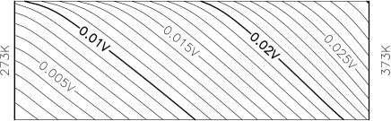
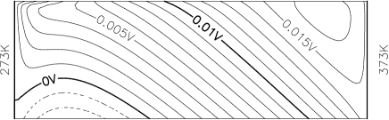
Figure 6: Contour maps of calculated potential distribution for a 12 mm $\times$ 4 mm sample in 4-Tesla magnetic field. Upper: Current leads are of negligible width. Lower: Current leads are as wide as the sample width. The left and the right edges are kept at 273 K and 373 K, respectively.

Figure 7: Contour map of calculated potential distribution for “fat bridge” sample of Ikeda et al [2].

Figure 8: Contour map of calculated potential distribution for “bridge” sample of Ikeda et al.

8 Discussion

As can be seen from the contour maps, the potential distributions of thermomagnetic samples are rather complicated. They change dramatically with different sample geometry. Moreover, if we attach current leads of finite widths to the cold and hot edges, much of the transverse voltage gradient is shorted out, resulting in quite a different potential distribution. To correct for such a bias, careful numerical calculation is necessary.

Inspection of Fig. 6 (upper) and Fig. 7 shows that the best way to generate electricity from wide samples under magnetic field is to attach current leads to the bottom left and the top right corners. In this way, we can utilize both the Seebeck and the Nernst effects.

Figs. 7 and 8 also show that at the far end of a small “leg,” potential gradient along the boundary decreases by an order of magnitude or more, thus making measurement of Nernst coefficients less prone to the widths of current leads.

References

- [1] M. E. Ertl, G. R. Pfister, and H. J. Goldsmid, Size dependence of the magneto-Seebeck effect in bismuth-antimony alloys, Brit. J. Appl. Phys. 14, 161 (1963).
- [2] K. Ikeda, H. Nakamura, and S. Yamaguchi, Geometric contribution to the measurement of thermoelectric power and Nernst coefficient in a strong magnetic field, ICT97, Dresden, Germany (1997); http://xxx.lanl.gov/abs/cond-mat/9709152 (1997).
- [3] R. F. Wick, Solution of the Field Problem of the Germanium Gyrator, J. Appl. Phys. 25, 1741 (1954).
- [4] L. D. Landau, E. M. Lifshitz and L. P. Pitaevskiĭ, Electrodynamics of Continuous Media, 2nd ed., Butterworth-Heinemann, 1984.
- [5] T. C. Harman and J. M. Honig, Thermoelectric and Thermomagnetic Effects and Applications, McGraw-Hill, 1967.
- [6] K. Ikeda, H. Nakamura, S. Yamaguchi, and K. Kuroda, Measurement of transport properties of thermoelectric materials in the magnetic field, J. Adv. Sci., 8 (1996), 147 (in Japanese).
- [7] H. Nakamura, K. Ikeda, S. Yamaguchi, and K. Kuroda, Transport coefficients of thermoelectric semiconductor InSb in the magnetic field, J. Adv. Sci., 8 (1996), 153 (in Japanese).
- [8] H. Welker and H. Weiss, Z. Phisik 138, 322 (1954).
- [9] K. Seeger, Semiconductor Physics: An Introduction, sixth edition, Springer, 1997.