Theory and data analysis for excitations in liquid ⁴He beyond the roton minimum

Abstract

The hybridization of the single-excitation branch with the two-excitation continuum in the momentum region beyond the roton minimum is reconsidered by including the effect of the interference term between one and two excitations. Fits to the latest experimental data with our model allow us to extract with improved accuracy the high momentum end of the ⁴He dispersion relation. In contrast with previous results we find that the undamped excitations below two times the roton energy survive up to $Q=3.6$ Å^-1 due to the attractive interaction between rotons.

PACS numbers: 67.40.Db, 61.12.-q

Although excitations in superfluid ⁴He have been widely studied in the last decades (see for instance Ref. [2, 3]), the nature of the single particle spectrum termination remains unclear. Forty years ago, Pitaevskii predicted different kinds of termination depending on the detailed form of the spectrum at low momenta [4]. In the case of a decay into pairs of rotons, Pitaevskii theory describes the avoided crossing of the bare one-excitation branch with the continuum of two excitations. Within this picture the low energy pole is repelled by the continuum, so that the spectrum flattens out for large $Q$ towards 2$\Delta$ losing spectral weight ($\Delta$ is the roton energy). At the same time, a damped excitation for $\omega>2\Delta$ appears and shifts to higher energies. Neutron scattering experiments later suggested that the decay of excitations into pairs of rotons did actually take place for momentum $Q\gtrsim 2.6$ Å^-1 [5]. The flattening of the spectrum at an energy of the order of $2\Delta$ being the main feature in support of Pitaevskii’s picture. Despite the good qualitative agreement between theory and experiment, several issues addressed by the theory could not be verified due to insufficient instrumental resolution. In particular, theory predicts a singular termination of the spectrum at a definite value of momentum $Q_{c}$ for a repulsive interaction ($V_{4}>0$) between rotons. In the case of an attractive interaction, hybridization between the roton bound state and the single quasiparticles is instead expected, as proposed by Zawadowski-Ruvalds-Solana (ZRS) [6], with the consequence that an undamped quasiparticle peak at an energy slightly below 2$\Delta$ should be present [6, 7, 8, 9]. To our knowledge it has not yet been possible to distinguish clearly between these two cases.

Smith et al. [10] performed the first complete experimental analysis for $2.7\leq Q\leq 3.3$ Å^-1. Although they found indications of a repulsive interaction ($V_{4}>0$) using ZRS theory, they pointed out that the experimental finding of energies for the quasiparticle peak above $2\Delta$ was not accounted for by the theory with reasonable values of the parameters. As a matter of fact, the position of the low-energy peak was not extracted from the data with ZRS theory, but rather by fitting a Gaussian peak on a background of constant slope. The resulting spectrum reached values above $2\Delta$, in contrast with theoretical predictions. From the theoretical point of view it is not possible to explain in a simple way the presence of sharp peaks at energies above $2\Delta$, as the corresponding excitation should be unstable towards decay into two rotons. Moreover, the experimental finding of a repulsive interaction disagrees with different theoretical calculations that predict a negative value for $V_{4}$[11, 8]. More recent experimental investigations by Fåk and coworkers [12, 13] concentrate on the interesting temperature dependence of the dynamical structure factor $S({\bf Q},\omega)$ and do not address directly the issue of the quasiparticle energy or the interaction potential between rotons. In any case they show clearly that there is a strong correlation between the low-energy peak and the high energy continuum as $Q$ increases from 2.3 to 3.6 Å^-1[13], thus indicating that hybridization takes place. We further recall that this hybridization is expected as direct consequence of Bose condensation as explained in details in Ref. [2].

From the theoretical point of view, we recall that the validity of Pitaevskii and ZRS theories is restricted to a small region around 2$\Delta$. Indeed Pitaevskii in his original paper [4] exploited the logarithmic divergence appearing in the two-roton response function [$F_{o}({\bf Q},\omega)=i\,\int{d\omega^{\prime}\over 2\pi}\int{d^{3}{\bf Q}^{\prime}\over(2\pi)^{3}}{\cal G}(p-p^{\prime}){\cal G}(p^{\prime})$, where ${\cal G}^{-1}(p)=\omega+i\,0^{+}-\omega({\bf Q})$, $\omega({\bf Q})$ is the measured spectrum and $p=({\bf Q},\omega)$] to solve exactly the many-body equations. This elegant theory provides explicit expressions for the Green and the density-density correlation functions, valid only in the small energy range where the singularity dominates. This fact leads to problems in data analysis when $Q$ grows so that the bare excitation energy $\omega_{o}({\bf Q})$ takes values above $2\Delta$. In fact, the signal around $2\Delta$ strongly decreases with $Q$ and spectral weight shifts to higher energies following $\omega_{o}({\bf Q})$. To understand the correlation between the high energy part of the spectrum and the one-excitation contribution, it is necessary to extend the validity of the theory to a wider range of energies in order to describe properly the continuum contribution to $S({\bf Q},\omega)$. It then becomes crucial to consider the effect of the direct excitation of two quasiparticles by the neutron and its interplay with the one-quasiparticle excitations usually considered.

The aim of the present paper is to construct such an extension of the theory to describe experimental data for $S({\bf Q},\omega)$ at very low temperatures. Since excitations in ⁴He are stable ($\Gamma({\bf Q})/\omega({\bf Q})\approx 10^{-2}$ for rotons at $1.3$ K with $\Gamma$ the half width of the excitation), it is an excellent approximation to write the Hamiltonian directly in terms of the creation and destruction operators $b^{\dagger}$ and $b$ of these excitations:

$$H_{o}=\sum_{{\bf p}}\omega_{o}({\bf p})b^{\dagger}_{{\bf p}}b^{\phantom{{\dagger}}}_{{\bf p}}+V_{3}\sum_{{\bf p},{\bf q}}\left[b^{\dagger}_{{\bf p}}b^{{\dagger}}_{{\bf q}}b^{\phantom{{\dagger}}}_{{\bf p}+{\bf q}}+cc\right].$$ (1)

We consider for the moment only the $V_{3}$ interaction that induces the hybridization of the single with the double excitation. In general this vertex will be a function of two momenta, for instance the total momentum of the two particles and the momentum of one of them. We neglect from the outset this dependence on momentum as it is expected to be smooth in the region of interest and less important than the frequency dependence retained in the following. Since $S({\bf Q},\omega)$ is the imaginary part of the density-density response function [$\chi({\bf Q},\omega)$] it is convenient to express the density operator $\rho_{{\bf p}}$ in terms of the $b$ and $b^{{\dagger}}$ field operators. In general this will be an infinite series in the $b$-fields, by retaining only the one and two quasi-particle terms we obtain:

$$\rho_{\bf p}=\alpha({\bf p})\left[b^{\dagger}_{{\bf p}}+b^{\phantom{{\dagger}}}_{-{\bf p}}\right]+\sum_{{\bf q}}\gamma({\bf p},{\bf q})\,b^{{\dagger}}_{{\bf p}+{\bf q}}b^{\phantom{{\dagger}}}_{{\bf q}}$$ (2)

$$+\sum_{{\bf q}}\beta({\bf p},{\bf q})\left[b^{\dagger}_{{\bf p}+{\bf q}}b^{\dagger}_{-{\bf q}}+b^{\phantom{{\dagger}}}_{{\bf q}}b^{\phantom{{\dagger}}}_{-{\bf p}-{\bf q}}\right].$$ (3)

Eq. (3) gives the most general second order form for $\rho_{\bf p}$ in terms of $b$ and $b^{\dagger}$ that fulfills parity, time-reversal, and $\rho_{\bf p}^{\dagger}=\rho_{-{\bf p}}$ transformation properties. For the same invariances the three functions introduced $\alpha$, $\beta$, and $\gamma$ are bound to be real. Although the above expression for $\rho_{\bf p}$ is quite general it can be obtained microscopically within a particular approximation scheme [14].

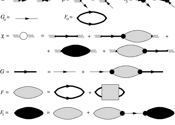
FIG. 1.: Full lines stands for the exact Green function, dashed boxes for the sum of all one-particle irreducible diagrams, and the black box for the sum of all diagrams with two lines closing at the two ends. $\chi(p)$ is the sum of all diagrams with two density insertions (wiggly lines).

It is possible at this point to calculate perturbatively $\chi({\bf Q},\omega)$ using the explicit form of $\rho_{\bf p}$ given in Eq. (3) and the Hamiltonian (1). At zero temperature the contribution of the $\gamma({\bf p},{\bf q})$ term to $\chi$ vanishes, while the momentum dependence of $\alpha({\bf p})$ and $\beta({\bf p},{\bf q})$ is neglected for the sake of simplicity. The diagrammatic theory for the model is shown in Fig. 1 together with the definition of $\chi(p)$, $F_{o}(p)$, $F_{t}(p)$, $F(p)$, and ${\cal G}_{o}(p)=[\omega-\omega_{o}({\bf Q})]^{-1}$. In this figure dashed boxes represent the sum of all one-particle irreducible diagrams. $F_{t}$ stands for the sum of all diagrams with two lines closing at the two ends, and $F$ is the self-energy without the two external couplings. Since the momentum dependence of the vertices is neglected, the Dyson equations for ${\cal G}$ and $F_{t}$ (see Fig. 1) take the simple form of a coupled algebraic system:

$${\cal G}(p) = {\cal G}_{o}(p)+{\cal G}_{o}(p)\,V_{3}\,F(p)\,V_{3}\,{\cal G}(p),$$ (5)

$$F_{t}(p) = F(p)+F(p)\,V_{3}\,{\cal G}_{o}(p)\,V_{3}\,F_{t}(p).$$ (6)

By solving Eqs. (1) and substituting ${\cal G}$ and $F_{t}$ into the expression for $\chi(p)$ we finally obtain:

$$\chi(p)={\alpha^{2}+2\alpha\beta V_{3}F(p)+\beta^{2}F(p)\,{\cal G}_{o}^{-1}(p)\over{\cal G}_{o}^{-1}(p)-V_{3}^{2}\,F(p)}.$$ (7)

Eq. (7) is the basic expression that we will use in the following for the fits to the data [$S({\bf Q},\omega)=-{\rm Im}\chi({\bf Q},\omega)$]. The presence of a $V_{4}$ interaction does not change the above treatment since no $V_{4}$ vertex can connect $F$ to ${\cal G}$ at zero temperature. This implies that the additional diagrams due to a $V_{4}$ interaction contribute only to $F$. Since the explicit calculation of $F$ is difficult and in general depends on the detailed structure of the vertex functions, we prefer to extract it directly from data by exploiting the large (energy and momentum) region of validity of Eq. (7). We proceed by noting that in Eq. (7) only $F$ and $\omega_{o}$ (through ${\cal G}_{o}$) depend on $Q$. Explicit evaluation of $F_{o}$ suggests that the momentum dependence of $F$ should not be pronounced in the range of interest 2.3-3.2 Å^-1. We thus drop this dependence completely in $F$ and fit the resulting function $F(\omega)$ to the data. The $Q$-dependence of $\omega_{o}$ is not negligible because it drives $\omega_{o}(Q)$ through the $2\Delta$ line. In this way we are left with only one parameter dependent on $Q$. It is now possible to extract both $\omega({\bf Q})$ and $F(\omega)$ by fitting Eq. (7) to all sets of data of different momentum at the same time. This procedure exploits fully the information contained in the data because it is sensitive to the correlation among sets with different $Q$. For this reason we are able to extract information for $\omega({\bf Q})$ and for the function $F(\omega)$ over a scale (slightly) smaller than the instrumental resolution.

A few words are necessary to explain how we can find the complex function $F(\omega)$ from the data. The imaginary and real part of $F$ are related by the relation ${\rm Re}F(\omega)=-{1/\pi}{\cal P}\int d\omega^{\prime}{\rm Im}F(\omega)/(\omega-\omega^{\prime})$. We thus need only to parametrize one of them, we choose ${\rm Im}F(\omega)$, since on this function it is easier to apply the physical constraint that excitations are kinematically stable for energies smaller than 2$\Delta$. This condition reads ${\rm Im}F(\omega)=0$ for $\omega<2\Delta$ (the small spectral density between $\omega({\bf Q})$ and $2\Delta$ can be neglected). A simple way to parametrize the function ${\rm Im}F$ is then to choose a set of values of $\omega$ say $\{\omega_{1},\omega_{2},\dots,\omega_{N}\}$ with $2\Delta=\omega_{1}<\omega_{2}<\dots<\omega_{N}$ reasonably spaced and to assign a free parameter, $a_{i}$, to each of them. ${\rm Im}F(\omega)$ can then be defined as a cubic spline interpolation on such a set. The integral to calculate the real part can be performed analytically so that its evaluation is fast and reliable also near the logarithmic singularity at the threshold.

FIG. 2.: Fit to the data from Ref. [12] with a parametrized ${\rm Im}f$. In the inset the resulting ${\rm Im}f$ is shown compared with ${\rm Im}F_{o}$ averaged over $2.3<Q<3.2$ Å^-1 and properly scaled.

We take advantage of a symmetry in Eq. (7) to define a dimensionless function $f(\omega)=\lambda F(\omega)$, constrained by the normalization condition $\int_{2\Delta}^{\omega_{N}}d\omega{\rm Im}f(\omega)=\omega_{N}-2\Delta$. We thus define $g_{3}=V_{3}/\lambda^{1/2}$, and $\tilde{\beta}=\beta/(\lambda^{1/2}\alpha)$. In this way $\alpha$, $\tilde{\beta}$, $g_{3}$, and the $N-1$ parameters that define $f$ are independent and can be fitted to the data. We set ${\rm Im}f(\omega)=a_{N}$ for $\omega>\omega_{N}$ and subtract out the infinite constant that would appear in ${\rm Re}F(\omega)$.

We thus fitted Eq. (7) (convolved with the known instrumental resolution) to experimental data of Ref. [13] (at 1.30 K) by minimizing numerically $\chi^{2}$ for the parameters: $\alpha$, $\tilde{\beta}$, $g_{3}$, $\omega({\bf Q}_{1})$, $\dots$, $\omega({\bf Q}_{n})$, $a_{1}$, $\dots$, $a_{N-1}$ ($N=15$ for the fit presented). The minimization procedure has been performed with different standard routines and the result turned out to be independent of the choice of $\{\omega_{i}\}$ and the initial value of $a_{i}$. A typical starting point for ${\rm Im}f$ is simply $a_{i}=1$ for all $i$. The resulting fit is shown in Fig. 2. Good agreement between theory and experiment is obtained with a reduced $\chi^{2}$ ($\chi^{2}_{R}$) of nearly 4, thus indicating that even if we are leaving a large freedom in $f$ the agreement is significant.

Our main result is summarized by the dispersion relation for the undamped excitation shown in Fig. 3, where it is compared with the one reported in Ref. [15]. We find that the model can quantitatively explain that the peak position of $S(Q,\omega)$ is slightly larger than $2\Delta$ for $Q>2.6$ Å^-1. This originates from a mixing within the instrumental resolution of the contribution of the sharp peak at energy $\omega_{Q}$ slightly smaller than 2$\Delta$ with that of the continuum of two rotons excitations starting at $2\Delta$. On general grounds the continuum should depend strongly on $\omega$ near $2\Delta$, as for $\omega>2\Delta$ there are much more states available to decay into. For these reasons, the assumption of a background of constant slope, used to obtain the values of Ref. [15], is not valid in this momentum region. Our procedure exploits instead the theoretical model for $\chi(p)$ to extract the value of $\omega_{Q}$. In this way we can find the final part of the dispersion relation with improved accuracy and it turns out that data agree with a dispersion relation for the excitations always below 2$\Delta$.

FIG. 3.: Dispersion relation found in the present work (solid line), and in Ref. [4,14] (dashed line). The inset shows the complete dispersion relation.

The importance of the fitted parameter $\tilde{\beta}$ has been checked by studying the function $\chi^{2}(\tilde{\beta})$, where all the other parameters are properly modified to minimize $\chi^{2}$ for each value of $\tilde{\beta}$. The confidence region for $\tilde{\beta}$, i.e. the values of $\tilde{\beta}$ such that $\chi^{2}(\tilde{\beta})/\chi^{2}_{\rm min}<1.5$, turns out to be $-0.17<\tilde{\beta}<-0.01$ meV^-1/2 with a best value $\tilde{\beta}=-0.06$ meV^-1/2. This implies that the direct excitations of two quasiparticles by the neutron gives a small but sizable contribution to $S({\bf Q},\omega)$. Concerning the other parameters we find $\alpha^{2}=1.4$ and $g_{3}=0.8$ meV^1/2.

The shape of ${\rm Im}f$ found by the fit has two main features: a clear peak at $\omega\approx 2$ meV and a “quasi-divergent” behavior at the threshold. The peak is due to the maxon-roton van Hove singularity. This can be verified by comparing the function ${\rm Im}F_{o}(Q,\omega)$, averaged over $2.3\leq Q\leq 3.2$ Å^-1and properly scaled, with the fitted ${\rm Im}f(\omega)$ (see the inset of Fig. 2). Hence it is clear that the peak corresponds in shape and position to the maxon-roton singularity. It is remarkable that no trace of the peak is apparent in any of the experimental plots. It is only by exploiting the correlation between plots with different $Q$ that we have been able to extract this information. On this basis, using the fitted parameters it is also possible to predict that a peak and its shape should be observable with a resolution of $0.1$ meV (to be compared with $0.5$ meV of Fig. 2).

The quasi-singularity at threshold can be understood as an interaction effect, namely a signature of the attractive interaction between rotons. As a matter of fact, in the small region of energy near the threshold we can apply Pitaevski-ZRS [4, 6, 7] theory to evaluate $F(\omega)$ that reads:

$$F({\bf Q},\omega)=4\rho\,\ln{2\Delta-\omega\over D}\left(1-g_{4}\ln{2\Delta-\omega\over D}\right)^{-1},$$ (8)

where $\rho=-{\rm Im}F_{o}({\bf Q},\omega=2\Delta^{+})/2\pi$ is the threshold density of states, $g_{4}=2V_{4}\rho$, and $D$ is a cutoff that can be set to 1 meV as changes in $D$ can be easily reabsorbed in small variations of $\omega_{o}$, $g_{3}$, and $g_{4}$. One can thus readily verify that with a negative value of $g_{4}$ Eq. (8) gives a ${\rm Im}F$ that for $\omega\rightarrow 2\Delta^{+}$ reproduces qualitatively ${\rm Im}f$ of Fig. 2. To verify quantitatively this fact and to find an estimate of $g_{4}$ we have repeated the data fit using Eq. (8) to parametrize $f(\omega)$, (instead of the spline parametrization) and setting a cutoff in energy at $2\Delta$+0.2 meV, in such a way to apply Eq. (8) only where it is supposed to hold. The resulting $\chi^{2}_{R}=1.7$ for the fit gives evidence that the theory works quantitatively in this region and we get for the interaction parameter $V_{4}=g_{4}/(2\rho)\approx-4.7$ meV ų ($g_{4}=-0.15$). The bound-state energy that we obtain from Eq. (8) is indeed very small $E_{B}=D\,\exp\{1/g_{4}\}\approx 1.3\mu eV$. This second fit gives also an additional estimate of the dispersion relation that agrees with the previous one and confirms that an undamped state is present up to $Q=3.6$ Å^-1. The confidence region for $g_{4}$ is $-0.22<g_{4}<-0.08$, restricting $\tilde{\beta}$ to its confidence region already found, which indicates that the interaction is definitely attractive.

Some final comments are in order. First, while Fig. 2 shows the fit for $2.3\leq Q\leq 3.2$, the inclusion of the additional set of data for $Q=3.6$ increases slightly $\chi_{R}^{2}$ (since the momentum range over which we are assuming the vertices to be momentum-independent may be too large) but it remains in any case a good fit to data. For this reason we report in Fig. 3 the value for $\omega({\bf Q})$ obtained in this way. Second, we studied the cutoff dependence of $\chi^{2}_{R}$ when $f(\omega)$ is parametrized according to Eq. (8) and we found that it is very weak up to $\omega=2$ meV where the effect of the maxon-roton peak becomes important. Thus use of the Pitaevskii-ZRS theory for $F$ in our expression (7) does not give a good description of the data if the cutoff in energy is removed. This indicates that the maxon-roton structure and, in general, the whole shape of ${\rm Im}f$ plays a crucial role in determining $S({\bf Q},\omega)$.

In conclusion, we presented a theory for $S({\bf Q},\omega)$ that takes into account both one- and two-quasiparticle excitations by the neutron. The theory reproduces the experimental result over a large range of energy and momentum. We have thus been able to extract the final part of the spectrum dispersion relation in ⁴He. Our theory can be regarded as an extension of the Pitaevskii-ZRS theory taking into account the effect of two-particle excitations. Moreover the range of validity is enlarged as we make no hypothesis on the $F$ function, but we extract it directly from data. In the region where Pitaevskii-ZRS theory holds we have used it to parametrize $F$ in Eq. (7) and we found that the interaction potential among rotons ($V_{4}$) is attractive in this momentum region.

I am indebted to P. Nozières for suggesting this problem to me and for many discussions. I gratefully acknowledge B. Fåk for discussions and critical reading of the manuscript. I acknowledge B. Fåk and J. Bossy for letting me use their data prior to publication. I also thank N. Cooper, N. Manini, A. Würger, P. Pieri, G.C. Strinati, and H.R. Glyde for useful discussions.

REFERENCES

- [1] electronic address: pistoles@ill.fr.
- [2] A. Griffin, Excitations in a Bose-Condensed Liquid (Cambridge University Press, Cambridge, UK, 1993).
- [3] H. R. Glyde, Excitations in Liquid and Solid Helium (Oxford University Press, Oxford, UK, 1994).
- [4] L. P. Pitaevskii, Sov. Phys.-JETP 36, 830 (1959).
- [5] R. A. Cowley and A. D. B. Woods, Can. J. Phys. 49, 177 (1971).
- [6] J. Ruwalds and A. Zawadowski, Phys. Rev. Lett. 25, 333 (1970). A. Zawadowski, J. Ruvalds, and J. Solana, Phys. Rev. B 5, 399 (1972).
- [7] L. P. Pitaevskii, JETP Lett. 12, 82 (1970).
- [8] K. Bedell, D. Pines, and A. Zawadowski, Phys. Rev. B 29, 102 (1984).
- [9] K. J. Juge and A. Griffin, J. Low. Temp. Phys. 97, 105 (1994).
- [10] A. J. Smith et al., J. Phys. C 10, 543 (1977).
- [11] D. K. Lee, Phys. Rev. 162, 134 (1967).
- [12] B. Fåk and K. H. Andersen, Phys. Lett. A 160, 469 (1991). B. Fåk, L. P. Regnault, and J. Bossy, J. Low Temp. Phys. 89, 345 (1992).
- [13] B. Fåk and J. Bossy, J. Low Temp. Phys. in press (1998).
- [14] Within the standard notation for the and functions we find in the Bogolubov approximation: , , and , with the condensate density.
- [15] R. J. Donnelly, J. A. Donnelly, and R. N. Hills, J. Low Temp. Phys. 44, 471 (1981).