Theory of Bose-Einstein condensation in trapped gases
Abstract
The phenomenon of Bose-Einstein condensation of dilute gases in traps is reviewed from a theoretical perspective. Mean-field theory provides a framework to understand the main features of the condensation and the role of interactions between particles. Various properties of these systems are discussed, including the density profiles and the energy of the ground state configurations, the collective oscillations and the dynamics of the expansion, the condensate fraction and the thermodynamic functions. The thermodynamic limit exhibits a scaling behavior in the relevant length and energy scales. Despite the dilute nature of the gases, interactions profoundly modify the static as well as the dynamic properties of the system; the predictions of mean-field theory are in excellent agreement with available experimental results. Effects of superfluidity including the existence of quantized vortices and the reduction of the moment of inertia are discussed, as well as the consequences of coherence such as the Josephson effect and interference phenomena. The review also assesses the accuracy and limitations of the mean-field approach.
Preprint, October 6, 1998. For publication in Reviews of Modern Physics.
I Introduction
Bose-Einstein condensation (BEC) (Bose, 1924; Einstein, 1924) was observed in 1995 in a remarkable series of experiments on vapors of rubidium (Anderson et al., 1995) and sodium (Davis et al., 1995) in which the atoms were confined in magnetic traps and cooled down to extremely low temperatures, of the order of fractions of microkelvins. The first evidence for condensation emerged from time of flight measurements. The atoms were left to expand by switching off the confining trap and then imaged with optical methods. A sharp peak in the velocity distribution was then observed below a certain critical temperature, providing a clear signature for BEC. In Fig. 1, we show one of the first pictures of the atomic clouds of rubidium. In the same year, first signatures of the occurrence of BEC in vapors of lithium were also reported (Bradley et al., 1995).
Though the experiments of 1995 on the alkalis should be considered a milestone in the history of BEC, the experimental and theoretical research on this unique phenomenon predicted by quantum statistical mechanics is much older and has involved different areas of physics (for an interdisciplinary review of BEC see Griffin, Snoke and Stringari, 1995). In particular, from the very beginning, superfluidity in helium was considered by London (1938) as a possible manifestation of BEC. Evidences for BEC in helium have later emerged from the analysis of the momentum distribution of the atoms measured in neutron scattering experiments (Sokol, 1995). In recent years, BEC has been also investigated in the gas of paraexcitons in semiconductors (see Wolfe, Lin and Snoke, 1995, and references therein), but an unambiguous signature for BEC in this system has proven difficult to find.
Efforts to Bose condense atomic gases began with hydrogen more than 15 years ago. In a series of experiments hydrogen atoms were first cooled in a dilution refrigerator, then trapped by a magnetic field and further cooled by evaporation. This approach has come very close to observing BEC, but is still limited by recombination of individual atoms to form molecules (Silvera and Walraven, 1980 and 1986; Greytak and Kleppner, 1984; Greytak, 1995; Silvera, 1995). At the time of this review, first observations of BEC in spin polarized hydrogen have been reported (Fried et al., 1998). In the ’80s laser-based techniques, such as laser cooling and magneto-optical trapping, were developed to cool and trap neutral atoms [for recent reviews, see Chu (1998), Cohen-Tannoudji (1998) and Phillips (1998)]. Alkali atoms are well suited to laser-based methods because their optical transitions can be excited by available lasers and because they have a favourable internal energy-level structure for cooling to very low temperatures. Once they are trapped, their temperature can be lowered further by evaporative cooling [this technique has been recently reviewed by Ketterle and van Druten (1996a) and by Walraven (1996)]. By combining laser and evaporative cooling for alkali atoms, experimentalists eventually succeeded in reaching the temperatures and densities required to observe BEC. It is worth noticing that, in these conditions, the equilibrium configuration of the system would be the solid phase. Thus, in order to observe BEC, one has to preserve the system in a metastable gas phase for a sufficiently long time. This is possible because three-body collisions are rare events in dilute and cold gases, whose lifetime is hence long enough to carry out experiments. So far BEC has been realized in 87Rb (Anderson et al., 1995; Han et al., 1998; Kasevich, 1997; Ernst et al., 1998a; Esslinger et al., 1998; Dalibard et al., 1998), in 23Na (Davis et al., 1995; Hau, 1997 and 1998; Lutwak et al., 1998) and in 7Li (Bradley et al., 1995 and 1997). The number of experiments on BEC in vapors of rubidium and sodium is now growing fast. In the meanwhile, intense experimental research is currently carried out also on vapors of caesium, potassium and metastable helium.
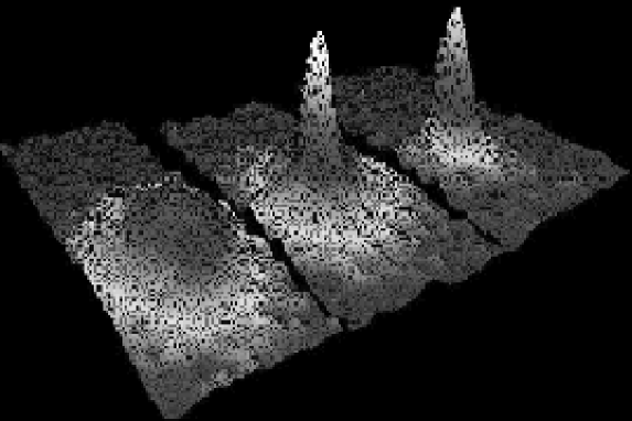
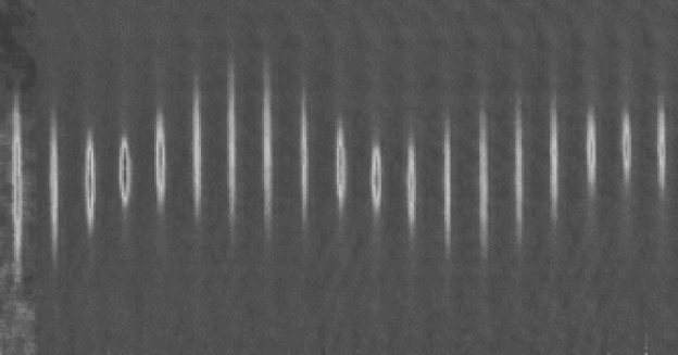
One of the most relevant features of these trapped Bose gases is that they are inhomogeneous and finite-sized systems, the number of atoms ranging typically from a few thousands to several millions. In most cases, the confining traps are well approximated by harmonic potentials. The trapping frequency, , provides also a characteristic length scale for the system, , of the order of a few microns in the available samples. Density variations occur on this scale. This is a major difference with respect to other systems, like for instance superfluid helium, where the effects of inhomogeneity take place on a microscopic scale fixed by the interatomic distance. In the case of 87Rb and 23Na, the size of the system is enlarged as an effect of repulsive two-body forces and the trapped gases can become almost macroscopic objects, directly measurable with optical methods. As an example, we show in Fig. 2 a sequence of “in situ” images of an oscillating condensate of sodium atoms taken at the Massachusetts Institute of Technology (MIT), where the mean axial extent is of the order of mm.
The fact that these gases are highly inhomogeneous has several important consequences. First BEC shows up not only in momentum space, as happens in superfluid helium, but also in co-ordinate space. This double possibility of investigating the effects of condensation is very interesting from both the theoretical and experimental viewpoints and provides novel methods of investigation for relevant quantities, like the temperature dependence of the condensate, energy and density distributions, interference phenomena, frequencies of collective excitations, and so on.
Another important consequence of the inhomogeneity of these systems is the role played by two-body interactions. This aspect will be extensively discussed in the present review. The main point is that, despite the very dilute nature of these gases (typically the average distance between atoms is more than ten times the range of interatomic forces), the combination of BEC and harmonic trapping greatly enhances the effects of the atom-atom interactions on important measurable quantities. For instance, the central density of the interacting gas at very low temperature can be easily one or two orders of magnitude smaller than the density predicted for an ideal gas in the same trap, as shown in Fig. 3. Despite the inhomogeneity of these systems, which makes the solution of the many-body problem nontrivial, the dilute nature of the gas allows one to describe the effects of the interaction in a rather fundamental way. In practice a single physical parameter, the -wave scattering length, is sufficient to obtain an accurate description.
The recent experimental achievements of BEC in alkali vapors have renewed a great interest in the theoretical studies of Bose gases. A rather massive amount of work has been done in the last couple of years, both to interpret the initial observations and to predict new phenomena. In the presence of harmonic confinement, the many-body theory of interacting Bose gases gives rise to several unexpected features. This opens new theoretical perspectives in this interdisciplinary field, where useful concepts coming from different areas of physics (atomic physics, quantum optics, statistical mechanics and condensed matter physics) are now merging together.
The natural starting point for studying the behavior of these systems is the theory of weakly interacting bosons which, for inhomogeneous systems, takes the form of the Gross-Pitaevskii theory. This is a mean-field approach for the order parameter associated with the condensate. It provides closed and relatively simple equations for describing the relevant phenomena associated with BEC. In particular, it reproduces typical properties exhibited by superfluid systems, like the propagation of collective excitations and the interference effects originating from the phase of the order parameter. The theory is well suited to describing most of the effects of two-body interactions in these dilute gases at zero temperature and can be naturally generalized to explore also thermal effects.
An extensive discussion of the application of mean-field theory to these systems is the main basis of the present review article. We also give, whenever possible, simple arguments based on scales of length, energy and density, in order to point out the relevant parameters for the description of the various phenomena.
There are several topics which are only marginally discussed in our paper. These include, among others, collisional and thermalization processes, phase diffusion phenomena, light scattering from the condensate and analogies with systems of coherent photons. In this sense our work is complementary to other recent review articles (Burnett, 1996; Parkins and Walls, 1998). Furthermore in our paper we do not discuss the physics of ultracold collisions and the determination of the scattering length which have been recently the object of important experimental and theoretical studies in the alkalis (Heinzen, 1997; Weiner et al., 1998).
The plan of the paper is the following:
In Sec. II we summarize the basic features of the noninteracting Bose gas in harmonic traps and we introduce the first relevant length and energy scales, like the oscillator length and the critical temperature. We also comment on finite size effects, on the role of dimensionality and on the possible relevance of anharmonic traps.
In Sec. III we discuss the effects of the interaction on the ground state. We develop the formalism of mean-field theory, based on the Gross-Pitaevskii equation. We consider the case of gases interacting with both repulsive and attractive forces. We then discuss in detail the large limit for systems interacting with repulsive forces, leading to the so called Thomas-Fermi approximation, where the ground state properties can be calculated in analytic form. In the last part, we discuss the validity of the mean-field approach and give explicit results for the first corrections, beyond mean-field, to the ground state properties, including the quantum depletion of the condensate, i.e., the decrease in the condensate fraction produced by the interaction.
In Sec. IV we investigate the dynamic behavior of the condensate using the time dependent Gross-Pitaevskii equation. The equations of motion for the density and the velocity field of the condensate in the large limit, where the Thomas-Fermi approximation is valid, are shown to have the form of the hydrodynamic equations of superfluids. We also discuss the dynamic behavior in the nonlinear regime (large amplitude oscillations and free expansion), the collective modes in the case of attractive forces and the transition from collective to single-particle states in the spectrum of excitations.
In Sec. V we discuss thermal effects. We show how one can define the thermodynamic limit in these inhomogeneous systems and how interactions modify the behavior compared to the noninteracting case. We extensively discuss the occurrence of scaling properties in the thermodynamic limit. We review several results for the shift of the critical temperature and for the temperature dependence of thermodynamic functions, like the condensate fraction, the chemical potential and the release energy. We also discuss the behavior of the excitations at finite temperature.
In Sec. VI we illustrate some features of these trapped Bose gases in connection with superfluidity and phase coherence. We discuss in particular the structure of quantized vortices and the behavior of the moment of inertia, as well as interference phenomena and quantum effects beyond mean-field theory, like the collapse-revival of collective oscillations.
In Sec. VII we draw our conclusions and we discuss some further future perspectives in the field.
The overlap between current theoretical and experimental investigations of BEC in trapped alkalis is already wide and rich. Various theoretical predictions, concerning the ground state, dynamics and thermodynamics are found to agree very well with observations; others are stimulating new experiments. The comparison between theory and experiments then represents an exciting feature of these novel systems, which will be frequently emphasized in the present review.
II The ideal Bose gas in a harmonic trap
A The condensate of noninteracting bosons
An important feature characterizing the available magnetic traps for alkali atoms is that the confining potential can be safely approximated with the quadratic form
| (1) |
Thus the investigation of these systems starts as a textbook application of nonrelativistic quantum mechanics for identical point-like particles in a harmonic potential.
The first step consists in neglecting the atom-atom interaction. In this case, almost all predictions are analytical and relatively simple. The many-body Hamiltonian is the sum of single-particle Hamiltonians whose eigenvalues have the form
| (2) |
where are non-negative integers. The ground state of noninteracting bosons confined by the potential (1) is obtained by putting all the particles in the lowest single-particle state (), namely , where is given by
| (3) |
and we have introduced the geometric average of the oscillator frequencies:
| (4) |
The density distribution then becomes and its value grows with . The size of the cloud is instead independent of and is fixed by the harmonic oscillator length
| (5) |
which corresponds to the average width of the Gaussian (3). This is the first important length scale of the system. In the available experiments, it is typically of the order of m. At finite temperature only part of the atoms occupy the lowest state, the others being thermally distributed in the excited states at higher energy. The radius of the thermal cloud is larger than . A rough estimate can be obtained by assuming and approximating the density of the thermal cloud with a classical Boltzmann distribution . If , the width of the Gaussian is , and hence larger than . The use of a Bose distribution function does not change significantly this estimate.
The above discussion reveals that Bose-Einstein condensation in harmonic traps shows up with the appearance of a sharp peak in the central region of the density distribution. An example is shown in Fig. 4, where we plot the prediction for the condensate and thermal densities of noninteracting particles in a spherical trap at a temperature , where is the temperature at which condensation occurs (see discussion in the next section). The curves correspond to the column density, namely the particle density integrated along one direction, ; this is a typical measured quantity, the direction being the direction of the light beam used to image the atomic cloud. By plotting directly the density , the ratio of the condensed and noncondensed densities at the center would be even larger.
By taking the Fourier transform of the ground state wave function, one can also calculate the momentum distribution of the atoms in the condensate. For the ideal gas, it is given by a Gaussian centered at zero momentum and having a width proportional to . The distribution of the thermal cloud is, also in momentum space, broader. Using a classical distribution function one finds that the width is proportional to . Actually, the momentum distributions of the condensed and noncondensed particles of an ideal gas in harmonic traps have exactly the same form as the density distributions and shown in Fig. 4.
The appearence of the condensate as a narrow peak in both co-ordinate and momentum space is a peculiar feature of trapped Bose gases having important consequences in both the experimental and theoretical analysis. This is different from the case of a uniform gas where the particles condense into a state of zero momentum, but BEC cannot be revealed in co-ordinate space, since the condensed and noncondensed particles fill the same volume.
Indeed, the condensate has been detected experimentally as the occurrence of a sharp peak over a broader distribution, in both the velocity and spatial distributions. In the first case, one lets the condensate expand freely, by switching-off the trap, and measures the density of the expanded cloud with light absorption (Anderson et al., 1995). If the particles do not interact, the expansion is ballistic and the imaged spatial distribution of the expanding cloud can be directly related to the initial momentum distribution. In the second case, one measures directly the density of the atoms in the trap by means of dispersive light scattering (Andrews et al., 1996). In both cases, the appearence of a sharp peak is the main signature of Bose-Einstein condensation. An important theoretical task consists of predicting how the shape of these peaks is modified by the inclusion of two-body interactions. As anticipated in Fig. 3, the interactions can change the picture drastically. This effect will be deeply discussed in Sec. III.
The shape of the confining field fixes also the symmetry of the problem. One can use spherical or axially symmetric traps, for instance. The first experiments on rubidium and sodium were carried out with axial symmetry. In this case one can define an axial co-ordinate and a radial co-ordinate and the corresponding frequencies, and . The ratio between the axial and radial frequencies, , fixes the asymmetry of the trap. For the trap is cigar-shaped while for is disk-shaped. In terms of the ground state (3) for noninteracting bosons can be rewritten as
| (6) |
Here is the harmonic oscillator length in the - plane and, since , one has also .
The choice of an axially symmetric trap has proven useful for providing further evidence of Bose-Einstein condensation from the analysis of the momentum distribution. To understand this point, let us take the Fourier transform of the wave function (6): . From this one can calculate the average axial and radial widths. Their ratio,
| (7) |
is fixed by the asymmetry parameter of the trap. Thus, the shape of the expanded cloud in the - plane is an ellipse, the ratio between the two axis (aspect ratio) being equal to . If the particles, instead of being in the lowest state (condensate), were thermally distributed among many eigenstates at higher energy, their distribution function would be isotropic in momentum space, according to the equipartition principle, and the aspect ratio would be equal to . Indeed, the occurrence of anisotropy in the condensate peak has been interpreted from the very beginning as an important signature of BEC (Anderson et al., 1995; Davis et al., 1995; Mewes et al., 1996a). In the case of the experiment at the Joint Institute for Laboratory Astrophysics (JILA) in Boulder, the trap is disk-shaped with . The first measured value of the aspect ratio was about % larger than the prediction, , of the noninteracting model (Anderson et al., 1995). Of course, a quantitative comparison can be obtained only including the atom-atom interaction, which affects the dynamics of the expansion (Holland and Cooper, 1996; Dalfovo and Stringari, 1996; Holland et al., 1997; Dalfovo et al., 1997c). However, the noninteracting model already points out this interesting effect due to anisotropy.
B Trapped bosons at finite temperature: thermodynamic limit
At temperature , the total number of particles is given, in the grand-canonical ensemble, by the sum
| (8) |
while the total energy is given by
| (9) |
where is the chemical potential and . Below a given temperature the population of the lowest state becomes macroscopic and this corresponds to the onset of Bose-Einstein condensation. The calculation of the critical temperature, the fraction of particles in the lowest state (condensate fraction) and the other thermodynamic quantities, starts from Eqs. (8) and (9) with the appropriate spectrum (de Groot, Hooman and Ten Seldam, 1950; Bagnato, Pritchard and Kleppner, 1987). Indeed the statistical mechanics of these trapped gases is less trivial than expected at first sight. Several interesting problems arise from the fact that these systems have a finite size and are inhomogeneous. For example, the usual definition of thermodynamic limit (increasing and volume with the average density kept constant) is not appropriate for trapped gases. Moreover the traps can be made very anisotropic, reaching the limit of quasi-2D and quasi-1D systems, so that interesting effects of reduced dimensionality can be also investigated.
As in the case of a uniform Bose gas, it is convenient to separate out the lowest eigenvalue from the sum (8) and call the number of particles in this state. This number can be macroscopic, i.e., of the order of , when the chemical potential becomes equal to the energy of the lowest state,
| (10) |
where is the arithmetic average of the trapping frequencies. Inserting this value in the rest of the sum, one can write
| (11) |
In order to evaluate this sum explicitly, one usually assumes that the level spacing becomes smaller and smaller when , so that the sum can be replaced by an integral:
| (12) |
This assumption corresponds to a semiclassical description of the excited states. Its validity implies that the relevant excitation energies, contributing to the sum (11), are much larger than the level spacing fixed by the oscillator frequencies. The accuracy of the semiclassical approximation (12) is expected to be good if the number of trapped atoms is large and . It can be tested a posteriori by comparing the integral (12) with the numerical summation (11).
The integral (12) can be easily calculated by changing variables (, etc.). One finds
| (13) |
where is the Riemann -function and is the geometric average (4). From this result one can also obtain the transition temperature for Bose-Einstein condensation. In fact, by imposing that at the transition, one gets
| (14) |
For temperatures higher than the chemical potential is less than and becomes -dependent, while the population of the lowest state is of the order of instead of . The proper thermodynamic limit for these systems is obtained by letting and , while keeping the product constant. With this definition the transition temperature (14) is well defined in the thermodynamic limit. Inserting the above expression for into Eq. (13) one gets the -dependence of the condensate fraction for :
| (15) |
The same result can be also obtained by rewriting (12) as an integral over the energy, in the form
| (16) |
where is the density of states. The latter can be calculated by using the spectrum (2) and turns out to be quadratic in : . Inserting this value into (16), one finds again result (13). The integral gives instead the total energy of the system (9) for which one finds the result
| (17) |
Starting from the energy one can calculate specific heat, entropy and the other thermodynamic quantities.
These results can be compared with the well known theory of uniform Bose gases (see, for example, Huang, 1987). In this case, the eigenstates of the Hamiltonian are plane waves of energy , with the density of states given by , where is the volume. The sum (8) gives and , with , while the energy is given by .
Another quantity of interest, which can be easily calculated using the semiclassical approximation, is the density of thermal particles . The sum of and the condensate density, , gives the total density . At and in the thermodynamic limit, the thermal density is given by the integral over momentum space , where is the semiclassical energy in phase space. The result is
| (18) |
where is the thermal wavelength. The function belongs to the class of functions [see, for example, Huang (1987)]. By integrating over space one gets again the number of thermally depleted atoms , consistently with Eq. (15). In a similar way one can obtain the distribution of thermal particles in momentum space: .
The above analysis points out the existence of two relevant scales of energy for the ideal gas: the transition temperature, , and the average level spacing, . From expression (14), one clearly sees that can be much larger than . In the available traps, with ranging from a few thousand to several millions, the transition temperature is 20 to 200 times larger than . This also means that the semiclassical approximation is expected to work well in these systems on a wide and useful range of temperatures. The frequency is fixed by the trapping potential and ranges typically from tens to hundreds of Hertz. This gives of the order of a few nK. In one of the first experiments at JILA (Ensher et al., 1996) for example, the average level spacing was about nK, corresponding to a critical temperature [see Eq. (14)] of about nK with atoms in the trap. We also note that, for the ideal gas, the chemical potential is of the same order of , as shown by Eq. (10). However, as we will see later on, its value depends significantly on the atom-atom interaction and shall consequently provide a third important scale of energy.
The noninteracting harmonic oscillator model has guided experimentalists to the proper value of the critical temperature. In fact, the measured transition temperature was found to be very close to the ideal gas value (14), the occupation of the condensate becoming macroscopically large below the critical temperature as predicted by (15). As an example, in Fig. 5 we show the first experimental results obtained at JILA (Ensher et al., 1996). The occurrence of a sudden transition at is evident. Similar results have been obtained also at MIT (Mewes et al., 1996a). Apart from problems related to temperature calibration, a more quantitative comparison between theory and experiments requires the inclusion of two main effects: the fact that these gases have a finite number of particles and that they are interacting. The role of interactions will be analysed extensively in the next sections. Here we briefly discuss the relevance of finite size corrections.
C Finite size effects
The number of atoms that can be put into the traps is not truly macroscopic. So far experiments have been carried out with a maximum of about atoms. As a consequence, the thermodynamic limit is never reached exactly. A first effect is the lack of discontinuities in the thermodynamic functions. Hence Bose-Einstein condensation in these trapped gases is not, strictly speaking, a phase transition. In practice, however, the macroscopic occupation of the lowest state occurs rather abruptly as temperature is lowered and can be observed, as clearly shown in Fig. 5. The transition is actually rounded with respect to the predictions of the limit, but this effect, though interesting, is small enough to make the words transition and critical temperature meaningful even for finite-sized systems. It is also worth noticing that, instead of being a limitation, the fact that is finite makes the system potentially richer, because new interesting regimes can be explored even in cases where there is no real phase transition in the thermodynamic limit. An example is BEC in 1D, as we will see in Sec. II D.
In order to work out the thermodynamics of a noninteracting Bose gas, all one needs is the spectrum of single particle levels entering the Bose distribution function. Working in the grand-canonical ensemble for instance, the average number of atoms is given by the sum (8) and it is not necessary to take the limit. In fact, the explicit summation can be carried out numerically (Ketterle and van Druten, 1996b) for a fixed number of particles and a given temperature, the chemical potential being a function of and . The condensate fraction , obtained in this way, turns out to be smaller than the thermodynamic limit prediction (15) and, as expected, the transition is rounded off. An example of an exact calculation of the condensate fraction for noninteracting particles is shown in Fig. 6 (circles). With their numerical calculation, Ketterle and van Druten (1996b) found that finite size effects are significant only for rather small values of , less than about . They calculated also the occupation of the first excited levels, finding that the fraction of atoms in these states vanishes for and is very small already for of the order of .
The first finite size correction to the law (15) for the condensate fraction can be evaluated analytically by studying the large limit of the sum (8) (Grossmann and Holthaus, 1995; Ketterle and van Druten, 1996b; Kirsten and Toms 1996; Haugerud, Haugset and Ravndal, 1997). The result for is given by
| (19) |
To the lowest order, finite size effects decrease as and depend on the ratio of the arithmetic () and geometric () averages of the oscillator frequencies. For axially symmetric traps this ratio depends on the deformation parameter as . For prediction (19) is already indistinguishable from the exact result obtained by summing explicitly over the excited states of the harmonic oscillator Hamiltonian, apart from a narrow region near where higher order corrections should be included to get the exact result. This is well illustrated in Fig. 6, where we plot the prediction (19) (solid line) together with the exact calculation obtained directly from (8) (circles). Both predictions are also compared with the thermodynamic limit, .
Finite size effects reduce the condensate fraction and thus result in a lowering of the transition temperature as compared to the limit. By setting the left hand side of Eq. (19) equal to zero one can estimate the shift of the critical temperature to order (Grossmann and Holthaus, 1995; Ketterle and van Druten, 1996b; Kirsten and Toms, 1996):
| (20) |
Another problem, which deserves to be mentioned in connection with the finite size of the system, is the equivalence between different statistical ensembles and the problem of fluctuations. In the thermodynamic limit the grand canonical, canonical and microcanonical ensembles are expected to provide the same results. However, their equivalence is no longer ensured when is finite. Rigorous results concerning the ideal Bose gas in a box and, in particular, the behavior of fluctuations, can be found in Ziff et al. (1977), and Angelescu et al. (1996). In the case of a trapped gas, Gajda and Rza̧żewski (1997) have shown that the differences between the predictions of the micro- and grand canonical ensembles for the temperature dependence of the condensate fraction are small already at . The fluctuations of the number of atoms in the condensate are instead much more sensitive to the choice of the ensemble (Navez et al., 1997; Wilkens and Weiss, 1997; see also Holthaus, Kalinowski and Kirsten, 1998, and references therein). Inclusion of two-body interactions can, however, change the scenario significantly (Giorgini, Pitaevskii and Stringari, 1998).
D Role of dimensionality
So far we have discussed the properties of the ideal Bose gas in three-dimensional space. Though the trapping frequencies in each direction can be quite different, nevertheless the relevant results for the temperature dependence of the condensate have been obtained assuming that is much larger than all the oscillator energies . In order to observe effects of reduced dimensionality, one should remove such a condition in one or two directions.
The statistical behavior of 2D and 1D Bose gases exhibits very peculiar features. Let us first recall that in a uniform gas Bose-Einstein condensation cannot occur in 2D and 1D at finite temperature because thermal fluctuations destabilize the condensate. This can be seen by noting that, for an ideal gas in the presence of BEC, the chemical potential vanishes and the momentum distribution, , exhibits an infrared divergence. In the thermodynamic limit, this yields a divergent contribution to the integral in 2D and 1D, thereby violating the normalization condition. The absence of BEC in 1D and 2D can be also proven for interacting uniform systems, as shown by Hohenberg (1967).
In the presence of harmonic trapping, the effects of thermal fluctuations are strongly quenched due to the different behavior exhibited by the density of states . In fact, while in the uniform gas behaves as , where is the dimensionality of space, in the presence of an harmonic potential one has instead the law and, consequently, the integral (16) converges also in 2D. The corresponding value of the critical temperature is given by
| (21) |
where (see, for example, Mullin, 1997, and references therein). One notes first that in 2D the thermodynamic limit corresponds to taking and with the product kept constant. In order to achieve 2D Bose-Einstein condensation in real 3D traps, one should choose the frequency in the third direction large enough to satisfy the condition ; this implies rather severe conditions on the deformation of the trap. The main features of BEC in 2D gases confined in harmonic traps and, in particular, the applicability of the Hohenberg theorem and of its extensions to nonuniform gases, have been discussed in details by Mullin (1997).
In 1D the situation is also very interesting. In this case, Bose-Einstein condensation cannot occur even in the presence of harmonic confinement because of the logarithmic divergence in the integral (16). This means that the critical temperature for 1D Bose-Einstein condensation tends to zero in the thermodynamic limit if one keeps the product fixed. In fact, in 1D the critical temperature for the ideal Bose gas can be estimated to be (Ketterle and van Druten, 1996b)
| (22) |
with . Despite the fact that one cannot have BEC in the thermodynamic limit, nevertheless for finite values of the system can exhibit a large occupation of the lowest single-particle state in a useful interval of temperatures. Furthermore, if the value of and the parameters of the trap are chosen in a proper way, one observes a new interesting phenomenon associated with the macroscopic occupation of the lowest energy state, taking place in two distinct steps (van Druten and Ketterle, 1997). This happens when the relevant parameters of the trap satisfy simultaneously the conditions and , where coincides with the usual critical temperature given in Eq. (14) and is the frequency of the trap in the - plane. In the interval , only the radial degrees of freedom are frozen, while no condensation occurs in the axial degrees of freedom. At lower temperatures, below , also the axial variables start being frozen and the overall ground state is occupied in a macroscopic way. An example of this two-step BEC is shown in Fig. 7. It is also interesting to notice that the conditions for the occurrence of two-step condensation in harmonic potentials are peculiar of the 1D geometry. In fact, it is easy to check that the corresponding conditions and , which would yield two-step BEC in 2D, cannot be easily satisfied because of the absence of the factor.
It is finally worth pointing out that the above discussion concerns the behavior of the ideal Bose gas. Effects of two-body interactions are expected to modify in a deep way the nature of the phase transition in reduced dimensionality. In particular, interacting Bose systems exhibit the well known Berezinsky-Kosterlitz-Thouless transition in 2D (Berezinsky, 1971; Kosterlitz and Thouless, 1973). The case of trapped gases in 2D has been recently discussed by Mullin (1998) and is expected to become an important issue in future investigations.
E Non harmonic traps and adiabatic transformations
A crucial step to reach the low temperatures needed for BEC in the experiments realized so far is evaporative cooling. This technique is intrinsically irreversible since it is based on the loss of hot particles from the trap. New interesting perspectives would open if one could adiabatically cool the system in a reversible way (Ketterle and Pritchard, 1992; Pinkse et al., 1997). Reversible cooling of the gas is achieved by adiabatically changing the shape of the trap at a rate slow compared to the internal equilibration rate.
An important class of trapping potentials for studying the effects of adiabatic changes is provided by power-law potentials of the form
| (23) |
where, for simplicity, we assume spherical symmetry. The critical temperature for Bose-Einstein condensation in the trap (23) has been calculated by Bagnato, Pritchard and Kleppner (1987) and is given by
| (24) |
Here we have introduced the parameter , while is the usual gamma function. By setting and , one recovers the result for the transition temperature in an isotropic harmonic trap. The result for a rigid box is instead obtained by letting .
It is straightforward to work out the thermodynamics of a noninteracting gas in the confining potential (23) (Bagnato, Pritchard and Kleppner, 1987; Pinkse et al. 1997). For example, for the condensate fraction one finds: . More relevant to the discussion of reversible processes is the entropy which remains constant during the adiabatic change. Above the system can be approximated by a classical Maxwell-Boltzmann gas and the entropy per particle takes the simple form
| (25) |
From this equation one sees that the entropy depends on the parameter of the external potential (23) only through the ratio . Thus, for a fixed power-law dependence of the trapping potential ( fixed), an adiabatic change of , like for example an adiabatic expansion of the harmonic trap, does not bring us closer to the transition, since the ratio remains constant. A reduction of the ratio is instead obtained by increasing adiabatically , that is, changing the power-law dependence of the trapping potential (Pinkse et al. 1997). For example, in going from a harmonic () to a linear trap (), one gets the relation between the initial and final reduced temperature . In this case a system at twice the critical temperature () can be cooled down to nearly the critical point (). Using this technique it should be possible, by a proper change of , to cool adiabatically the system from the high temperature phase without condensate down to temperatures below with a large fraction of atoms in the condensate state.
The possibility of reaching BEC using adiabatic transformations has been recently successfully explored in an experiment carried out at MIT (Stamper-Kurn et al., 1998b).
III Effects of interactions: ground state
A Order parameter and mean-field theory
The many body Hamiltonian describing interacting bosons confined by an external potential is given, in second quantization, by:
| (26) |
where and are the boson field operators that annihilate and create a particle at the position , respectively, and is the two-body interatomic potential.
The ground state of the system as well as its thermodynamic properties can be directly calculated starting from the Hamiltonian (26). For instance, Krauth (1996) has used a Path Integral Monte Carlo method to calculate the thermodynamic behavior of atoms interacting with a repulsive “hard-sphere” potential. In principle, this procedure gives exact results within statistical errors. However, the calculation can be heavy or even impracticable for systems with much larger values of . Mean-field approaches are commonly developed for interacting systems in order to overcome the problem of solving exactly the full many-body Schrödinger equation. Apart from the convenience of avoiding heavy numerical work, mean-field theories allow one to understand the behavior of a system in terms of a set of parameters having a clear physical meaning. This is particularly true in the case of trapped bosons. Actually most of the results reviewed in this paper show that the mean-field approach is very effective in providing quantitative predictions for the static, dynamic and thermodynamic properties of these trapped gases.
The basic idea for a mean-field description of a dilute Bose gas was formulated by Bogoliubov (1947). The key point consists in separating out the condensate contribution to the bosonic field operator. In general, the field operator can be written as , where are single-particle wave functions and are the corresponding annihilation operators. The bosonic creation and annihilation operators and are defined in Fock space through the relations
| (27) | |||||
| (28) |
where are the eigenvalues of the operator giving the number of atoms in the single-particle -state. They obey the usual commutation rules:
| (29) |
Bose-Einstein condensation occurs when the number of atoms of a particular single-particle state becomes very large: and the ratio remains finite in the thermodynamic limit . In this limit the states with and correspond to the same physical configuration and, consequently, the operators and can be treated like -numbers: . For a uniform gas in a volume , where BEC occurs in the single-particle state having zero momentum, this means that the field operator can be decomposed in the form . By treating the operator as a small perturbation, Bogoliubov developed the “first-order” theory for the excitations of interacting Bose gases.
The generalization of the Bogoliubov prescription to the case of nonuniform and time dependent configurations is given by
| (30) |
where we have used the Heisenberg representation for the field operators. Here is a complex function defined as the expectation value of the field operator: . Its modulus fixes the condensate density through . The function possesses also a well-defined phase and, similarly to the case of uniform gases, this corresponds to assuming the occurrence of a broken gauge symmetry in the many-body system.
The function is a classical field having the meaning of an order parameter and is often called “wave function of the condensate”. It characterizes the off-diagonal long-range behavior of the one-particle density matrix . In fact the decomposition (30) implies the following asymptotic behavior (Ginzburg and Landau, 1950; Penrose, 1951; Penrose and Onsager, 1956):
| (31) |
Notice that, strictly speaking, in a finite-sized system neither the concept of broken gauge symmetry, nor the one of off-diagonal long-range order can be applied. The condensate wave function has nevertheless still a clear meaning: it can be in fact determined through the diagonalization of the one-body density matrix, , and corresponds to the eigenfunction, , with the largest eigenvalue, . This procedure has been used, for example, to explore Bose-Einstein condensation in finite drops of liquid helium by Lewart et al. (1988). The connection between the condensate wave function, defined through the diagonalization of the density matrix and the concept of order parameter commonly used in the theory of superfluidity, is an interesting and nontrivial problem in itself. Another important question concerns the possible fragmentation of the condensate, taking place when two or more eigenstates of the density matrix are macroscopically occupied. One can show (Nozières and Saint James, 1982; Nozières, 1995) that, due to exchange effects, in uniform gases interacting with repulsive forces the fragmentation costs a macroscopic energy. The behavior can be however different in the presence of attractive forces and almost degenerate single-particle states (Nozières and Saint James, 1982; Kagan, Shlyapnikov and Walraven, 1996; Wilkin, Gunn and Smith, 1998).
The decomposition (30) becomes particularly useful if is small, i.e., when the depletion of the condensate is small. Then, an equation for the order parameter can be derived by expanding the theory to the lowest orders in as in the case of uniform gases. The main difference is that here one gets also a nontrivial “zeroth-order” theory for .
In order to derive the equation for the condensate wave function , one has to write the time evolution of the field operator using the Heisenberg equation with the many-body Hamiltonian (26):
| (32) | |||||
| (33) |
Then one has to replace the operator with the classical field . In the integral containing the atom-atom interaction , this replacement is, in general, a poor approximation when short distances are involved. In a dilute and cold gas, one can nevertheless obtain a proper expression for the interaction term by observing that, in this case, only binary collisions at low energy are relevant and these collisions are characterized by a single parameter, the -wave scattering length, independently of the details of the two-body potential. This allows one to replace in (33) with an effective interaction
| (34) |
where the coupling constant is related to the scattering length through
| (35) |
The use of the effective potential (34) in (33) is compatible with the replacement of with and yields the following closed equation for the order parameter:
| (36) |
This equation, known as Gross-Pitaevskii (GP) equation, was derived independently by Gross (1961 and 1963) and Pitaevskii (1961). Its validity is based on the condition that the -wave scattering length be much smaller than the average distance between atoms and that the number of atoms in the condensate be much larger than . The GP equation can be used, at low temperature, to explore the macroscopic behavior of the system, characterized by variations of the order parameter over distances larger than the mean distance between atoms.
The Gross-Pitaevskii equation (36) can also be obtained using a variational procedure:
| (37) |
where the energy functional is given by
| (38) |
The first term in the integral (38) is the kinetic energy of the condensate , the second is the harmonic oscillator energy , while the last one is the mean-field interaction energy . Notice that the mean-field term, , corresponds to the first correction in the virial expansion for the energy of the gas. In the case of non-negative and finite-range interatomic potentials, rigorous bounds for this term have been obtained by Dyson (1967) and Lieb and Yngvason (1998).
The dimensionless parameter controlling the validity of the dilute-gas approximation, required for the derivation of Eq. (36), is the number of particles in a “scattering volume” . This can be written as , where is the average density of the gas. Recent determinations of the scattering length for the atomic species used in the experiments on BEC give: nm for 23Na (Tiesinga et al., 1996), nm for 87Rb (Boesten et al., 1997) and nm for 7Li (Abraham et al., 1995). Typical values of density range instead from to cm-3, so that is always less than .
When the system is said to be dilute or weakly interacting. However, one should better clarify the meaning of the words “weakly interacting”, since the smallness of the parameter does not imply necessarily that the interaction effects are small. These effects, in fact, have to be compared with the kinetic energy of the atoms in the trap. A first estimate can be obtained by calculating the interaction energy, , on the ground state of the harmonic oscillator. This energy is given by , where the average density is of the order of , so that . On the other hand, the kinetic energy is of the order of and thus . One finally finds
| (39) |
This is the parameter expressing the importance of the atom-atom interaction compared to the kinetic energy. It can be easily larger than even if , so that also very dilute gases can exhibit an important nonideal behavior, as we will discuss in the following sections. In the first experiments with rubidium atoms at JILA (Anderson et al., 1995) the ratio was about , with of the order of a few thousands. Thus is larger than . In the experiments with 7Li at Rice University (Bradley et al., 1997; Sackett et al., 1997) the same parameter is smaller than , since the number of particles is of the order of and . Finally, in the experiments with sodium at MIT (Davis et al., 1995) the number of atoms in the condensate is very large () and .
Due to the assumption , the above formalism is strictly valid only in the limit of zero temperature, when all the particles are in the condensate. The dynamic behavior and the generalization to finite temperatures will be discussed in Secs. IV and V, respectively. Here we present the results for the stationary solution of the Gross-Pitaevskii (GP) equation at zero temperature.
B Ground state
For a system of noninteracting bosons in a harmonic trap, the condensate has the form of a Gaussian of average width [see Eq. (3)], and the central density is proportional to . If the atoms are interacting, the shape of the condensate can change significantly with respect to the Gaussian. The scattering length entering the Gross-Pitaevskii equation can be positive or negative, its sign and magnitude depending crucially on the details of the atom-atom potential. Positive and negative values of correspond to an effective repulsion and attraction between the atoms, respectively. The change can be dramatic when the interaction energy is much greater than the kinetic energy, that is, when . The central density is lowered (raised) by a repulsive (attractive) interaction and the radius of the atomic cloud consequently increases (decreases). This effect of the interaction has important consequences, not only for the structure of the ground state, but also for the dynamics and thermodynamics of the system, as we will see later on.
The ground state can be easily obtained within the formalism of mean-field theory. For this, one can write the condensate wave function as , where is the chemical potential and is real and normalized to the total number of particles, . Then the Gross-Pitaevskii equation (36) becomes
| (40) |
This has the form of a “nonlinear Schrödinger equation”, the nonlinearity coming from the mean-field term, proportional to the particle density . In the absence of interactions (), this equation reduces to the usual Schrödinger equation for the single-particle Hamiltonian and, for harmonic confinement, the ground state solution coincides, apart from a normalization factor, with the Gaussian function (3): . We note, in passing, that a similar nonlinear equation for the order parameter has been also considered in connection with the theory of superfluid helium near the -point (Ginzburg and Pitaevskii, 1958); in that case, however, the ingredients of the equation have a different physical meaning.
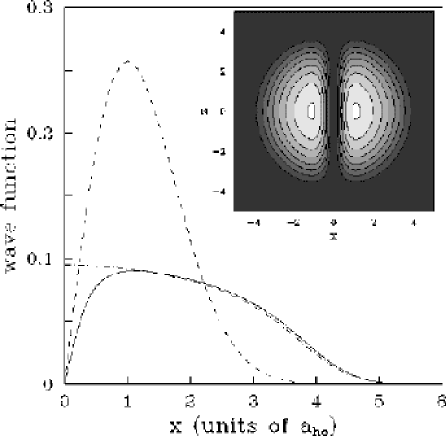
The numerical solution of the GP equation (40) is relatively easy to obtain (Edwards and Burnett, 1995; Ruprecht et al., 1995; Edwards et al., 1996b; Dalfovo and Stringari, 1996; Holland and Cooper, 1996). Typical wave functions , calculated from Eq. (40) with different values of the parameter , are shown in Figs. 8 and 9 for attractive and repulsive interaction, respectively. The effects of the interaction are revealed by the deviations from the Gaussian profile (3) predicted by the noninteracting model. Excellent agreement has been found by comparing the solution of the GP equation with the experimental density profiles obtained at low temperature (Hau et al., 1998), as shown in Fig. 3. The condensate wave function obtained with the stationary GP equation has been also compared with the results of an ab initio Monte Carlo simulation starting from Hamiltonian (26), finding a very good agreement (Krauth, 1996).
The role of the parameter , already discussed in the previous section, can be easily pointed out, in the Gross-Pitaevskii equation, by using rescaled dimensionless variables. Let us consider a spherical trap with frequency and use , and as units of length, density and energy, respectively. By putting a tilde over the rescaled quantities, Eq. (40) becomes
| (41) |
In these new units the order parameter satisfies the normalization condition . It is now evident that the importance of the atom-atom interaction is completely fixed by the parameter .
It is worth noticing that the solution of the stationary GP equation (40) minimizes the energy functional (38) for a fixed number of particles. Since the ground state has no currents, the energy is a functional of the density only, which can be written in the form
| (42) |
The first term corresponds to the quantum kinetic energy coming from the uncertainty principle; it is usually named “quantum pressure” and vanishes for uniform systems. In general, for a nonstationary order parameter, the kinetic energy in (38) includes also the contribution of currents in the form of an additional term containing the gradient of the phase of .
By direct integration of the GP equation (40) one finds the useful expression
| (43) |
for the chemical potential in terms of the different contributions to the energy functional (42). Further important relationships can be also found by means of the virial theorem. In fact, since the energy (38) is stationary for any variation of around the exact solution of the GP equation, one can choose scaling transformations of the form , and insert them in (38). By imposing the energy variation to vanish at first order in , one finally gets
| (44) |
where and . Analogous expressions are found by choosing similar scaling transformations for the and co-ordinates. By summing over the three directions one finally finds the virial relation:
| (45) |
The above results are exact within Gross-Pitaevskii theory and can be used, for instance, to check the numerical solutions of Eq. (40).
In a series of experiments the gas has been imaged after a sudden switching-off of the trap and the kinetic energy of the atoms has been measured by integrating over the observed velocity distribution. This energy, which is also called release energy, coincides with the sum of the kinetic and interaction energies of the atoms at the beginning of the expansion:
| (46) |
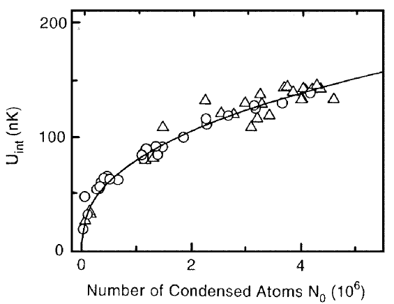
During the first phase of the expansion both the quantum kinetic energy (quantum pressure) and the interaction energy are rapidly converted into kinetic energy of motion. Then the atoms expand at constant velocity. Since energy is conserved during the expansion, its initial value (46), calculated with the stationary GP equation, can be directly compared with experiments. This comparison provides clean evidences for the crucial role played by two-body interactions. In fact, the noninteracting model predicts a release energy per particle given by , independent of . Conversely, the observed release energy per particle depends rather strongly on , in good agreement with the theoretical predictions for the interacting gas. In Figs. 10 and 11, we show the experimental data obtained at JILA (Holland et al.,1997) and MIT (Mewes et al., 1996a), respectively.
Finally, we notice that the balance between the quantum pressure and the interaction energy of the condensate fixes a typical length scale, called the healing length, . This is the minimum distance over which the order parameter can heal. If the condensate density grows from to within a distance , the two terms in Eq. (40) coming from the quantum pressure and the interaction energy are and , respectively. By equating them, one finds the following expression for the healing length:
| (47) |
This is a well known result for weakly interacting Bose gases. In the case of trapped bosons, one can use the central density, or the average density, to get an order of magnitude of the healing length. This quantity is relevant for superfluid effects. For instance, it provides the typical size of the core of quantized vortices (Gross, 1961; Pitaevskii, 1961). Note that in condensed matter physics the same quantity is often named “coherence length”, but the name “healing length” is preferable here in order to avoid confusion with different definitions of coherence length used in atomic physics and optics.
C Collapse for attractive forces
If forces are attractive (), the gas tends to increase its density in the center of the trap in order to lower the interaction energy, as seen in Fig. 8. This tendency is contrasted by the zero point kinetic energy which can stabilise the system. However, if the central density grows too much, the kinetic energy is no longer able to avoid the collapse of the gas. For a given atomic species in a given trap, the collapse is expected to occur when the number of particles in the condensate exceeds a critical value , of the order of . It is worth stressing that in a uniform gas, where quantum pressure is absent, the condensate is always unstable.
The critical number can be calculated at zero temperature by means of the Gross-Pitaevskii equation. The condensates shown in Fig. 8 are metastable, corresponding to local minima of the energy functional (38) for different . When increases, the depth of the local minimum decreases. Above the minimum no longer exists and the Gross-Pitaesvkii equation has no solution. For a spherical trap this happens at (Ruprecht et al., 1995)
| (48) |
For the axially symmetric trap with 7Li used in the experiments at Rice University (Bradley et al., 1995 and 1997; Sackett et al., 1997), the GP equation predicts (Dalfovo and Stringari, 1996; Dodd et al., 1996); this value is consistent with recent experimental measurements (Bradley et al., 1997; Sackett et al., 1997). The same problem has been investigated theoretically by several authors (Kagan, Shlyapnikov and Walraven, 1996; Houbiers and Stoof, 1996; Shuryak, 1996; Pitaevskii, 1996; Bergeman,1997).
A direct insight into the behavior of the gas with attractive forces can be obtained by means of a variational approach based on Gaussian functions (Baym and Pethick, 1996). For a spherical trap one can minimize the energy (38) using the ansatz
| (49) |
where is a dimensionless variational parameter which fixes the width of the condensate. One gets
| (50) |
This energy is plotted in Fig. 12 as a function of , for several values of the parameter . One clearly sees that the local minimum disappears when this parameter exceeds a critical value. This can be calculated by requiring that the first and second derivative of vanish at the critical point ( and ). One finds and . The last formula provides an estimate of the critical number of atoms, for given trap and atomic species, reasonably close to the value (48) obtained by solving exactly the GP equation. The Gaussian ansatz has been used by several authors in order to explore both static and dynamic properties of the trapped gases. The stability of a gas with has been explored in details, for instance, by Stoof (1997), Pérez-García et al. (1997), Shi and Zheng (1997a), Parola, Salasnich and Reatto (1998). The variational function proposed by Fetter (1997), which interpolates smoothly between the ideal gas and the Thomas-Fermi limit for positive , also reduces to a Gaussian for .
The behavior of the gas close to collapse could be significantly affected by mechanisms not included in the Gross-Pitaevskii theory. Among them, inelastic two- and three-body collisions can cause a loss of atoms from the condensate through, for instance, spin exchange or recombination (Hijmans et al., 1993; Edwards et al., 1996b; Moerdijk et al., 1996; Fedichev et al., 1996). This is an important problem not only for attractive forces but also for repulsive forces when the density of the system becomes large.
Recent discussions about the collapse, including quantum tunneling phenomena, can be found, for instance, in Sackett, Stoof and Hulet (1998), Kagan, Muryshev and Shlyapnikov (1998), Ueda and Leggett (1998), Ueda and Huang (1998).
D Large limit for repulsive forces
In the case of atoms with repulsive interaction (), the limit is particularly interesting, since this condition is well satisfied by the parameters , and used in most of current experiments. Moreover, in this limit the predictions of mean-field theory take a rather simple analytic form (Edwards and Burnett 1995; Baym and Pethick 1996).
As regards the ground state, the effect of increasing the parameter is clearly seen in Fig. 9: the atoms are pushed outwards, the central density becomes rather flat and the radius grows. As a consequence, the quantum pressure term in the Gross-Pitaevskii equation (40), proportional to , takes a significant contribution only near the boundary and becomes less and less important with respect to the interaction energy. If one neglects completely the quantum pressure in (40), one gets the density profile in the form
| (51) |
in the region where , and outside. This is often referred to as Thomas-Fermi (TF) approximation.
The normalization condition on provides the relation between chemical potential and number of particles:
| (52) |
Note that the chemical potential depends on the trapping frequencies, entering the potential given in (1), only through the geometric average [see Eq. (4)]. Moreover, since , the energy per particle turns out to be . This energy is the sum of the interaction and oscillator energies, since the kinetic energy gives a vanishing contribution for large . Finally, in the same limit, the release energy (46) coincides with the interaction energy: .
The chemical potential, as well as the interaction and oscillator energies obtained by solving numerically the GP equation (40) become closer and closer to the Thomas-Fermi values when increases (see for instance, Dalfovo and Stringari, 1996). For sodium atoms in the MIT traps, where is larger than , the Thomas-Fermi approximation is practically indistinguishable from the solution of the GP equation. The release energy per particle measured by Mewes et al. (1996a) is indeed well fitted with a law, as shown in Fig. 11. The same agreement is expected to occur for rubidium atoms in the most recent JILA traps, having larger than (Matthews et al., 1998).
The density profile (51) has the form of an inverted parabola, which vanishes at the classical turning point defined by the condition . For a spherical trap, this implies and, using result (52) for , one finds the following expression for the radius of the condensate
| (53) |
which grows with . For an axially symmetric trap, the widths in the radial and axial directions are fixed by the conditions . It is worth mentioning that, in the case of the cigar-shaped trap used at MIT, with a condensate of about sodium atoms, the axial width becomes macroscopically large ( mm), allowing for direct in situ measurements.
The value of the density (51) in the center of the trap is . It is worth stressing that this density is much lower than the one predicted for noninteracting particles. In the latter case, using Eq. (3) one gets . The ratio between the central densities in the two cases is then
| (54) |
and decreases with . For the available traps with 23Na and 87Rb, where ranges from about to , the atom-atom repulsion reduces the density by one or two orders of magnitude, which is a quite remarkable effect for such a dilute systems. An example was already shown in Fig. 3; in that case, the number of particles is about and .
In Fig. 13a we show the density profile for a gas in a spherical trap with . The comparison with the exact solution of the GP equation (40) shows that the TF approximation is very accurate except in the surface region close to . In part of the same figure, we plot the column density, , which is the measured quantity when the atomic cloud is imaged by light absorption or dispersive light scattering. Using the TF density (51) with , one finds . One notes that the accuracy of the Thomas-Fermi approximation is even better in the case of the column density, because the extra integration makes the cusp in the outer part of the condensate smoother.
The only region where the Thomas-Fermi density (51) is inadequate is close to the classical turning point. This region plays a crucial role for the calculation of the kinetic energy of the condensate. The shape of the outer part of the condensate is fixed by the balance of the zero point kinetic energy and the external potential. In particular, this balance can be used to define an effective surface thickness, . For a spherical trap, for instance, one can assume the two energies to have the form and , respectively. One then gets (Baym and Pethick, 1996)
| (55) |
this ratio is small when TF approximation is valid, i.e., when . It is interesting to compare the surface thickness with the healing length (47). In terms of the ratio one can write , showing that the healing length decreases with more rapidly than the surface thickness .
A good approximation for the density in the region close to the classical turning point, can be obtained by a suitable expansion of the GP equation (40). In fact, when , the trapping potential can be replaced with a linear ramp, , and the GP equation takes a universal form (Dalfovo, Pitaevskii and Stringari, 1996; Lundh, Pethick and Smith, 1997), yielding the rounding of the surface profile.
Using the above procedure it is possible to calculate the kinetic energy which, in the case of a spherical trap, is found to follow the asymptotic law
| (56) |
where is a numerical factor. Analogous expansions can be derived for the harmonic potential energy, , and interaction energy, , in the same large limit (Fetter and Feder, 1997). A straightforward derivation is obtained by using nontrivial relationships among the various energy components , and of Eq. (42). A first relation is given by the virial theorem (45). A second one is obtained by using expression (43) for the chemical potential and the thermodynamic definition . These two relationships, together with the asymptotic law (56) for the kinetic energy, allow one to obtain the expansions and . From them one gets the useful results
| (57) |
and
| (58) |
for the chemical potential and the total energy, respectively. In these equations and are the Thomas-Fermi values (52) and (53) of the chemical potential and the radius of the condensate. Equations (56)-(58), which apply to spherical traps, clearly show that the relevant small parameter in the large expansion is .
The Thomas-Fermi approximation (51) for the ground state density of trapped Bose gases is very useful not only for determining the static properties of the system, but also for dynamics and thermodynamics, as we will see in Secs. IV and V. It is worth noticing that this approximation can be derived more directly using local density theory as we are going to discuss in the next section.
E Beyond mean-field theory
Before closing this discussion about the effect of interactions on the ground state properties, we wish to come back to the basic question of the validity of the Gross-Pitaevskii theory. All the results so far presented are expected to be valid if the system is dilute, that is, if . In order to estimate the accuracy of this approach we will now calculate the first corrections to the mean-field approximation. Such corrections have been recently investigated in several papers as, for instance, by Timmermans, Tommasini and Huang (1997) and by Braaten and Nieto (1997). Here we limit the discussion to the case of repulsive interactions and large , where analytic results can be found. In fact, in this limit the solution of the stationary GP equation (40) for the ground state density can be safely replaced with the Thomas-Fermi expression (51) and the energy of the system is given by , where is the TF chemical potential (52).
Let us first discuss the behavior of the ground state density. For large one can use the local density approximation for the chemical potential:
| (59) |
The use of the local density approximation for is well justified in the thermodynamic limit , where the profile of the density distribution is very smooth. Equation (59) fixes the density profile of the ground state once the thermodynamic relation for the uniform fluid is known, the parameter in the l.h.s. of Eq. (59) being fixed by the normalization of the density. For example, in a very dilute Bose gas at , one has and immediately finds the mean-field Thomas-Fermi result (51). The first correction to the Bogoliubov equation of state is given by the law (Lee and Yang, 1957; Lee, Huang and Yang, 1957)
| (60) |
which includes nontrivial effects associated with the renormalization of the scattering length. Using expression (60) for , one can solve equation (59) by iteration. The result is
| (61) |
with given by
| (62) |
Then the energy can be also evaluated through the thermodynamic relation , and one finds
| (63) |
where, in the second term, we have safely used the lowest order relation . In an equivalent way, results (61)-(63) can be derived using a variational procedure by writing the energy functional of the system in the local density approximation.
Equations (62)-(63) show that, as expected, the corrections to the mean-field results are fixed by the gas parameter evaluated at the center of the trap. This quantity can be directly expressed in terms of the relevant parameters of the system:
| (64) |
Inserting typical values for the available experiments, the corrections to the chemical potential and the energy turn out to be of the order of %. These corrections to the mean-field predictions should be compared with the ones due to finite size effects (quantum pressure) in the solution of the Gross-Pitaevskii equation [see Eqs. (57) and (58)], which have a different dependence on the parameters and . One finds that finite size effects become smaller than the corrections given by Eqs. (62)-(63) when is larger than about .
Another important quantity to discuss is the quantum depletion of the condensate. This gives the fraction of atoms which do not occupy the condensate at zero temperature, because of correlation effects. The quantum depletion is ignored in the derivation of the Gross-Pitaevskii equation. It is consequently useful to have a reliable estimate of its value in order to check the validity of the theory. Also in this case we can use local density approximation (Timmermans, Tommasini and Huang, 1997) and write the density of atoms out of the condensate, , using Bogoliubov’s theory for uniform gases at density (see for example Huang, 1987). One gets . Integration of yields the result:
| (65) |
for the quantum depletion of the condensate. Similarly to the correction to the mean-field energy (63), this effect is very small (less than 1%) in the presently available experimental conditions.
The above results justify a posteriori the use of the Bogoliubov prescription for the Bose field operators and the perturbative treatment of the noncondensed part at zero temperature. We recall that this situation is completely different from the one of superfluid 4He where quantum depletion amounts to about 90% (Griffin, 1993; Sokol, 1995).
IV Effects of interactions: dynamics
A Excitations of the condensate and time dependent GP equation
The study of elementary excitations is a task of primary importance of quantum many-body theories. In the case of Bose fluids, in particular, it plays a crucial role in the understanding of the properties of superfluid liquid helium and was the subject of pioneering work by Landau, Bogoliubov and Feynman (for a recent discussion on the dynamic behavior of interacting Bose superfluids see, for instance, Griffin, 1993).
After the experimental realization of BEC in trapped Bose gases, there has been an intensive study of the excitations in these systems. Measurements of the frequency of the lowest modes have soon become available and the direct observation of the propagation of wave packets has been also obtained. In the meanwhile, on the theoretical side, a variety of papers has been written to explore several interesting features exhibited by the dynamic behavior of trapped Bose gases.
Let us start our discussion recalling that for dilute Bose gases an appropriate description of the excitations can be obtained from the time dependent GP equation (36) for the order parameter. This equation has been already used in Sec. III for evaluating the stationary solution characterizing the ground state. In the low temperature limit, where the properties of the excitations do not depend on temperature, the excited states can be found from the “classical” frequencies of the linearized GP equation. Namely, one can look for solutions of the form
| (66) |
corresponding to small oscillations of the order parameter around the ground state value. By keeping terms linear in the complex functions and , Eq. (36) becomes
| (67) | |||||
| (68) |
where . These coupled equations allow one to calculate the eigenfrequencies and hence the energies of the excitations. This formalism was introduced by Pitaevskii (1961), in order to investigate the excitations of vortex lines in a uniform Bose gas.
This procedure is also equivalent to the diagonalization of the Hamiltonian in Bogoliubov approximation, in which one expresses the field operator in terms of the quasiparticle operators and through (Fetter, 1972 and 1996)
| (69) |
By imposing the Bose commutation rules to the operators and , one finds that the quasiparticle amplitudes and must obey the normalization condition
| (70) |
In a uniform gas, the amplitudes and are plane waves and the resulting dispersion law takes the most famous Bogoliubov form (Bogoliubov, 1947)
| (71) |
where is the wavevector of the excitation and is the density of the gas. For large momenta the spectrum coincides with the free-particle energy . At low momenta Eq. (71) instead yields the phonon dispersion , where
| (72) |
is the sound velocity. It is worth noticing that this velocity coincides with the hydrodynamic expression for a gas with equation of state [see also the discussion after Eq. (79)].
In the case of harmonic trapping, an important role is played by the ratio , and one expects different behaviors in the two opposite limits and . In the first case, one recovers the excitation spectrum of the noninteracting harmonic potential [see Eq. (2)]. In the second case, one obtains a different dispersion law for the excitations of the system which are the analog of phonons [see Eq. (81) below].
The coupled equations (67)-(68) were first used to calculate numerically the excitations of trapped gases by Burnett and co-workers (Ruprecht et al., 1996; Edwards et al, 1996a and 1996c). Similar calculations have been also performed by other authors, for both spherical and anisotropic configurations (Singh and Rokhsar, 1996; Esry, 1997; Hutchinson, Zaremba and Griffin, 1997; Hutchinson and Zaremba, 1997; You, Hoston and Lewenstein,1997; Dalfovo et al., 1997a).
For spherical traps, the solutions of Eqs. (67)-(68) are characterized by the quantum numbers , and , where is the number of radial nodes, is the angular momentum of the excitation and its component. For axially symmetric traps the third component of angular momentum is still a good quantum number. In Fig. 14 we report the lowest solutions of even parity with and , obtained for a gas of rubidium atoms confined in an axially symmetric trap (). The asymmetry parameter of the trap () corresponds to the experimental conditions of Jin et al. (1996) and values of up to are considered. Actually the results are reported as a function of the dimensionless parameter where . The theoretical predictions are compared with the experimental results. In the experiments these oscillations are observed by shaking the condensate through the modulation of the trapping magnetic fields. The general agreement between theory and experiments is good and reveals the important role played by two-body interactions. In fact, in the absence of interactions, the eigenfrequencies would be the ones predicted by the ideal harmonic oscillator, which gives for both modes.
Among the various excitations exhibited by these trapped gases, special attention should be devoted to the dipole mode. This oscillation corresponds to the motion of the center of mass of the system which, due to the harmonic confinement, oscillates with the frequency of the harmonic trap (this frequency can of course be different in the three directions). Two-body interactions cannot affect this mode because, in the presence of harmonic trapping, the motion of the center of mass is exactly decoupled from the internal degrees of freedom of the system. This is best understood by considering Eq. (36) and looking for solutions of the form
| (73) |
where, for simplicity, we have considered only oscillations along the -axis. By a proper change of variables, , one finds that (73) corresponds to an exact solution of the time dependent equation (36) oscillating with frequency . This property holds not only in the context of the Gross-Pitaevskii equation, but is valid for any interacting system confined in a harmonic potential at zero as well as finite temperature, and is independent of statistics (Fermi or Bose). For example, such a decoupling is a well known property of shell model theory in nuclear physics (Elliott and Skyrme, 1955; Brink, 1957). It also exhibits interesting analogies with Kohn’s theorem for electrons in a static magnetic field, stating that the cyclotron frequency is not affected by interactions (Kohn, 1961) [see also Dobson (1994) and references therein for discussions about the generalization of Kohn’s theorem to the case of electrons confined in harmonic traps].
The fact that the dipole frequency is not affected by two-body interactions offers a direct test on the numerical accuracy of the various methods used to solve the equations of motion. On the other hand the experimental determination of the dipole frequency turns out to be a very useful procedure to check the harmonicity of the trap and to determine accurately the value of the trapping frequencies. The properties of the dipole excitation in the framework of Bogoliubov theory have been discussed in detail by Fetter and Rokhsar (1998) [see also Kimura and Ueda (1998)].
Of course the coupled equations (67)-(68) provide a full series of solutions, with different values of the corresponding quantum numbers. So far experiments have provided direct information only on the low energy modes which can be directly excited by suitable modulation of the harmonic trap. These excitations will be further discussed in the next section using the formalism of collisionless hydrodynamic equations. States at higher energy and multipolarity are also important, since they characterize the thermodynamic behavior of the system, as we will see later on.
Finally, we note that, starting from the solutions of Eqs. (67)-(68), one can also evaluate the density of particles out of the condensate at zero temperature (quantum depletion) by summing the square modulus of the “hole” amplitude over all the excited states: (Fetter, 1972). The results (Hutchinson, Zaremba and Griffin, 1997; Dalfovo et al., 1997a) are in agreement with the local density estimate (65).
B Large limit and collisionless hydrodynamics
When the number of atoms in the trap increases, the eigenfrequencies of the coupled equations (67)-(68) approach an asymptotic value. The new regime is achieved when the condition is satisfied. In this limit the excitations are properly described by the hydrodynamic theory of superfluids in the collisionless regime at zero temperature. In a dilute gas this theory can be explicitly derived starting from the time dependent GP equation (36). To this purpose, it is convenient to write the complex order parameter in terms of a modulus and a phase, as follows:
| (74) |
The phase fixes the velocity field
| (75) |
so that
| (76) |
The GP equation (36) can hence be rewritten in the form of two coupled equations for the density and the velocity field:
| (77) |
and
| (78) |
Equation (77) is the equation of continuity, while (78) establishes the irrotational nature of the superfluid motion. It is worth noticing that, at this stage, Eqs. (77) and (78) do not involve any approximation with respect to the GP equation (36) and can be used in the linear as well as nonlinear regimes.
If the repulsive interaction among atoms is strong enough, then the density profiles become smooth and one can safely neglect the kinetic pressure term, proportional to , in the equation for the velocity field, which then takes the form
| (79) |
This result corresponds to the equation of potential flow for a fluid whose pressure and density are related by the equation of state . Equations (77) and (79) have the typical structure of the dynamic equations of superfluids at zero temperature (see, for example, Pines and Nozieres, 1966, Vol.II) and can be viewed as a particular case of the more general Landau’s theory of superfluidity. According to this theory, which is valid if the relevant physical quantities change slowly on distances larger than the healing length, a complete description of the dynamics of the fluid is obtained by coupling the equation for the superfluid velocity field with a Boltzmann-type equation for the distribution function of elementary excitations [see, Lifshitz and Pitaevskii, 1981, §77]. At high temperature, when the mean free path of elementary excitations is short, one gets a system of two-fluid hydrodynamics equations. Conversely, at low temperature, where the role of thermally excited states is negligible, the same equations reduce to the hydrodynamic-type equations (77) and (79) involving only the superfluid velocity. In this sense, equations can be referred to as the hydrodynamic equations of superfluids. They should not be confused with the hydrodynamic equations valid in the collisional regime at high temperature.
The stationary solution of Eq. (79) coincides with the Thomas-Fermi density (51) while the time dependent equations (77) and (79), after linearization, take the following simplified form:
| (80) |
where , the quantity having the meaning of a local sound velocity.
The validity of the equation (80) is based on the assumption that the spatial variations of the density are smooth not only in the ground state, but also during the oscillation. In a uniform system () this is equivalent to imposing that the collective frequencies be much smaller than the chemical potential. In this case, the solutions of (80) are sound waves propagating with the Bogoliubov velocity (72). Sound waves can propagate also in nonuniform media, provided we look for solutions varying rapidly with respect to the size of the system, so that one can assume a locally uniform sound velocity (Landau and Lifshitz, 1987, §67). This is possible if both the conditions and are satisfied, where is the size of the condensate and is the wavevector of the sound wave. Furthermore, if the system is highly deformed and cigar-shaped, one can simultaneously satisfy the conditions and , characterizing one-dimensional waves propagating in the direction. Here and are the radii of the condensate in the axial and radial directions, respectively. In this case, one can show (Zaremba, 1998) that the sound velocity in the central region of the trap is given by , instead of the usual Bogoliubov value , where and is the value of the central density. The occurrence of the extra factor follows from the fact that, in the “one-dimensional” geometry, the sound velocity is fixed by the density averaged over the radial direction, which is of course smaller than its central value.
In the experiments of Andrews, Kurn et al. (1997), one-dimensional sound waves are generated by focusing a laser pulse in the center of the trap. A wave packet forms in this way, propagating outwards. It is then imaged at different times so that the value of the sound velocity can be directly measured. In Fig. 15 we show the observed values of at different densities. The agreement with the theoretical predictions is reasonably good especially at high density. Possible sources of inaccuracy at low density are discussed by the same authors. The theoretical analysis of the propagation of wave packets and sound waves in the elongated geometry has been the object of several recent works (Zaremba, 1998; Kavoulakis and Pethick, 1998; Stringari, 1998).
In these nonuniform condensates, as already said, oscillations having wavelength much smaller than the size of the system or, equivalently, frequency much larger than the trapping frequency , propagate as usual sound waves. Conversely, solutions of (80) at lower frequency, of the order of , involve a motion of the whole system (Baym and Pethick, 1996). They coincide with the low energy solutions of Eqs. (67)-(68) discussed in the previous section. For a spherical trap these solutions are defined in the interval and have the form where are polynomials of degree , containing only even powers. The dispersion law of the discretized normal modes is given by the formula (Stringari, 1996b)
| (81) |
This result can be compared with the prediction for noninteracting particles in harmonic potential:
| (82) |
with [see Eq. (2)]. Of particular interest is the case of the so called surface excitations () for which Eq. (81) predicts the dispersion law . The frequency of these modes is systematically smaller than the harmonic oscillator result . Notice that in the dipole case () the prediction (81) coincides with the oscillator frequency, in agreement with the general considerations discussed in the previous section.
As concerns compressional modes (), the lowest solution of (80) is the monopole oscillation, also called the breathing mode, characterized by the quantum numbers and . The formula (81) gives the result , higher than the corresponding prediction of the noninteracting model, which gives .
For a fixed value of the accuracy of prediction (81) is expected to become lower and lower as and increase. In fact, for large and the oscillations of the density have shorter wavelength and neglecting the kinetic energy pressure in (78) is no longer justified. In analogy with the case of uniform Bose gases, the condition for the applicability of the hydrodynamic theory of superfluids is expected to be . However, as discussed in Sec. IV E, more severe restrictions are imposed when one considers surface excitations.
The result (81) reveals that, in the Thomas-Fermi limit , the dispersion relation of the normal modes of the condensate has changed significantly from the noninteracting behavior, as a consequence of two-body interactions. However it might appear surprising that in this limit the dispersion does not depend any more on the value of the interaction parameter . This differs from the uniform case where the dispersion law, in the corresponding phonon regime, is given by and depends explicitly on the interaction through the velocity of sound. The behavior exibited in the harmonic trap is well understood if one notes that the values of are fixed by the boundary and vary as where is the size of the system. While in the box this size is fixed, in the case of harmonic confinement it increases with due to the repulsive effect of two-body interactions: . On the other hand the value of the sound velocity, calculated at the center of the trap, is given by and also increases with . One finally finds that in the product both the interaction parameter and the number of atoms in the trap cancel out, so that the collective frequency is proportional to the oscillator frequency .
The results for the spherical trap can be generalized to the case of anisotropic configurations. Let us consider the case of a harmonic oscillator trap with axial symmetry along the axis. In this case the differential equation (80) takes the form
| (83) |
where we have used . [We notice, in passing, that the corresponding Eq. (21) in Stringari (1996b) was misprinted, since it contains the chemical potential counted twice.]
Because of the axial symmetry of the trap the third component of the angular momentum is a good quantum number. However, in contrast to the spherical case, the dispersion law depends on . Explicit results are available in some particular cases. For example, quadrupole solutions of the form satisfy Eq. (83) for and . The resulting dispersion laws are:
| (84) |
and
| (85) |
Conversely the mode is coupled to the monopole excitation and the dispersion law of the two decoupled modes is given by (Stringari, 1996b)
| (86) |
When one recovers the solutions for the quadrupole and monopole excitations in the spherical trap. The occurrence of analytic solutions for the excitation spectrum, like Eqs. (81) and (83)-(86), is the result of nontrivial underlying symmetries of the Hamiltonian that have been exploited by Fliesser et al. (1997). The result (86) can be generalized to a triaxially deformed trap of the form (1). In this case, the collective frequencies are given by the solution of the equation
| (87) |
From Fig. 14 one can see that the experiments at JILA do not fully fall in the asymptotic regime, where the frequencies are given by Eqs. (84-86). Conversely the experimental results obtained on sodium vapors at MIT (Stamper-Kurn et al., 1998c) represent a very clear example of excitations belonging to the Thomas-Fermi regime. In this experiment the magnetic trap is highly asymmetric, with (cigar-shaped geometry). Furthermore the number of atoms is very high, so that the condition is well satisfied and the energies of the collective oscillations along the axial direction are much smaller than the chemical potential, . This explains the excellent agreement between the observed frequency for the lowest axial mode of even parity () and the theoretical prediction () given by Eq. (86) with . In Fig. 16 we show the oscillations observed in the MIT experiment (see also Fig. 2). These measurements correspond to nondestructive in situ images of the oscillating condensate, while the ones at JILA (Jin et al., 1996 and 1997), as well as the first experiments carried out at MIT (Mewes et al., 1996b) were taken after switching-off the trap and letting the gas expand.
For highly deformed traps it is possible to obtain simple analytic results also for the excitations with higher quantum numbers. For example, in the case of cigar-shaped traps () one finds the dispersion law (Fliesser et al., 1997; Stringari, 1998)
| (88) |
where is the relevant quantum number characterizing the spatial shape of the density oscillation . Equation (88) is valid if . It includes, as special cases, the dipole ( and “quadrupole” () modes already discussed. It also permits one to understand the transition between the discretized (small ) and “continuum” () regimes, through the identification where is the wave vector of “one-dimensional” phonons propagating with sound velocity . As already discussed, these phonons can be considered one-dimensional only if the conditions and are satisfied. The first condition implies large values of , the second one is equivalent to imposing .
Analogously for disk-shaped traps () the dispersion law of the lowest modes takes the analytic form (Stringari, 1998)
| (89) |
where is the number of radial nodes and is the -component of the angular momentum.
C Sum rules and collective excitations
In the previous section we have discussed the excitations of the condensate when atoms interact with repulsive forces (). In the opposite case of attractive interactions (), one expects a different behavior. For example, interesting effects can originate from the fact that the system becomes more and more compressible when approaching the critical number, , for collapse. In terms of the excitation spectrum, this means a lowering of the frequency of the monopole oscillation. For repulsive forces, we have previously discussed the Thomas-Fermi limit, in which the time dependent GP equation takes the form of the zero temperature hydrodynamic theory of superfluids. When the interaction is attractive, the large limit is never reached, since the collapse occurs at of the order of , and one has to solve numerically the GP equation (see, for example, Dodd et al., 1996) or use different theoretical schemes, as shown in the following.
A useful physical insight on the behavior of collective oscillations for both positive and negative can be obtained using the formalism of linear response and sum rules [see, for instance, Bohigas, Lane and Martorell (1979), Lipparini and Stringari (1989)]. This approach allows one to evaluate the energy weighted moments, , of the strength distribution function (dynamic form factor) associated with a given operator :
| (90) |
where the quantity is the excitation energy of the eigenstate of the Hamiltonian. Consequently, the method provides information on the dynamic behavior of the system. Quantities like or correspond to rigorous upper bounds for the energy of the lowest state excited by the operator . They are close to the exact energy when this state is highly collective, that is, when the strength distribution is almost exhausted by a single mode. This is often true in the case of trapped gases, as we will see below.
A major advantage of sum rules is that they can be often evaluated in a direct way, avoiding the full solution of the Schrödinger equation for the eigenstates of the Hamiltonian. For example, using the completeness of the eigenstates , the energy weighted moment, , can be easily transformed into the calculation of commutators involving the operator and the Hamiltonian:
| (91) |
Furthermore, if the operator depends only on spatial co-ordinates then only the kinetic energy gives a contribution to , whose calculation becomes straightforward. In a similar way, one can write the cubic energy weighted moment, , in the form . Unlike and , the inverse energy weighted moment, , cannot be expressed in terms of commutators; it can be however written in the useful form
| (92) |
where is the linear static response of the system.
Let us first consider the case of compressional modes. The natural monopole operator is given by the choice and, from (91), one gets the result for the energy weighted sum rule. Furthermore, in the monopole case one can easily evaluate also the inverse energy weighted sum rule through Eq. (92). In fact, the static response (monopole compressibility) is fixed by the linear change of the mean square radius induced by the external field . Adding this field to the Hamiltonian is equivalent to renormalizing the trapping harmonic potential and hence, for isotropic confinement, one can write
| (93) |
where is the frequency of the harmonic oscillator. Using the properties of the Gross-Pitaevskii equation (36), one can express exactly the derivative in terms of the square radius, , and its derivative with respect to . One finds (Zambelli, 1998)
| (94) |
where the term depending on the derivative arises from two-body interactions; in the case of an ideal gas, this term vanishes and the mean square radius, , is independent of .
Using the moments and one can define an average excitation energy, , through the ratio
| (95) |
yielding the useful result (Zambelli, 1998)
| (96) |
In the noninteracting case, one recovers . When is large and positive, the Thomas-Fermi approximation (51) for the density provides the analytic behavior of the radius, , and hence the result already discussed in the previous section. For negative and close to the critical size , the monopole frequency goes to zero because the compressibility of the system becomes larger and larger. Actually the -dependence of near can be determined analytically. For example, using the Gaussian variational procedure developed in Sec. III C, one finds the result , where is the square radius of the condensate at the critical value . As a consequence of this peculiar dependence, the monopole compressibility diverges near and the monopole frequency vanishes as (Singh and Rokhsar, 1996; Zambelli, 1998; Ueda and Leggett, 1998)
| (97) |
By using the numerical solution of the Gross-Pitaevskii equation to calculate the -dependence of the square radius one finds a slightly smaller value for the numerical coefficient in (97), namely instead of . It has been suggested that the behavior of the monopole frequency near might play an important role in the decay mechanism of the condensate for very close to , due to quantum tunneling (Ueda and Leggett, 1998).
In Fig. 17 we show the frequency obtained from Eq. (96) as a function of the parameter (solid line). The square radius has been calculated by solving numerically the stationary GP equation (40) in a spherical trap. As already said, the ratio (95) between moments of the strength distribution function provides a rigorous upper bound to the lowest monopole frequency. The comparison with the numerical solutions of the time dependent GP equation (circles) shows that the sum rule estimate actually gives an excellent approximation to the collective frequency for both positive and negative values of , practically indistinguishable from the exact result. This means that the strength distribution of the monopole operator almost coincides with a -function located at the energy of the lowest compressional mode. For the same reason, also the ratio turns out to be very close to (Zambelli, 1998).
Unlike the monopole frequency, the quadrupole frequency increases with when , due to the increase of the kinetic energy of the condensate. This behavior is well understood by calculating the quadrupole frequency through the ratio , where and are the energy and cubic energy weighted moments for the natural quadrupole operator . By explicitly working out the commutators of the two sum rules one finds the following result for the quadrupole frequency (Stringari, 1996b):
| (98) |
In the noninteracting gas one has and (98) gives the harmonic oscillator result . In the Thomas-Fermi limit , the kinetic energy term is negligible and one finds the value , while for negative the kinetic energy term is larger than and one finds an enhancement of the quadrupole frequency. The numerical results are reported in Fig. 17. Also in the quadrupole case the sum rule estimate (98) turns out to be very close to the exact numerical solution of the linearized time dependent GP equations (67)-(68), indicating that the lowest quadrupole mode almost exhausts the strength distribution of , as already found for the monopole mode.
We have here applied the sum rule approach to the case of spherical traps, but the same analysis can be easily generalized to more complex geometries, the main physical arguments remaining unchanged. Calculations of sum rules for axially symmetric traps have been carried out by Kimura and Ueda (1998), finding accurate predictions for the collective frequencies.
D Expansion and large amplitude oscillations
So far we have discussed the behavior of normal modes of the condensate and sound propagation. It is also interesting to investigate nonlinear features associated, for example, with the dynamics of the expansion of the gas, following the switching-off of the trap, as well as with the frequency shifts of large amplitude oscillations. The dynamics of the expansion is an important issue because much information on these Bose condensed gases is obtained experimentally from images of the expanded atomic cloud. This includes in particular the temperature of the gas (which is extracted from the tail of the thermal component), the release energy and the aspect ratio of the velocity distribution. Nonlinear phenomena are also crucial in the analysis of the large amplitude oscillations which are produced and detected in current experiments. Phenomena like mode coupling, harmonic generation, frequency shifts and stochastic behavior may become interesting subjects of research in these systems.
From the theoretical viewpoint one can again attack the problem starting from the time dependent Gross-Pitaevskii equation. Indeed, the GP equation (36) for the order parameter of the condensate can be applied to the nonlinear regime and it is important to check the validity of its predictions through a direct comparison with experiments. In Sec. IV A we have linearized this equation in order to obtain the coupled equations (67)-(68) for the excitations. The numerical solution in the nonlinear regime is also feasible (Holland and Cooper, 1996; Holland et al., 1997; Ruprecht et al., 1996; Smerzi and Fantoni, 1997; Morgan et al., 1998; Brewczyk et al., 1998). For instance, Holland et al. (1997) obtained results for the density and energy of the expanding gas of 87Rb in good agreement with the first measurements at JILA. In the inset of Fig. 10 their results for the axial and radial widths are plotted as a function of expansion time.
When the number of atoms in the trap is large, the time dependent GP equation (36) reduces to the equations of continuity (77) for the density and the Euler equation (79) for the velocity field. These equations can be used to investigate nonlinear phenomena in a simplified way. Let us write the external potential in the form , with . In general, the trapping frequencies can depend on time, ; their static values, , fix the initial equilibrium configuration of the system, corresponding to the Thomas-Fermi density (51). One can easily prove that the equations of motion admit a class of analytic solutions having the density in the form
| (99) |
within the region where is positive and elsewhere, and the velocity field as
| (100) |
These results, combined with Eq. (76), allow one to obtain an explicit expression for the order parameter (74). In particular, its phase takes the form
| (101) |
Notice that, while the velocity field (100) is governed by the classical equations (77) and (79), the phase of the order parameter depends explicitly on the Planck constant .
The results (99) and (100) include the ground state solution (51) in the Thomas-Fermi limit. This is recovered by putting and , with , while . In general, one can insert expressions (99) and (100) into the equations (77)-(79), getting six coupled differential equations for the time dependent coefficients and , while the relation is fixed, at any time, by the normalization of the density to the total number of particles. Instead of writing these equations, we note that the assumptions (99) and (100) for the density and velocity distributions correspond to assuming a scaling transformation of the order parameter. This means that, at each instant, the parabolic shape of the density is preserved, while the classical radii , where the density (99) vanishes, scale in time as
| (102) |
The relation among the coefficients of Eq. (99) and the variables is found to be and the equations (77)-(79) then give and
| (103) |
These are three coupled differential equations for the scaling parameters , which in turn give the time evolution of the classical radii, , of the order parameter. The second term in (103) comes from the confining potential, while the third one originates from the atom-atom interaction. Equations (103) have been derived and used by different authors (Kagan, Surkov and Shlyapnikov, 1996, 1997a and 1997b; Castin and Dum, 1996; Dalfovo et al., 1997b and 1997c). Their major advantage is that they are ordinary differential equations, very easy to solve, giving results close to the solutions of the time dependent GP equation in most situations. Kagan, Surkov and Shlyapnikov (1996) have shown that in 2D the scaling transformation of the order parameter, starting from the stationary configuration at the initial time, actually corresponds to an exact solution of the GP equation.
Equations (103) can be used to simulate the expansion starting from a gas in equilibrium in the trap, by dropping at a certain time, , the term linear in associated with the confining potential. For an axially symmetric trap one can define and introduce a dimensionless time , with . Then Eqs. (103) take the form
| (104) |
By solving these equations, one can look, for instance, at the time evolution of the aspect ratio . When is large, both and increase linearly with and the parameters and , characterizing the velocity field (100), behave as , consistently with the classical equation of motion for free particles, . In Fig. 18 we show the results of this calculation in two cases where accurate experimental data are available: atoms of 87Rb released from a trap with Hz and Hz at Konstanz (Ernst, 1998b), and sodium atoms released from a trap with Hz and Hz at MIT (Stamper-Kurn and Ketterle, 1998). Both traps are cigar-shaped and the number of atoms is large enough for applying the Thomas-Fermi approximation. The agreement between theory (solid lines) and experiments (points) is remarkable. It is also worth mentioning that, as shown by Castin and Dum (1996), the two equations (104) can be solved analitycally for , leading to the useful expressions
| (105) | |||||
| (106) |
The corresponding aspect ratio is plotted in Fig. 18 as a dashed line. As one can see, the analytic small- limit practically coincides with the exact solution of (104) for the two traps here considered. Moreover, from expressions (105)-(106) one also gets the asymptotic value . In the case of Fig. 18, this asymptotic limit is approximately and for the Konstanz and MIT data, respectively, but is far from being attained even after tens of ms; in fact, it takes a relatively long time to reach the regime of constant speed for the motion along the direction of weaker initial confinement, due to the slow acceleration induced by the mean-field potential.
The general agreement between theory and experiments in Fig. 18 is even better appreciated if one considers the predictions for the expansion of noninteracting particles. The aspect ratio obtained from the dispersion of a free atomic wave packet is represented by the two dot-dashed lines. The asymptotic limit for is . The comparison with the behavior of the interacting gas shows, once again, the important role of the atom-atom interaction.
The same formalism allows one to calculate the time evolution of the various contributions to the release energy of the condensate. In terms of the scaling parameters the release energy takes the form
| (107) |
This quantity is conserved during the expansion. At , when and , the release energy is equal to . During the expansion the mean-field energy (first term in the bracket) is converted into kinetic energy (second term). After a certain time, which can be estimated using Eq. (107), the mean-field energy becomes negligible, since the system is more and more dilute, and the expansion proceeds at constant speed in each direction.
The same Eqs. (103) allow one also to study the effects of a sinusoidal driving force which simulates the modulation of the confining potential used in experiments to generate collective modes in the trap. In the small amplitude limit, Eqs. (103) yields the frequencies of the normal modes in the regime of collisionless hydrodynamics already discussed in Sec. IV B. In particular for axially symmetric traps, expression (99) includes the lowest and modes, which have been measured experimentally, while other modes could be investigated by adding terms in , and . When the amplitude of the oscillations grows, the frequency of the modes can shift and the modes themselves can couple. For the experiments carried out at JILA and MIT (Jin et al., 1996 and 1997; Stamper-Kurn et al., 1998c) both the frequency shift and the mode coupling are small. An example is given in Fig. 19, where we show the frequency of the lowest mode, observed in the cigar-shaped MIT trap (Stamper-Kurn et al., 1998c; Stamper-Kurn and Ketterle, 1998), as a function of its amplitude. The solid line is the prediction of Eqs. (103). The overall agreement is good for both the zero amplitude frequency and its shift. It is worth recalling that the theory has no fitting parameters.
An effect which deserves to be mentioned is the large enhancement of nonlinear effects for special values of the asymmetry parameter . First, one notes that the frequencies of the collective modes depend on the shape of the trapping potential and hence on . For certain values of this parameter, it may happen that different modes have the same frequency; this has been shown to occur, in the linear regime, for by Öhberg et al. (1997) and a systematic investigation of the level crossing has been done by Hutchinson and Zaremba (1997). In the nonlinear regime, one finds strong mode-coupling via harmonic generation when the frequency of a mode becomes equal to the one of the second harmonics of other modes (Dalfovo et al., 1997b; Graham et al., 1998). The conditions for this degeneracy can be found numerically from Eqs. (103). In the limit of small amplitude one can also expand the solutions finding analytical results (Dalfovo et al., 1997b). In particular, one gets a quadratic shift in the form
| (108) |
where is the relative amplitude of the oscillation and is an analytic coefficient depending on the anisotropy of the trapping potential and on the mode considered. For instance, in the case of the mode, one finds:
| (109) |
The divergence at is due to the degeneracy between the frequencies of the high-lying mode and the second harmonic of the mode. In this case, it is difficult to drive the system in a pure mode and, even for relatively small amplitudes, the motion is rather complex and the resulting trajectories can exhibit a chaotic-like behavior. The coefficient can be calculated also for other modes. For the low-lying mode, for instance, similar divergences are found when (i.e., and ). They occur because the frequency of the high-lying mode becomes equal to the second harmonics of the low-lying mode. It would be very interesting to study experimentally the system in these conditions.
As a final remark we note that, by means of a variational approach based on Gaussian wave functions, Pérez-García et al. (1996, 1997) have derived equations of motion of the form (103), but with an additional term included, proportional to , accounting for the quantum pressure in the Gross-Pitaevskii equation. Even though the equilibrium configuration in the Thomas-Fermi regime is not exactly recovered, because of the Gaussian ansatz, these equations represent a good approximation to the GP equation for finite , interpolating between the noninteracting and strongly interacting systems. The frequencies of the lowest and modes, calculated with the parameter of the JILA trap, differ from the exact solutions of (67)-(68) by less than % over all the relevant range of . Since this method includes quantum pressure effects, it can be used to explore the nonlinear dynamics of the gas also in the case of attractive forces (Pérez-García et al., 1997).
E Density of states: collective vs. single-particle excitations
In the previous sections we have discussed several features of collective excitations pointing out the crucial role played by two-body interactions. We may ask whether these collective modes are relevant for the statistical properties of these many-body systems. One knows, for instance, that the thermodynamic behavior of superfluid 4He is dominated by the thermal excitation of phonons and rotons up to the critical temperature. For the trapped gas the situation is very different. First the system is very dilute and one expects that the effects of collectivity shall be less relevant except at very low temperature. Second the harmonic confinement leaves space for excitations of single-particle nature which actually dominate the thermodynamic behavior even at low temperature.
The simplest way to understand the role of these single-particle excitations is to look at the spectrum obtained by solving numerically the two Bogoliubov-like equations (67)-(68). In Fig. 20 we show the eigenstates evaluated for a condensate of atoms of 87Rb in a spherical trap (Dalfovo et al., 1997a). Each state, having energy and angular momentum , is represented by a thick solid bar. For a given angular momentum, the number of radial nodes, i.e., the quantum number , increases with energy.
By looking at the eigenstates at high-energy and multipolarity in the spectrum of Fig. 20, one notes that the splitting between odd and even states is approximately and the spectrum resembles the one of a 3D harmonic oscillator. Actually, the states with the same value of would be degenerate in the harmonic oscillator case, while here they have slightly different energies, the states with lowest angular momentum being shifted upwards as a results of the mean-field produced by the condensate in the central region of the trap. Indeed the high-energy part of the spectrum is expected to be well reproduced by a single-particle description in mean-field approximation. The single-particle picture is obtained by neglecting the coupling between the positive () and negative () frequency components of the order parameter (66) in the Bogoliubov-type equations (67)-(68), which is responsible for the collectivity of the solutions. This corresponds to setting in Eq. (67), which then reduces to the eigenvalue problem , for the single-particle (sp) Hamiltonian
| (110) |
In this case, the eigenfunctions satisfy the normalization condition . This approximation is directly related to Hartree-Fock theory, as we will discuss in Sec. V B.
Once the condensate density and the chemical potential are calculated from the stationary GP equation (40), the single-particle excitation spectrum of the Hamiltonian (110) can be easily calculated. The eigenstates are shown as dashed orizontal bars in Fig. 20. One sees that the general structure of the spectrum is very similar to the one obtained with the Bogoliubov-type equations (67)-(68) apart from the states with low energy and multipolarity. The lowest levels, with energy well below and small angular momentum, are in fact the collective modes discussed in the previous sections (for instance, the lowest states with are the monopole, dipole, and quadrupole modes for which the theory, in the limit , predicts , , and , respectively, in units of ). The single-particle spectrum, which does not account for collective motion of the condensate, fails to describe these states. It is worth noticing, however, that even below there are many states, with relatively high , which are well approximated by the single-particle Hamiltonian (110). Actually, the numerical analysis reveals that, for these states, the condition is well satisfied (You, Hoston and Lewenstein, 1997; Dalfovo et al., 1997a). These excitations are mainly located near the surface of the condensate, where has a minimum. The existence of such a minimum is evident in the large limit, where the Thomas-Fermi approximation for the condensate density is accurate. In this case, one has
| (111) |
where is the classical radius of the condensate and we have taken, for simplicity, a spherical trap. Of course, for finite values of the minimum of the single-particle potential is rounded.
The fact that the Bogoliubov-type spectrum exhibits states of single-particle nature localized near the surface represents an important difference with respect to the uniform Bose gas, where no single-particle states are present at energy lower than the chemical potential. The transition between the collective and single-particle character can be understood in terms of length scales. In fact, an excitation inside the condensate can no longer be phonon-like when its wavelength is of the order of, or shorter than, the healing length [see Sec. III B and Eq. (47)]. This happens for states with a large number of radial nodes and energy larger than . Conversely, for states localized mainly at the surface, the appropriate length scale is the surface thickness , introduced in Sec III D [see Eq. (55)]. In this case, excitations cannot be collective, and hence cannot be described by the equations of collisionless hydrodynamics, if their wavelength is smaller than . This happens when their angular momentum is larger than . This critical value of corresponds to an energy of the order of , so that the transition from the collective to the single-particle behavior occurs at energies smaller than in states with high multipolarity. These states can be viewed as atoms rotating in the outer part of the condensate (Lundh, Pethick and Smith, 1997; Dalfovo et al., 1997a).
In order to discuss the relevance of single-particle excitations in the statistical behavior of these trapped Bose gases it is useful to evaluate the density of states. For a finite system one can easily count the number of available states, with energy and angular momentum , each one multiplied by its degeneracy , up to a given energy :
| (112) |
The density of states is the derivative of (112). In Fig. 21 we show the quantity obtained by summing the levels of the two spectra of Fig. 20. The agreement between the results of the Bogoliubov-type equations (solid circles) and of the single-particle theory (open circles) is remarkable even at low energy, indicating that the effects of collectivity are not relevant in the sum (112). Indeed, the number of states which are badly reproduced by the single-particle Hamiltonian is small and their degeneracy factor is also small, so that their contribution to the sum (112) is negligible. The effects of two-body forces on the density of states are nevertheless sizable, as emerges from the comparison with the prediction of the noninteracting model (dashed line). We also report the results obtained using the dispersion relation (81) for the excitations in the limit. This gives a poor approximation for , revealing that the hydrodynamic picture becomes completely inadequate for excitation energies of the order of .
The number of states associated with the single-particle Hamiltonian (110) can be also calculated using the semiclassical approximation. In this case one counts the available states through a simple integration over phase space
| (113) |
where is the semiclassical energy corresponding to the Hamiltonian . In Fig. 21 the prediction of Eq. (113) is shown as a solid line. The semiclassical approximation is expected to be valid only for . However, the low energy states which are not reproduced by this approximation give a negligible contribution to and the semiclassical prediction is practically indistinguishable from the Bogoliubov spectrum in the whole range of energies.
As we will see in Sec. V, the relevance of single-particle excitations in determining the density of states makes Hartree-Fock theory and the semiclassical approximation very effective tools for the investigation of the thermodynamic properties of these trapped gases as well as their dynamic behavior at finite temperature.
V Effects of interactions: thermodynamics
A Relevant energy scales
The occurrence of Bose-Einstein condensation is revealed by an abrupt change in the thermodynamic properties of the system below the critical temperature. In the presence of harmonic trapping a sharp peak appears in both the density and velocity distributions superimposed on the broader distribution of the thermal component. By further lowering the temperature the height of the condensate peak increases, while the tails of the thermal component are reduced, until they completely disappear at very low temperatures, as shown in Fig. 22. At the transition, the temperature dependence of the energy shows a sudden change in slope which reflects the occurrence of a maximum in the specific heat.
In Sect. II we have discussed the thermodynamic behavior of the noninteracting gas. In this model BEC takes place below the critical temperature . The fraction of atoms in the condensate and their energy obey the simple laws and , respectively [see Eqs. (15) and (17)]. A major question is to understand whether the predictions of the ideal gas are adequate and under which conditions the effects of interactions become sizable. This is the main purpose of the present section.
The effects of two-body interactions in a dilute Bose gas are expected to be significant only in the presence of the condensate, since only in this case can the density become relatively high due to the occurrence of the peak in the center of the trap. A first important consequence of repulsive forces is the broadening of the condensate peak. This effect, already discussed in Sect. III at zero temperature, provides a dramatic change in the density distribution also at finite and its experimental observation is an important evidence of the role played by two-body forces. The opposite happens in the presence of attractive forces which produce a further narrowing of the peak and a consequent increase of the peak density. In the following we will mainly discuss the case of systems composed by a large number of particles interacting with repulsive forces.
Let us discuss the effects of a repulsive interaction by estimating the relevant energies of the system. At zero temperature the interaction energy per particle can be simply estimated using the Thomas-Fermi approximation where is the value of the chemical potential [see Eq. (52)]. It is useful to compare , or equivalently , with the thermal energy . If is smaller than , then one expects to observe important effects in the thermodynamic behavior due to interactions. If instead is larger than , interactions will provide only perturbative corrections. Thus for repulsive forces the chemical potential provides an important scale of energy lying between the oscillator energy and the critical temperature: . A useful parameter is the ratio
| (114) |
between the chemical potential calculated at in Thomas-Fermi approximation and the critical temperature for noninteracting particles in the same trap. Here is a numerical coefficient. If one uses the typical values for the parameters of current experiments, one finds that ranges from to . Thus, one expects that interaction effects will be visible also at values of of the order of .
It is worth discussing the dependence of the parameter on the relevant parameters of the system. First one should point out that this dependence is different from that of the interaction parameter already introduced in Sect. III to account for the effects of two-body interactions in the GP equation for the condensate. The parameter determines the value of the chemical potential in units of the oscillator energy, while fixes it in units of the critical temperature. This brings a different dependence of on which turns out to be very smooth (). Thus, in order to change the value of this parameter, and consequently the effects of interactions on the thermodynamic behavior, it is much more effective to modify the ratio between the scattering and oscillator lengths rather than the value of .
Another important feature of the parameter is that it can be expressed explicitly in terms of the traditional “gas parameter” , through the relation [see Eq. (64)]. Notice that in this formula is the density at the center of the trap evaluated at zero temperature. Due to the -th power entering this relation, the value of can be easily of the order of even if the gas parameter is very small. For example, taking one finds . Equation (114) can be also written in terms of the ratio between the transition temperature and the energy ; one has, in fact, . This expression reveals that in the thermodynamic limit, where and with kept fixed, the parameter has a well defined value.
In the absence of the condensate () interaction effects are less important because the system is very dilute. In this case one can estimate the interaction energy using the expression where is the classical radius of the thermal cloud. For temperatures of the order of one finds,
| (115) |
This ratio depends on the interaction parameter through a higher power law as compared to the analogous ratio for the energy of the condensate, which is linear in [see Eq. (114)], and the effect of is hence much smaller for noncondensed atoms.
The above discussion emphasizes the importance of the dimensionless parameter (114) which can be used to discuss the effects of interactions on the thermodynamic behavior of the system both at low and high temperatures. Actually, in Sec. V D we will show that in the thermodynamic limit the system exhibits a scaling behavior on this parameter.
B Critical temperature
The first quantity we discuss is the critical temperature. As anticipated in the previous section, at the onset of BEC the system is very dilute and one does not expect atom interactions to give large corrections to thermodynamics. Nevertheless the role of interactions on critical phenomena is an important question from a conceptual viewpoint. It is interesting to understand, in particular, the differences between the behavior of uniform and nonuniform Bose gases. As concerns the comparison with experiments, one should however note that finite size corrections to [see Eq. (20)] cannot be in general ignored, being in many cases of the same order as the ones due to interactions.
In the noninteracting model the system can be cooled, remaining in the normal phase, down to the temperature which satisfies the condition . Here is the thermal wavelength and is the density at the center of the trap which, at the critical temperature, is given by the thermal density (18). The presence of repulsive interactions has the effect of expanding the atomic cloud, with a consequent decrease of density. The opposite happens for attractive forces, which tend to compress the system. Lowering (increasing) the peak density has then the consequence of lowering (increasing) the value of the critical temperature. This effect is absent in the case of a uniform gas where the density is kept fixed in the thermodynamic limit. It consequently represents a typical feature of trapped Bose gases that is worth discussing in some detail.
The shift in the critical temperature due to the mechanism described above can be easily estimated by treating the interaction in mean-field approximation. The simplest scheme is Hartree-Fock (HF) theory, which consists in assuming the atoms to behave as “noninteracting” bosons moving in a self-consistent mean-field:
| (116) | |||||
| (117) |
where the last term, is a mean-field generated by the interactions with the other atoms. This method has been first applied to the study of trapped Bose gases by Goldman, Silvera and Leggett (1981) and Huse and Siggia (1982) and it has since been adopted in many papers (Bagnato, Pritchard and Kleppner, 1987; Oliva, 1989; Giorgini, Pitaevskii and Stringari, 1996, 1997a and 1997b ; Chou, Yang and Yu, 1996; Minguzzi, Conti and Tosi, 1997; Shi and Zheng, 1997b).
In Eq. (117) the quantity is the total density of the system, the sum of the density of both the condensate and thermal components. The single-particle energies and the density are obtained by solving a Schrödinger equation with a density-dependent effective potential. In the presence of Bose-Einstein condensation, the equations for the single-particle excitations are coupled to the equation for the order parameter and the whole set of equations must be solved using a self-consistent procedure. At zero temperature the Hamiltonian coincides with the single-particle Hamiltonian (110), which describes the excitations of time dependent Gross-Pitaevskii theory after neglecting the quasi-particle amplitude in the equations of motion (see discussion in Sec. IV E ).
In the semiclassical approximation (see Sec. II B) one can easily calculate the thermal averages over the eigenstates of the Hamiltonian (117). The thermal density of the system is given by the ideal gas formula (18)
| (118) |
where we have replaced with . Bose-Einstein condensation starts at the temperature for which the normalization condition
| (119) |
can be satisfied with the value of the chemical potential corresponding to the minimal eigenvalue of the Hamiltonian (117). For large systems the leading contribution arises from interaction effects
| (120) |
where, working to the lowest order in , one can calculate the central density using the noninteracting model. Equation (120) ignores finite size effects, given by (10) for the ideal gas.
By expanding the right hand side of (119) around and one obtains the following result for the shift of the critical temperature (Giorgini, Pitaevskii and Stringari, 1996)
| (121) |
Equation (121) shows that, to lowest order in the coupling constant, the shift of is linear in the scattering length and is negative for repulsive interactions (). In this case, the ratio (121) can be expressed in terms of the parameter defined in (114), and one has . For a typical configuration with , the shift is %; this can be compared with the shift (20) arising from the finite size correction. Unlike the shift (121) due to interactions, the finite size effect (20) depends on the anisotropy of the trap and decreases with . Taking, for example, and one finds that finite size effects provide a negative correction of %. For larger values of these corrections become negligible and one can safely use prediction (121). For attractive interactions (), equation (121) predicts instead a positive shift. However, in this case, finite size effects are always important because the value of cannot be large.
First measurements of the critical temperature (Ensher et al., 1996), as shown in Fig. 5, indicate the occurrence of a negative shift with respect to by about 6%, in agreement with the theoretical predictions. However the experimental uncertainties are at present too large to draw definitive conclusions from this comparison.
Let us conclude this section by recalling that in the mean-field approach discussed above the relation between and the critical density in the center of the trap remains the same as for the noninteracting model: [see Eq. (118)] and it is interesting to look for effects which violate this relation. These can be either finite size or many-body effects beyond mean-field theory. These latter effects have been recently calculated in the uniform gas through a Path Integral Monte Carlo simulation of the homogeneous hard-sphere Bose gas (Grüter, Ceperley and Laloë, 1997). This work has shown that the critical temperature as a function of the gas parameter first increases from the noninteracting value , reaches a maximum for where and finally decreases for larger values of . For the densities relevant for the experiments in traps the effects on calculated by these authors are much smaller than the mean-field correction (121).
C Below
Below the critical temperature , Bose-Einstein condensation results in a sharp enhancement of the density in the central region of the trap. This makes interaction effects much more important than above , as discussed in Sec. V A. In this section we will be dealing only with systems interacting with repulsive forces and we will consider the limit of large where finite size effects can be ignored. The main purpose is to develop a perturbative scheme which permits one to obtain simple analytic formulas for the temperature dependence of the condensate fraction and of the energy of the system, providing a useful guide to understand the role of two-body interactions. We will use the finite temperature Hartree-Fock scheme already presented in the previous section. An important result emerging from this analysis is that, to lowest order in the coupling constant, the corrections to the thermodynamic quantities due to interaction effects are linear in the parameter defined in (114). A more complete analysis of the thermodynamic behavior, based on self-consistent numerical calculations will be presented in Sec. V D.
A first important problem concerns the temperature dependence of the order parameter and of the chemical potential. As long as and one ignores the interaction with the thermal component, the Thomas-Fermi approximation (51) to the GP equation provides a good description for the condensate also at . Equation (52) then permits one to estimate the temperature dependence of the chemical potential whose value is fixed by the number of atoms in the condensate. One can write
| (122) |
In order to express the condensate fraction in terms of the reduced temperature we have used the noninteracting prediction . Inclusion of corrections to this law would yield higher order effects in the interaction parameter. Equation (122) provides a useful estimate of , which is expected to be accurate in the range . For smaller temperatures, Eq. (122) misses the thermal contributions arising from collective excitations. These effects represent however very small corrections and will be ignored in the present discussion.
Concerning the uncondensed atoms, at high temperature they can be treated as free particles governed by the effective mean-field potential given by (117). The form of this potential can be simplified by ignoring the contribution to the density due to the dilute thermal component and by evaluating the condensate density in the Thomas-Fermi approximation. This yields the simple result [see also Eq. (117)]. In practice most of the thermal atoms occupy regions of space lying outside the condensate where and . As a consequence, to a first approximation the effective potential felt by thermal atoms is the same as without interaction. However, this does not mean that interaction effects are negligible. In fact, these atoms have a chemical potential (122) quite different from the noninteracting value and the corresponding contribution to the thermodynamic averages is modified.
Let us first discuss the problem of thermal depletion. Using the semiclassical picture one can write
| (123) |
Explicit integration of (123), using the Thomas-Fermi approximation for the effective mean-field potential, , leads to the result
| (124) |
valid to the lowest order in the interaction parameter .
Equation (124) shows that the effects of the interaction depend linearly on and are consequently expected to be much larger than the ones in the shift of the critical temperature (121) which behave like . For example, taking and one finds that interactions reduce the value of by 20% as compared to the prediction of the noninteracting model. It is worth noting that the quenching of the condensate represents a peculiar behavior of trapped Bose gases and takes place because the thermal component of the gas is, in large part, spatially separated from the condensate. In a uniform system one has an opposite mechanism. In fact, in this case, the condensate and the thermal components completely overlap and the effective potential is enhanced due to the interaction term [see Eq. (117)]. This effect is only partially compensated by the presence of the chemical potential and the final result is a suppression of the thermal component.
In a similar way one can calculate the energy of the system. The main effects of temperature and interactions are twofold: on the one hand the number of atoms in the condensate is reduced at finite temperature and the density in the central region of the trap decreases. As a consequence the atom cloud becomes larger but more dilute and the interaction energy is reduced as compared to the zero temperature case. On the other hand the particles out of the condensate are thermally distributed with a modified Bose factor as in (123). By explicitly calculating the two contributions, one finds that the total energy of the system exhibits the following temperature dependence:
| (125) |
Notice that the contribution of the interaction, which is again linear in , can be obtained directly starting from result (122) for the chemical potential, through the use of general relations of thermodynamics. Analogously to Eqs. (122) and (124), expression (125) is valid in the temperature regime and to the lowest order in the parameter .
Another useful quantity is the release energy, which corresponds to the energy of the system after switching off the trap. Using the same approximations as discussed above, one can easily calculate also this quantity, for which one finds the result
| (126) |
The release energy can be extracted from time of flight measurements and, consequently, equation (126) provides a useful formula to check the effects of two-body interactions directly from experiments.
The formulas presented in this section account for first order effects in the coupling constant . Their validity is ensured only for relatively high temperatures and weakly interacting gases. In order to appreciate the accuracy of these predictions, in Fig. 23 we compare the energy predicted in (125) with the one obtained by means of a self-consistent calculation based on the Popov approximation (see Sec. V E). The agreement is excellent over a wide range of temperatures except, of course, very close to where higher orders in give the leading contribution of two-body interactions to thermodynamics.
Expansions similar to the ones discussed in this section can be carried out also in the opposite limit of low temperature , which is the analog of the phonon regime of uniform superfluids. Though this regime is not easily reachable in current experiments, its theoretical investigation is rather interesting. The low temperature properties of trapped Bose gases are deeply influenced by the thermal excitation of the single-particle states localized near the surface of the condensate, already discussed in Section IV E (see also, Giorgini, Pitaevskii and Stringari, 1997b).
D Thermodynamic limit and scaling
The thermodynamic limit for the noninteracting gas confined in harmonic traps has been discussed in Sec. II B. This limit is reached by letting the total number of particles increase to infinity and the oscillator frequency decrease to zero, with the product kept fixed. Here is the geometrical average of the three frequencies. This procedure provides a natural extension of the usual thermodynamic limit used in uniform systems where one takes , , and keeps the density fixed. In harmonic traps the quantity represents, together with , the relevant thermodynamic parameter of the system and replaces the role played by the density in uniform systems. In particular it fixes the value of the critical temperature . In the thermodynamic limit all the thermodynamic properties of the noninteracting model can be expressed in terms of the critical temperature and the reduced temperature . Of course dimensionless quantities, like the condensate fraction or the entropy per particle, will depend only on .
The thermodynamic limit discussed above applies also in the presence of repulsive interactions. As discussed in Sec. V A the parameter depends on and only through the transition temperature and is consequently well defined in the thermodynamic limit. It is also worth noticing that the dimensionless parameter , which characterizes the effects of two-body interactions in the Gross-Pitaevskii equation for the ground state behaves as . Thus, in the thermodynamic limit, the condition which ensures the validity of the Thomas-Fermi approximation for the condensate, is always guaranteed below .
The above discussion suggests that in the thermodynamic limit the relevant functions of the system will depend on , and (Giorgini, Pitaevskii and Stringari, 1997a). In the previous section we have already anticipated such a behavior by calculating some relevant thermodynamic functions to the lowest order in , as done in Eqs. (122), (124)-(126). This points out a scaling behavior exhibited by these systems. Different configurations, corresponding to different values of , , trapping frequencies and scattering length, will be characterized by the same thermodynamic behavior provided they correspond to the same value of .
The scaling behavior can be proved in a general way by noting that in the limit the size of the system increases and the density changes very slowly. As a consequence in the thermodynamic limit the density is fixed by the condition (59) of local equilibrium, , where is the chemical potential of an interacting uniform system at density . By inverting the above condition one can write the density of the gas in the form , where is the density of the uniform gas as a function of chemical potential and temperature. Notice that the inversion of the function requires that be a monotonous function of the density. This condition is satified by interacting systems where the stability condition implies . The total number of atoms is obtained by integrating the density over space co-ordinates. Introducing the new variable , one can write
| (127) |
The parameters of the trap enter the above equation through the combination . On the other hand the integral on the right hand side requires the knowledge of the density of the uniform system as a function of chemical potential and . Equation (127) shows that the knowledge of the thermodynamic behavior of the interacting uniform system would permit one, in principle, to determine the thermodynamics of the trapped gas (Damle et al., 1996). For a dilute Bose gas, where the interaction is accounted for by a single parameter (the scattering length ), the integral (127) depends on the quantities , and , the latter being the only energy one can construct with the mass and the scattering length . As a consequence, inversion of (127) yields the following general dependence for the chemical potential . Due to dimensionality arguments the above expression can be always written in the form
| (128) |
Here is a dimensionless function depending on the reduced temperature and on the scaling parameter , fixed by the ratio between and [see discussion after Eq. (114)]. A similar scaling behavior applies to the other thermodynamic functions.
The above discussion applies to the thermodynamic limit where . An important question is to understand whether in the available experimental conditions, where ranges between and , this limit is reached in practice or finite size effects are still significant. In Fig. 24 we show, as an example, the behavior of the condensate fraction. This quantity depends, in the thermodynamic limit, only on the variables and . In the figure we plot the numerical results obtained from a self-consistent mean-field calculation based on the Popov approximation (see Sec. V E) for two very different configurations, both corresponding to the same value of . Open squares correspond to rubidium atoms in a trap with and , while solid squares correspond to sodium atoms in a trap with and . One sees that both set of data coincide with the asymptotic scaling function (solid line), calculated with the same value of , by taking the thermodynamic limit in the equations of the Popov approximation (Giorgini, Pitaevskii and Stringari, 1997b). The figure points out, in an explicit way, how very different configurations can give rise to the same thermodynamic behavior, if the corresponding scaling parameter is the same. It is also interesting to notice that the scaling behavior is reached faster in the presence of two-body interactions than for noninteracting particles. In the latter case, in fact, finite size effects, which are responsible for the deviations from the scaling law (dashed line), are more visible (open and solid circles).
The scaling behavior is very well reproduced also by the other thermodynamic quantities. For this reason, in the next section, we will discuss the behavior of interacting Bose gases confined in harmonic traps calculating directly the various physical quantities in the thermodynamic limit.
E Results for the thermodynamic functions
In Sec. V C we have used Hartree-Fock theory to estimate the temperature dependence of the chemical potential, condensate fraction, release energy to lowest order in the scaling parameter . The full equations of Hartree-Fock theory can be solved numerically in a self-consistent way (Minguzzi, Conti and Tosi, 1997; Shi and Zheng 1997b; Giorgini, Pitaevskii and Stringari, 1997b) going beyond the perturbative scheme. Hartree-Fock theory is expected to be quite accurate at high temperature except, of course, very close to , where mean-field theories are inadequate (Shi, 1997; Shi and Griffin, 1998). The accuracy of Hartree-Fock at high is justified by the crucial role played by single-particle excitations, as we have already seen in Sec. IV E for the density of states. This theory is instead less accurate at low , since it ignores the effects of collectivity which characterize the low energy part of the excitation spectrum. Such collective effects are instead properly included in time dependent Gross-Pitaevskii theory, as discussed in Sec. IV A. A mean-field scheme, describing correctly both the high and low temperature regimes, is provided by the so called Popov approximation (Popov, 1965 and 1987; Griffin, 1996; Shi, 1997) whose application to interacting bosons in harmonic traps has been considered by several authors in the last few years. This mean-field scheme is based, on the one hand, on a finite extension of the Gross-Pitaevskii equation, in which the interaction between condensed and noncondensed atoms is explicitly accounted for, and, on the other hand, on Bogoliubov-type equations for the excitations of the system. The corresponding equations have the form
| (129) |
and
| (130) | |||||
| (131) |
where is the condensate density, while the thermal density is calculated through the relation with , and solutions of (130)-(131). These quantities are now temperature dependent. The sum is the total density. The functions , entering Eqs. (130)-(131) are normalized according to condition (70). Notice that in this approximation the thermal component is treated as a thermal bath generating an additional static external field in the equation for the condensate. One also ignores here the quantum depletion which has been shown to be very small in these trapped gases (see Sec. III E). Finally, at low temperature, when is negligible compared with , equation (129) coincides with the stationary GP equation (40), while Eqs. (130)-(131) reduce to (67)-(68).
From the solution of Eqs. (129)-(131) one obtains density profiles in good agreement with experimental data. As an example, we take two of the density profiles already shown in Fig. 22 and we plot them again in Fig. 25 together with the theoretical prediction from Eqs. (129)-(131), using the number of particles, , and the temperature, , as fitting parameters. The same equations have been used also for fitting the experimental data by Hau et al. (1998).
Using the distribution function of the excited states, , and the combinatorial expression for the entropy, , one can work out all the thermodynamic quantities (Giorgini, Pitaevskii and Stringari, 1997b). The comparison between the predictions of Hartree-Fock and Popov theories has revealed that there are no significant differences between the two approaches for most thermodynamic quantities. Only increasing the value of the interaction parameter one can observe some differences. This is a further evidence of the negligible role played in thermodynamics by the collective modes of the condensate, which are ignored in the Hartree-Fock scheme. This behavior, in accordance with the analysis of the density of states made in Sec. IV E, represents a significant difference with respect to the case of uniform superfluids.
In the following we present results for various thermodynamic quantities (chemical potential, condensate fraction and release energy) obtained using the Popov approximation in the thermodynamic limit. As discussed in the preceeding section, this limit is well achieved in the configurations realized in present experiments. The results are consequently presented as a function of the reduced temperature for different values of the scaling parameter . We have considered the value , which corresponds to the typical configurations realized in actual experiments, and the value , which would correspond to a more correlated gas.
First, in Fig. 26, we show the chemical potential in units of as a function of the reduced temperature . Notice that for the plotted quantity coincides, by definition, with the parameter [see definition (114)]. In the classical limit, , the chemical potential approaches the ideal gas value .
The results for the condensate fraction are given in Fig. 27. The open circles are the experimental points (Ensher et al., 1996). In the experiment the number of atoms varies with and the corresponding value of ranges from 0.39 to 0.45. The data are compared with the predictions of the mean-field theory for (solid line) and the noninteracting gas model (dotted line). The experimental points are shifted from the noninteracting case to lower temperature, but not as much as predicted by mean-field theory. However, the experimental uncertainties are still too large to draw any definitive conclusion.
In Fig. 28 we show the results for the release energy. The dots are the experimental data (Ensher et al., 1996) which, below , lie well above the noninteracting curve, showing again a clear evidence for the effects of two-body interactions. We notice that, by differentiating the total energy with respect to , one could calculate the specific heat. In the present experiments however, this quantity is not directly available because only the release energy is measured. What one can see from a fit to the experimental data of the release energy is the occurrence of a characteristic bump in the derivative near the transition temperature (Ensher et al., 1996); this behavior is in good agreement with the prediction obtained by taking the derivative of the theoretical curves in Fig. 28.
Finally, the above results of the mean-field theory at finite temperature can be also compared with the ones of Quantum Monte Carlo calculations (Krauth, 1996; Holzmann, Krauth and Naraschewski, 1998). It is worth noticing that the possibility of making a close comparison between exact Monte Carlo simulations, experimental data and mean-field calculations is a rather rare event in the context of interacting many-body systems and represents a further nice feature of BEC in traps. In Fig. 27, the condensate fraction obtained with path integral Monte Carlo calculations by Krauth (1996) is represented by solid circles with error bars. The simulation has been done with atoms interacting through an hard-core potential, and corresponds to . The results are very close to the mean-field prediction. The value of used for the solid curve is actually , since this value is closer to the experimental situation, but the same calculation for gives an even better agreement, crossing precisely the three Monte Carlo data at high temperature. A detailed comparison between Monte Carlo results and mean-field theory has been recently performed by Holzmann, Krauth and Naraschewski (1998), including the analysis of the density profiles of the gas at different temperatures.
F Collective modes at finite temperature
In Sec. IV we have studied the collective excitations of a trapped Bose gas at zero temperature. In this case, all the atoms are in the condensate and there are no collisions. In the collisionless regime the force acting on a given particle comes from the mean-field created by the other particles; this field generates a collective oscillation of the system, which is sometimes called Bogoliubov sound and is the analog of zero sound for normal Fermi liquids.
At finite temperature the situation is more complicated. On the one hand both the condensate and the thermal cloud can oscillate. On the other hand collisions between excitations can play an important role and one must distinguish between a collisional and a collisionless regime.
So far the temperature dependence of these oscillations has been analysed experimentally both at JILA and MIT. In the first case, Jin et al. (1997) investigated the and modes for a system of Rb atoms in a trap with asymmetry parameter . At low temperatures () they found that the oscillations of the condensate have frequencies in good agreement with the predictions of the Gross-Pitaevskii equation (see Sec. IV), while at higher temperatures the frequency exhibits an unexpected temperature dependence with very different behavior for the two modes. In the second case, Stamper-Kurn et al. (1998c) studied the low-lying mode for a much larger system ( Na atoms) in a cigar-shaped trap with . Similarly to the JILA group, they observed a shift of the collective frequency with respect to the value. Both groups measured also the damping of the collective modes of the condensate, finding a rather strong -dependence. They also observed the oscillations of the thermal cloud below and above the critical temperature.
Mean-field approaches have been used to predict the properties of the collective excitations in the collisionless regime. This regime is achieved at low temperatures and for low densities of the thermal cloud. In this case, the oscillations of the condensate behave similarly to the case and can still be called Bogoliubov’s sound modes. Several authors have used finite extensions of the time-dependent Gross-Pitaevskii equation in the Popov approximation [see Eqs. (129)-(131)] (Hutchinson, Zaremba and Griffin, 1997; Dodd et al., 1998a and 1998b). This approach, in which the thermal component is treated as a static thermal bath, does not account for any damping mechanism. In order to include damping, a dynamic description of the oscillations of both the condensate and the thermal cloud is needed (Minguzzi and Tosi, 1997; Giorgini, 1998). The dynamic coupling between the motion of the two components might also be important in the determination of the temperature dependence of the frequency shift. There are still open questions on this problem and several aspects of the theory are expected to be clarified in the next future.
Damping processes in the collisionless regime have been investigated using perturbative approaches (Liu and Shieve, 1997; Pitaevskii and Stringari, 1997; Liu, 1997; Fedichev, Shlyapnikov and Walraven, 1998). An important mechanism of collisionless damping is provided by the Landau damping. In Fermi liquids, Landau damping originates from the coupling between single-particle excitations and zero sound at (Lifshitz and Pitaevskii, 1981, §30; Pines and Nozières, 1966, Vol.I). In a Bose gas, an analogous damping occurs because the thermal bath of elementary excitations can absorb quanta of the collective oscillation. Landau damping increases with temperature, because of the larger number of elementary excitations available at thermal equilibrium. For temperatures larger than the chemical potential it increases linearly with and for a uniform system the ratio between the imaginary, , and real, , parts of the collective frequency takes the analytic form (Szépfalusy and Kondor, 1974; Shi, 1997; Pitaevskii and Stringari, 1997)
| (132) |
This equation is valid for excitations with energy , which in a uniform system are phonons propagating with the sound velocity . Equation (132) can be used for a rough estimate of the damping of collective excitations in traps by taking for the value of the sound velocity in the center of the trap. As an example, in Fig. 29 we show the damping rate, , measured for the and modes by Jin et al. (1997), compared with the theoretical estimate (132). Taking into account that this estimate, which is expected to apply at high temperatures, is very rough and that the effects of geometry and multipolarity are completely neglected, the agreement between theory and experiment can be considered reasonable. Recently Fedichev, Shlyapnikov and Walraven (1998) have indeed argued that Landau damping is strongly influenced by the geometry of the traps, being particularly effective in anisotropic traps, due to the randomness of the excitation spectrum.
At high temperature and/or high density, collisions are more important and can affect the nature of collective excitations. In Bose superfluids the collisional regime is described by the equations of two-fluid hydrodynamics and is characterized by the occurrence of two distinct oscillations: first and second sound. In liquid 4He, first sound is a density wave with in phase oscillations of the superfluid and normal components, while second sound is an almost pure entropy wave with opposite phase motion of the two components. For a dilute Bose gas the situation is different because the interaction between the condensate and the thermal cloud is very weak. In particular, except at very low temperature, first sound mainly involves the thermal cloud and reduces to the usual hydrodynamic sound above ; conversely, second sound is essentially the oscillation of the condensate and disappears above (Lee and Yang, 1959; Griffin and Zaremba, 1997). Similar features have been pointed out also in the presence of harmonic trapping (Zaremba, Griffin and Nikuni, 1997; Shenoy and Ho, 1998).
An important limiting case is represented by the collective motion of the gas above the critical temperature, where the gas exhibits an almost classical behavior. In the collisional regime, one can then use the equations of hydrodynamics for classical gases in order to obtain explicit results for the collective frequencies. For example the coupled quadrupole and monopole modes with obey the following dispersion law (Griffin, Wu and Stringari, 1997; Kagan, Surkov and Shlyapnikov, 1997a):
| (133) |
If the trap is spherical (), the two solutions have frequency (quadrupole) and (monopole). Notice that the frequency of the surface (quadrupole) mode is equal to the one of the oscillation of the condensate at zero temperature, given by Eq. (84). In the limit of highly deformed cigar-shaped traps (), the lowest frequency of (133) becomes .
This collisional regime, yielding the dispersion law (133), is achieved if , where is a typical collision time. In the opposite limit () one finds the collisionless regime, where the gas oscillates with frequencies fixed by the trapping potential, corresponding to the predictions of the noninteracting model. Oscillations of this type have been observed by Jin et al. (1997) for both the gas above and the thermal component below ; the frequency of the and modes was found to be roughly twice the trap frequency, in agreement with the prediction for the ideal gas.
In the intermediate regime where one expects a smooth cross-over from collisionless to collisional hydrodynamic modes. A useful interpolation formula is provided by the law (Kavoulakis, Pethick and Smith, 1998)
| (134) |
predicted by general theory of relaxation phenomena (Landau and Lifshitz, 1987, §81). Here and are the frequencies of the mode in the collisionless and collisional hydrodynamic regimes respectively.
An estimate of the collisional time can be obtained by considering again a classical picture of the system. One finds , where is the thermal velocity and is the mean free path which is fixed by the -wave cross section and by the density. For frequencies of the order of the oscillator frequency the condition is equivalent to requiring that the mean free path be much smaller than the thermal radius . Near one finds that the collisional frequency behaves like where is the scaling parameter defined in (114). Despite the smallness of the factor , the collisionless frequency can be of the same order of the collective frequencies of the system because of the factor contained in , so that increasing favours the achievement of the collisional hydrodynamic regime. Notice that the multipolarity of the excitation can play an important role in characterizing the relaxation of the collective oscillation. For example the dipole mode cannot have any relaxation mechanism in the presence of harmonic trapping. The same happens in the case of the monopole excitation if the harmonic trap is isotropic. In both cases the collisionless () and hydrodynamic () frequencies coincide.
In Fig. 30 we plot the imaginary part of against the real part, as given in (134), for the case of the low-lying mode observed in the cigar-shaped trap at MIT (Stamper-Kurn et al., 1998c). In this experiment, the thermal cloud is found to oscillate with a frequency of , which is larger than the hydrodynamic prediction , but lower than the noninteracting value . A damping rate of about s-1 was also observed, corresponding to . In Fig. 30 the experimental results are represented by the solid circle with error bars, which turns out to be reasonably close to the theoretical curve, the difference being of the order of the experimental uncertainty. The part of the curve near the maximum corresponds to values of collision time such that and this suggests that, differently from the JILA experiment (Jin et al., 1997), the motion of the thermal cloud in the MIT experiment is affected by collisions.
Finally, we mention that Stamper-Kurn et al. (1998c) observed also the opposite phase dipolar oscillation of the thermal cloud and the condensate, occurring below (Zaremba, Griffin and Nikuni, 1998). This mode exhibits strong damping.
VI Superfluidity and coherence phenomena
Superfluidity is one of the most spectacular consequences of Bose-Einstein condensation. However, the explicit connection between superfluidity and BEC is not trivial and has been the object of a longstanding and deep investigation in the last decades, mainly for its importance in understanding the physics of liquid helium. In macroscopic bodies superfluidity shows up with many peculiar features: absence of viscosity, reduction of the moment of inertia, occurrence of persistent currents, new collective phenomena (second sound, third sound, etc.), quantized vortices, and others. Several properties are usually interpreted as coherence effects associated with the phase, , of the order parameter whose gradient fixes the velocity of the superfluid through . A major question is to understand whether some of these effects can be observed also in trapped gases. Of course in a mesoscopic system one expects the manifestations of superfluidity to be different from the ones exhibited by macroscopic bodies. In particular, traditional experiments based on the study of transport phenomena are not easily feasible in trapped gases. On the other hand, interference patterns, associated with phase coherence, have been already observed (Andrews, Townsend et al., 1997) and successfully compared with theory. This opens a promising field of research based on the investigation of coherence phenomena, including the realization of the so-called “atom laser” (Ketterle, 1998).
A Rotational properties: vortices and moment of inertia
Among the several properties exhibited by superfluids, the occurrence of quantized vortices and the strong reduction of the moment of inertia represent effects of primary importance.
In a dilute Bose gas the structure of quantized vortices can be investigated starting from the Gross-Pitaevskii equation. Indeed one of the primary motivations of the GP theory was the study of vortex states in weakly interacting bosons (Gross, 1961 and 1963; Pitaevskii, 1961). These studies were further developed by Fetter (1972) including higher order effects in the interaction.
A quantized vortex along the -axis can be described by writing the order parameter in the form
| (135) |
where is the angle around the -axis, is an integer, and . This vortex state has tangential velocity
| (136) |
The number is the quantum of circulation and the angular momentum along is . The equation for the modulus of the order parameter is obtained from the GP equation (40). The kinetic energy brings a new centrifugal term arising from the velocity flow which pushes the atoms away from the -axis. The GP equation then takes the form
| (137) |
Due to the presence of the centrifugal term, the solution of this equation for has to vanish on the -axis. An example is shown in Fig. 31, where the solid line represents the condensate wave function, , for a gas of rubidium atoms in a spherical trap and with vorticity . In the inset, we give the contour plot for the density in the -plane, .
For noninteracting systems the solution of Eq. (137) is analytic and, for , has the form
| (138) |
In this case, the vortex state corresponds to putting all the atoms in the single-particle state. Its energy is then plus the ground state energy. In Fig. 31, the corresponding wave function is shown as a dashed line. Similarly to what happens for the ground state without vortices, the presence of repulsive forces reduces dramatically the density with respect to the noninteracting gas, the condensate wave function becoming much broader.
The structure of the core of the vortex is fixed by the balance between the kinetic energy and the two-body interaction term. For a uniform Bose gas the size of the core is of the order of the healing length , already introduced in Sec. III.B, where is the density of the system. For the trapped gas, an estimate of the core size can be obtained using for the central value of the density in the absence of vortices. If the trap is spherical, as in the case of Fig. 31, the ratio between and the radius of the condensate takes the form (Baym and Pethick, 1996)
| (139) |
where we have used the Thomas-Fermi approximation for the central density and the radius . For the condensate in the figure, the radius is about in units of and the ratio is then . The actual core size depends, obviously, also on the position on the -axis and becomes larger when the vortex line reaches the outer part of the condensate, where the density decreases. This can be clearly seen in the inset of Fig. 31.
The energy of the vortex can be evaluated through the energy functional (38). The difference between the energy of the vortex state and the one of the ground state allows one to calculate the critical frequency needed to create a vortex. In fact, in a frame rotating with angular frequency , the energy of a system carrying angular momentum is given by , where and are defined in the laboratory frame. At low rotational frequencies this energy is minimal without the vortex. If is large enough the creation of a vortex can become favourable due to the term . This happens at the critical frequency
| (140) |
where is the energy of the system in the presence of a vortex with angular momentum . In Fig. 32 we plot the critical frequency for the creation of a vortex with as a function of the number of atoms, for rubidium in a spherical trap. As shown in the figure, the predicted critical frequency is a fraction of the oscillator frequency and, in typical experimental conditions, corresponds to a few Hz. It decreases when increases, because for large systems the energy cost associated with the occurrence of a vortex increases as , while the gain in is always linear in . This behavior is similar to the one exhibited by uniform systems where, approximating the vortex core as a cylindrical hole of radius , one can calculate explicitly the critical frequency; one finds , where is the radius of the region occupied by the vortex flow. Analogous expressions can be derived also in the presence of harmonic trapping for large . Baym and Pethick (1996) and Sinha (1997) have shown that the critical frequency, in units of , goes as . Using the asymptotic solution of the GP equation in the large limit, Lundh, Pethick and Smith (1997) have found a useful analytic expression for the critical velocity in the case of axially symmetric traps:
| (141) |
where is the Thomas-Fermi radius of the cloud in the -plane, orthogonal to the vortex line, while the healing length is defined by , with equal to the central density of the gas without vortex. This formula gives a critical frequency which differs significantly from the numerical result shown in Fig. 32 only for smaller than about , while for larger it becomes more and more accurate.
The above discussion regards the structure of vortices for repulsive interactions. An intriguing problem is how the angular momentum is distributed in systems with attractive forces. This question was recently addressed by Wilkin, Gunn and Smith (1998), who showed that the lowest eigenstates of fixed angular momentum do not exhibit vortex configurations.
A major question concerning vortices in trapped Bose gases is whether they can be observed in experiments. So far no evidence about their existence has been reported. In principle, it should not be difficult to produce them in a steadily rotating trap. The value of the critical frequency is in fact easy to achieve in the laboratory. However, when one stops the rotation it is not obvious whether the vortex remains stable. The problem of stability of vortices is rather complex even in uniform superfluids, like 4He, where it has been the object of much experimental and theoretical work (Donnelly, 1991). In a recent paper, Rokhsar (1997) has argued that a vortex placed at the center of a nonrotating harmonic trap is unstable. Other discussions about the stability of vortex configurations can be found in Fetter (1998), Benakli et al. (1997), Isoshima and Machida (1998).
Creating a vortex is only part of the problem. A second important problem is its detection. The excitation energy associated with a vortex is too small to be observed with measurements of the release energy. In fact the increase in the energy per particle is , a quantity much smaller than the energy per particle in the ground state, given by . However, imaging the core of the vortex during the expansion, after switching-off the trap, should be feasible, as recently suggested by Lundh, Pethick and Smith (1998). Promising perspectives are also given by the effects of vortices on the shift of the collective frequencies of the condensate. These can be measured with high precision and the observation of a breaking of degeneracy between states of opposite angular momentum would represent a rather unambiguous evidence of the presence and the quantization of the vortex. The shift of the collective frequencies has been already investigated by several authors. Sinha (1997) used a large semiclassical expansion in the Gross-Pitaevskii equation, Dodd et al. (1997a) carried out a direct numerical solution of the same equation. Very recently Zambelli and Stringari (1998) have developed a sum rule approach yielding an explicit analytic expression for the splitting of the quadrupole modes, while Svidzinsky and Fetter (1998) have developed a perturbative solution of the collisionless hydrodynamic equations. One should also recall that the existence of vortices gives rise to a new series of collective excitations localized near the vortex core. Similar modes are found in uniform superfluids. In that case, the corresponding dispersion law of the lowest mode is , where is the wavevector associated with a periodic motion of the vortex line along the -axis. The effects of thermally excited vortex waves in trapped gases have been explored by Barenghi (1996). Another explicit proof of the existence of vortices would be the observation of an asymmetry in the velocity of sound when one considers wave packets propagating in the same, or in the opposite direction with respect to the vortex flow. Such a test on the quantization of the superfluid flow requires a ring-type geometry for the confinement of the atomic cloud. The quantization of the superfluid flow in the ring could be also revealed using interference experiments (see next section). By letting the condensate expand one should in fact observe interference fringes associated with the modulations of the phase produced by the quantization of the circulation in the ring. In a similar way, one could detect a quantized vortex by looking at the phase slip in the interference fringes produced by two expanding condensates (Bolda and Walls, 1998).
We have already pointed out that if we induce at zero temperature rotations on an axially symmetric system with angular frequency smaller than , then the system remains in its ground state. In fact only the normal (nonsuperfluid) part of the system can participate in the rotational motion and, consequently, axially symmetric Bose systems can possess a moment of inertia only at finite temperature. A deviation of the moment of inertia from the rigid value represents an important manifestation of superfluidity. In liquid 4He such deviation has been directly observed below the lambda temperature, where the system becomes superfluid (Donnelly, 1991). Measuring the moment of inertia of a trapped gas is actually a challenging problem, because direct measurements of angular momentum are difficult to obtain.
The moment of inertia relative to the axis can be defined as the linear response of the system to a rotational field , according to the definition
| (142) |
where is the component of the angular momentum and the average is taken on the state perturbed by . For a classical system the moment of inertia takes the rigid value
| (143) |
Vice versa, the quantum mechanical determination of is much less trivial. It involves a dynamic calculation and, according to perturbation theory, can be written as
| (144) |
where and are eigenstates of the unperturbed Hamiltonian, and are the corresponding eigenvalues, and is the partition function.
The moment of inertia can be easily calculated if one considers the simplest case of an ideal gas trapped by a harmonic potential. The result is (Stringari, 1996a)
| (145) |
where the indices and mean average taken over the densities of the Bose condensed and noncondensed components of the system, respectively. The quantity
| (146) |
is the deformation parameter of the condensate given by . This quantity vanishes for an axially symmetric trap.
The physics contained in (145) is very clear. In fact, the first term in the moment of inertia arises from the atoms in the condensate, which contribute with their irrotational flow and can be hence interpreted as the superfluid component. The second term arises instead from the particles out of the condensate which rotate in a rigid way (normal component). These two distinct contributions are at the origin of an interesting -dependence of . In fact, above , where , the moment of inertia takes the classical rigid value (143), while at , where all the atoms are in the condensate, it is given by the irrotational value . In the limit of small deformation (i.e., small ), the deviation of the moment of inertia from its rigid-body value is given by the useful expression:
| (147) |
It is worth discussing the behavior of the moment of inertia in the thermodynamic limit , with kept constant. In this limit, the ratio tends to zero. In fact the square radius of the condensate increases as , while the one of the thermal cloud as . In this limit, one then finds everywhere except at where . This behavior is not surprising. In fact if the radius of the condensate is much smaller than the one of the thermal component then there is no distinction between and since in both cases the leading contribution is given by the thermal component. For finite values of the ratio goes smoothly to zero as temperature decreases. An example is shown in Fig. 33 for a spherical trap and two different values of (dashed and dot-dashed lines).
How do two-body interactions change the above picture? Result (147) is expected to be valid also in the presence of interactions, to the extent that the relevant excitations are well described by a single-particle picture and the condensate can be still identified with the superfluid component. For example in Hartree-Fock theory one obtains coupled equations for the condensate wave function and the single-particle excited states. The irrotational flow for the condensate follows from the definition of the superfluid velocity as the gradient of the phase of the order parameter. On the other hand, the flow of the atoms out of the condensate is rigid-like if one treats the thermally excited states in semiclassical approximation, as done in Sec. V [see Eq. (123)]. Only at very low temperature, where the effects of collectivity can be important and the superfluid component must be distinguished from the condensate, expression (147) for the moment of inertia is no longer correct.
Interactions can affect the value of the moment of inertia by changing the temperature dependence of the condensate as well as the value of the square radii . The change in the radii is particularly significant at large . In fact, unlike for the noninteracting case, the ratio does not vanish in the thermodynamic limit and is fixed by the value of the scaling parameter . As a consequence interactions have the important effect of reducing the value of the moment of inertia with respect to the rigid value in the whole range of temperatures below . This behavior is explicitly shown by the solid line in Fig. 33.
B Interference and Josephson effect
An important consequence of phase coherence in Bose-Einstein condensates is the occurrence of interference phenomena. A beautiful example is the experiment carried out at MIT (Andrews, Townsend et al., 1997), where a laser beam was used to cut a cigar-shaped atomic cloud into two spatially separated parts. After switching off the confining potential and the laser, the two independent atomic clouds expand and eventually overlap. Clean interference patterns have been observed in the overlapping region (see Fig. 34b).
From a qualitative viewpoint, one can imagine the initial condensates as two point-like pulsed sources placed at distance on the -axis. Let us consider the interference taking place in the region of space where the density of the gas is small enough and hence the condensate wave function is a linear superposition of two de Broglie waves. By using result (101) for the phase of each expanding condensate, one finds that the relative phase of the two waves behaves as . If the time delay, , between the switching off of the trap and observation is large, one has . One then finds straight interference fringes, orthogonal to the -axis, with wavelength given by
| (148) |
Using the spacing between the two initial condensates as an estimate of the distance one gets fringe periods in reasonable agreement with the observed patterns (Andrews, Townsend et al., 1997). Typical values are ms, m, and m.
Gross-Pitaevskii theory is a natural framework for investigating interference phenomena in a quantitative way. In this theory, the phase coherence of the condensate is assumed from the very beginning. The interference patterns can be obtained by solving numerically the GP equation (36) for two condensates. This has been done for instance by Hoston and You (1996), Naraschewski et al. (1996), Röhrl et al. (1997), Wallis et al. (1997a and 1997b). Interference phenomena have been investigated also without using the concept of broken gauge symmetry by Javanainen and Yoo (1996). In Fig. 34 the experimental results are plotted together with the theoretical calculations by Röhrl et al. (1997). The good agreement between theory and experiment reveals that the concept of phase coherence, as assumed in GP theory, works very well. This was not obvious a priori, since the system is finite-sized and interacting and hence phase coherence is expected to be only approximate.
Another interesting manifestation of phase coherence in trapped condensates is the possible occurrence of Josephson-type effects, in analogy with well known properties of Josephson junctions in superconductors and superfluids. The physical idea consists of considering a double-well trap, with a barrier between the two condensates. If the chemical potential in the two traps is different, a flux of atoms is generated. In Fig. 35 we show a simplified scheme. If one assumes the barrier between the two wells to be high enough, then Eq. (40) has two natural solutions, and , localized in each potential well, and , and having chemical potentials and . A difference between the chemical potentials in the two traps can be achieved by filling them with a different number of atoms. The overlap between the condensates occurs only in the classically forbidden region, where the wave function is small and nonlinear effects due to interactions can be ignored. Thus in this region the linear combination
| (149) |
is still a solution of the time dependent equation (36). If the two condensates are elongated in the -direction, the current through the barrier can be written as
| (150) |
Using the wave function (149), the current can be easily calculated and takes the typical Josephson form
| (151) |
with . The calculation of the critical current is a difficult task, since it corresponds to a nonlinear 3D tunneling problem. If and differ from the average value by a small quantity and one treats the motion under the barrier in WKB semiclassical approximation, the estimated current turns out to be proportional to , where and the integral is taken between the points and located as in Fig. 35 (Dalfovo, Pitaevskii and Stringari, 1996). Zapata, Sols and Leggett (1998) have recently applied the same formalism to realistic 3D configurations, deriving the Josephson current in the form . Their results suggest that Josephson effects might be indeed observed in experiments. At finite temperatures one should also include possible contributions arising from the incoherent flux of thermally excited atoms; this “normal” current is expected to be proportional to . In order to observe the Josephson effect one must consequently work at low enough temperatures where the system is fully superfluid. It is also worth noticing that the geometry of the trapped gases allows one to realize qualitatively new Josephson-type effects, as suggested by Smerzi et al. (1997), Raghavan et al. (1997) and Williams et al. (1998). The propagation of density solitons across regions of phase discontinuity in the collision of two condensates has been also considered as an analogue of a Josephson-like effect (Reinhardt and Clark, 1997).
An open problem concerns the possible decoherence mechanisms, which could affect, or even destroy, the phase coherence in interference and Josephson-like experiments through phase diffusion processes. The fluctuations of the phase can have either a thermal or a quantum origin. Actually, even at the phase of the condensate must diffuse since having a fixed phase is inconsistent with atom number conservation. Many authors have investigated the problem of the quantum diffusion of the phase by describing the system as a coherent superposition of states with different . This yields fluctuations in the chemical potential and hence in the phase of the order parameter. Discussions about this effect and on the general problem of phase coherence can be found in: Lewenstein and You (1996), Barnett, Burnett and Vaccarro (1996), Wright, Walls and Garrison (1996), Castin and Dalibard (1997), Wallis et al. (1997b), Imamoglu, Lewenstein and You (1997), and Dodd et al. (1997b), Javanainen and Wilkens (1998), Leggett and Sols (1998) [see also Parkins and Walls (1998) for more discussions and references].
C Collapse and revival of collective oscillations
In trapped gases one can predict another interesting “mesoscopic” phenomenon having no classical analog, namely the collapse and revival of collective excitations. This process should not be confused with the decay of coherence in the many-body wave function, which corresponds to the phase diffusion mentioned at the end of the previous section and which is also sometimes called “collapse” of the condensate. Conversely, the collapse-revival of collective excitations originates from a dephasing of an oscillation due to the quantum fluctuation of the number of quanta. Indeed, a classical oscillation of the condensate can be viewed as a coherent superposition of stationary states with different numbers of quanta of the oscillator. Fluctuations in the number of quanta cause a dephasing and a consequent decrease in the amplitude (collapse) of the oscillation. Since there is no dissipation of energy in this process, the oscillation can eventually reappear (revival) after a certain time interval. A schematic picture is shown in Fig. 36. Similar processes of collapse-revival of coherent quantum states have been already observed in atomic Rydberg wave packets (Yeazell and Stroud, 1991; Meacher et al., 1991), molecular vibrations (Vrakking et al., 1996) as well as atoms and ions interacting with an electromagnetic field (Meekhof et al., 1996; Brune et al., 1996).
Let be the energy associated with a classical oscillation of the system induced, for example, by some external sinusoidal drive. By classical oscillation we mean that the number of quanta of oscillation is very large. Let us further suppose the frequency to be weakly dependent on the amplitude as in Eq. (108). The energy of the oscillation is proportional to the square of the amplitude, , and the coefficient of proportionality can be calculated, for instance, by solving the time dependent GP equation (36). Thus one can rewrite Eq. (108) as
| (152) |
with . Now, one can use the semiclassical approximation in order to express the energy in terms of the number of quanta of oscillation, through . One finds . The wave function describing the coherent state of the oscillator can be written in the form . The coefficients
| (153) |
characterize a coherent gaussian distribution, and is the average value of quanta, which is supposed to be much larger than . Given a generic oscillator co-ordinate , its average over this Gaussian superposition of states can be easily estimated; it takes contributions from transitions and the result is . For small enough values of , one can replace the summation over by an integral and one gets a Gaussian damping, or collapse, of the oscillation according to , where
| (154) |
defines the collapse time. The periodicity of gives also the revival time, . One finds . These expressions for the time scales were derived by one of us (Pitaevskii, 1997), and the theory of collapse-revival has been also developed by Kuklov et al. (1997) and Graham et al. (1998). The revival time is in agreement with the theory of Averbukh and Perelman (1989).
An explicit estimate of the collapse time (154) can be obtained, for instance, using Gross-Pitaevskii theory within the collisionless hydrodynamic scheme of Sec. IV D. One can solve the equations of motion for the lowest and modes in an axially symmetric trap and find the relation between the coefficients and entering the expansions (152) and (108), respectively (Dalfovo et al., 1997b). For the mode in the first JILA trap, with about rubidium atoms, one finds a collapse time of the order of s, if the relative amplitude is about %. This time is much larger than the lifetime reported in the experiment by Jin et al. (1996, 1997), which is of the order of ms and hence clearly originates from other damping mechanisms. The collapse time would be even longer for larger and this makes the collapse rather difficult to observe. It is not hopeless, however, to observe such an effect at very low temperatures where other damping processes, like Landau damping, become much less effective, and looking for special values of the anisotropy parameters, where nonlinear effects and frequency shifts are larger, as suggested in Sec. IV D.
VII Conclusions and outlook
In this paper we have provided an introductory description of the properties of Bose condensed gases confined in harmonic traps. The main message emerging from our analysis is that, despite the dilute nature of these gases, two-body interactions have crucial consequences on most measurable quantities. This is the combined effect of Bose-Einstein condensation and of the nonuniform nature of the system. In particular the ground state (Sec. III) and the dynamic (Sec. IV) properties are affected by two-body forces in an essential way. Interactions can be included using fundamental many-body theories for the order parameter, depending on a single interaction parameter, the -wave scattering length. Direct measurements of the density profiles, release energy and collective frequencies have already provided very accurate tests of the theoretical predictions. Concerning thermodynamics (Sec. V) our analysis has pointed out the possibility of defining the thermodynamic limit for these nonuniform systems including the effects of two-body interactions. Such effects are less important than those of the ground state since at finite temperature the system is more dilute. Nevertheless significant corrections to the critical temperature and to the -dependence of the release energy can be predicted and in some cases compared with experiments. In Sec. VI we have discussed possible superfluid and coherence phenomena exhibited by trapped Bose gases. This discussion could not be exhaustive because the evolution of current research in this field is very rapid.
The mean-field picture of these interacting Bose gases turns out to be quite accurate in describing most of the available experimental results. Deviations from the mean-field predictions are expected to arise from “correlation” effects beyond Bogoliubov theory, when the gas parameter is not very small. They can also originate from “mesoscopic” effects associated with the fact that the concepts of order parameter and gauge symmetry breaking are only approximate in finite systems and, in particular, the fluctuations of the phase are not always negligible. There are no experimental evidences so far for these effects, but accurate theoretical predictions concerning both correlation and mesoscopic effects might stimulate new important experiments in the future.
In our review we have been able to cover only part of the huge body of literature which arose after the experimental discovery of Bose-Einstein condensation in 1995. We would like to mention here some important issues that we have not discussed and that have been recently at the center of significant theoretical and/or experimental research.
Kinetics of the condensate: An important question, not yet fully understood, is the kinetics of the condensate nucleation. The process of condensation of a uniform ideal gas was considered by Semicoz and Tkachev (1995) on the basis of the Boltzmann equation. They assumed that the distribution function depends only on the energy of the atoms and found that this function exhibits a divergence at zero energy after a finite time interval, corresponding to the onset of Bose-Einstein condensation. In previous investigations the mechanism of condensation was predicted to occur only asymptotically. The next stage of the process is the growth of the condensate. This was considered recently by Gardiner et al. (1997) and Jaksch et al. (1997) on the basis of quantum kinetic master equations. The kinetics of the Bose gas near critical conditions for condensation has also been studied by Monte Carlo simulations taking into account the Bose statistics under the random phase approximation (Wu, Arimondo and Foot, 1997). In a very recent experiment at MIT (Miesner et al., 1998) the formation and growth of the condensate has been investigated by means of imaging techniques. This work has shown clear evidence for a behavior known as “bosonic stimulation”, which corresponds to an enhancement of the condensation rate induced by the condensate itself. Explicitly, if atoms are in the condensate the condensation rate is proportional to . This gain mechanism is familiar in the physics of optical lasers and, in the case of trapped atoms, can lead to matter-wave amplification. Another important question recently investigated experimentally is the decay of the trapped gas due to three-body recombination, yielding formation of molecules and loss of atoms from the trap (Burt el al., 1997; Stamper-Kurn et al., 1998a). The corresponding rate turns out to be different for a condensate and a thermal cloud, confirming the theoretical predictions by Kagan, Svitsunov and Shlyapnikov (1985).
Mixtures of condensates: Binary mixtures of condensates can be obtained experimentally by trapping at the same time two different atomic species (different isotopes or different alkalis), or two different spin states of the same atoms. The confining potential of the two condensates may be centered at the same point, or not. Ground state and dynamic calculations of two interacting condensates have been carried out by Ho and Shenoy (1996b) using the Thomas-Fermi approximation and by Esry et al. (1997) by solving the GP equations. Similar calculations have also been done by Graham and Walls (1998) and by Pu and Bigelow (1998). Interesting behaviors can be predicted depending on the values of the intraspecies and interspecies scattering lengths. Hydrodynamic equations have been recently derived by Ho and Shenoy (1998). From the experimental viewpoint, mixtures of this kind have been created and observed at JILA (Myatt et al., 1997) with different spin states of 87Rb. In a very recent experiment (Matthews et al., 1998) all the atoms have been converted, via two-photon transitions, into a different hyperfine state. The system in the final configuration is no longer in equilibrium and will start oscillating. From the analysis of the subsequent oscillations (see Fig. 37) it has been possible to determine with high precision the ratio of the intraspecies scattering length relative to the final and initial states. Using the same apparatus with a mixture of the and spin states, it was also possible to measure the relative phase of two condensates, thus realizing a “condensate interferometer” (Hall et al., 1998). Suggestions have been made to use the same mixture of states in order to observe nonlinear Josephson-type oscillations (Williams et al., 1998).
Fermions: The study of degenerate Fermi gases in traps is expected to be an important issue of future research. Trapping of fermionic species has been reported for 6Li (McAlexander et al., 1995) and 40K (Cataliotti et al., 1998). Sympathetic cooling of fermions by bosons might yield low temperature regimes overcoming the problem of the suppression of collisional processes exhibited by polarized Fermi gases at low temperature. Degenerate Fermi gases behave quite differently from bosonic sytems. Effects of Fermi statistics can be observed in the behavior of the release energy below the Fermi temperature; for an ideal gas of fully polarized atoms, the latter is given by , with the usual definition . Figure 38 shows how the release energy of an ideal Fermi gas compares with the corresponding behavior of an ideal Bose gas confined in the same harmonic potential and with the same number of atoms. At very low temperatures interacting Fermi gases can undergo a phase transition to a superfluid phase. The resulting behavior in the presence of a harmonic trap has been the object of several studies [see, for instance, Baranov et al. (1996), Stoof et al. (1996), Houbiers et al. (1997) and references therein].
Optical confinement: The recent realization of Bose-Einstein condensation in optical traps (Stamper-Kurn et al., 1998a) is also expected to open important perspectives. On the one hand one can obtain higher densities, useful, for example, to study three-body decay processes and more correlated configurations. On the other hand different geometrical configurations can be achieved, like for example quasi 1D structures. Finally, by releasing the condition of spin polarization imposed by magnetic trapping, this new method of confinement will permit one to study in a systematic way the magnetic properties of these gases, including the spinor nature of the order parameter (Ho and Shenoy, 1996a; Ho, 1998; Ohmi and Machida, 1998). Spin domains in condensates of sodium, made by three hyperfine states of the multiplet, have been recently observed by Stenger et al. (1998), who have demostrated the anti-ferromagnetic character of the spin-dependent interaction. A further advantage of the optical traps is that they allow one to observe Feshbach resonances for strong-field seeking states, as already done by Inouye et al. (1998) with sodium. Feshbach resonances are strong variations of the scattering length, induced by an external field, which occur when a quasibound molecular state has nearly zero energy and couples resonantly to the free states of the colliding atoms. The possibility of tuning the scattering length with external magnetic fields provides new perspectives in the manipulation of Bose condensates.
ACKNOWLEDGMENTS
An important part of the material presented in this review is the result of fruitful collaborations with the other members of the Trento team on Bose-Einstein condensation (M. Guilleumas, C. Minniti, L. Ricci, L. Vichi and F. Zambelli). It is a pleasure to thank them. We are indebted to E.A. Cornell, L.V. Hau, W. Ketterle, D.M. Stamper-Kurn, and C.E. Wieman for stimulating discussions and for sending us experimental data prior to publication. We also gratefully thank E. Arimondo, D. Brink, M. Chiofalo, A.L. Fetter, A. Griffin, M. Inguscio, F. Laloë, A. Minguzzi, L. Reatto, G. Tino, M.P. Tosi, M. Ueda and P. Zoller for many fruitful discussions. One of us (S.G.) would like to thank the European Centre for Theoretical Studies in Nuclear Physics and Related Areas (ECT*, Trento) where he did part of this work. This research was supported by the Istituto Nazionale per la Fisica della Materia through the Advanced Research Project on BEC and, partly, by the National Science Foundation under Grant N. PHY94-07194.
REFERENCES
- [1] Abraham, E.R.I., W.I. Mc Alexander, C.A. Sackett, and R.G. Hulet, 1995, Phys. Rev. Lett. 74, 1315.
- [2] Anderson, M.H., J. R. Ensher, M.R. Matthews, C.E. Wieman, and E.A. Cornell, 1995, Science 269, 198.
- [3] Andrews, M.R., D.M. Kurn, H.-J. Miesner, D.S. Durfee, C.G. Townsend, S. Inouye, and W. Ketterle, 1997, Phys. Rev. Lett. 79, 553 and Erratum, 1998, Phys. Rev. Lett. 80, 2967.
- [4] Andrews, M.R., M.-O. Mewes, N.J. van Druten, D.S. Durfee, D.M. Kurn, and W. Ketterle, 1996, Science 273, 84.
- [5] Andrews, M.R., C.G. Townsend, H.-J. Miesner, D.S. Durfee, D.M. Kurn and W. Ketterle, 1997, Science 275, 637.
- [6] Angelescu, N., J.G. Brankov and A. Verbeure, 1996, J. Phys. A 29, 3341.
- [7] Averbukh, I. Sh., and N. F. Perelman, 1989, Phys. Lett. A 139, 449.
- [8] Bagnato, V., D.E. Pritchard and D. Kleppner, 1987, Phys. Rev. 35, 4354.
- [9] Baranov, M.A., Yu. Kagan and M. Yu. Kagan, 1996, JETP Lett. 64, 301.
- [10] Barenghi, C.F., 1996, Phys. Rev. A 54, 5445.
- [11] Barnett, S.M., K. Burnett, and J.A. Vaccarro, 1996, J. Res. Natl. Inst. Stand. Technol. 101, 593.
- [12] Baym, G., and C. Pethick, 1996, Phys. Rev. Lett. 76, 6.
- [13] Benakli, M., S. Raghavan, A. Smerzi, S. Fantoni, and S.R. Shenoy, 1997, e-print cond-mat/9711295.
- [14] Berezinsky, V.L., 1971, Zh. Eksp. Teor. Fiz. 61, 1144 [Sov. Phys. JETP 34, 610 (1972)].
- [15] Bergeman, T., 1997, Phys. Rev. A 55, 3658.
- [16] Boesten, H.M.J.M., C.C. Tsai, J.R. Gardner, D.J. Heinzen, and B.J. Verhaar, 1997, Phys. Rev. A 55, 636.
- [17] Bogoliubov, N., 1947, J. Phys. USSR 11, 23.
- [18] Bohigas, O., A.M. Lane and J. Martorell, 1979, Phys. Rep. 51, 267.
- [19] Bolda, E.L., and D.F. Walls, e-print cond-mat/9807345.
- [20] Bose, S.N., 1924, Z. Phys. 26, 178.
- [21] Braaten, E., and A. Nieto, 1997, Phys. Rev. B 56, 14745.
- [22] Bradley, C.C., C.A. Sackett, and R.G. Hulet, 1997, Phys. Rev. Lett. 78, 985.
- [23] Bradley, C.C., C.A. Sackett, J.J. Tollett, and R.G. Hulet, 1995, Phys. Rev. Lett. 75, 1687.
- [24] Brewczyk, M., K. Rza̧żewski and C.W. Clark, 1998, Phys. Rev. A 57 488.
- [25] Brink, D.M., 1957, Nucl. Phys. 4, 213.
- [26] Brune, M., F. Schmidt-Kaler, A. Maali, J. Dreyer, E. Hagley, J. M. Raimond, and S. Haroche, 1996, Phys. Rev. Lett. 76, 1800.
- [27] Burnett, K., 1996, Contemp. Phys. 37, 1.
- [28] Burt, E.A., R.W. Ghrist, C.J. Myatt, M.J. Holland, E.A. Cornell, and C.E. Wieman, 1997, Phys. Rev. Lett. 79, 337.
- [29] Castin, Y., and J. Dalibard, 1997, Phys. Rev. A 55, 4330.
- [30] Castin, Y., and R. Dum, 1996, Phys. Rev. Lett. 77, 5315.
- [31] Cataliotti, F.S., E.A. Cornell, C. Fort, M. Inguscio, F. Marin, M. Prevedelli, L. Ricci, and G.M. Tino, 1998, Phys. Rev. A 57, 1136.
- [32] Chou, T.T., C.N. Yang and L.H. Yu, 1996, Phys. Rev. A 53, 4257.
- [33] Chu, S., 1998, Rev. Mod. Phys. 70, 685.
- [34] Cohen-Tannoudji, C., 1998, Rev. Mod. Phys. 70, 707.
- [35] Cornell, E., J. Res. Natl. Stand. Technol. 101, 419 (1996)
- [36] Dalfovo, F., S. Giorgini, M. Guilleumas, L.P. Pitaevskii and S. Stringari, 1997a, Phys. Rev. A. 56, 3840.
- [37] Dalfovo, F., C. Minniti, and L.P. Pitaevskii, 1997b, Phys. Rev. A 56, 4855.
- [38] Dalfovo, F., C. Minniti, S. Stringari, L. Pitaevskii, 1997c, Phys. Lett. A 227, 259.
- [39] Dalfovo, F., L. Pitaevskii, and S. Stringari, 1996, Phys. Rev. A 54, 4213.
- [40] Dalfovo, F., and S. Stringari, 1996, Phys. Rev. A 53, 2477.
- [41] Dalibard, J., et al., 1998, to be published.
- [42] Damle, K., T. Senthil, S.N. Majumdar and S. Sachdev, 1996, Europhys. Lett. 36, 7.
- [43] Davis, K.B., M.-O. Mewes, M.R. Andrews, N.J. van Druten, D.S. Durfee, D.M. Kurn, and W. Ketterle, 1995, Phys. Rev. Lett. 75, 3969.
- [44] de Groot, S.R., G.J. Hooman, and C.A. Ten Seldam, 1950, Proc. R. Soc. (London) A 203, 266.
- [45] Dobson, J.F., 1994, Phys. Rev. Lett. 73, 2244.
- [46] Dodd, R.J., K. Burnett, Mark Edwards, C. W. Clark, 1997a, Phys. Rev. A 56, 587.
- [47] Dodd, R.J., C.W. Clark, M. Edwards, and K. Burnett, 1997b, Optics Express 1, 284.
- [48] Dodd, R.J., M. Edwards, C.W. Clark and K. Burnett, 1998a, Phys. Rev. A 57, R32.
- [49] Dodd, R.J., K. Burnett, M. Edwards, and C.W. Clark, 1998b, Acta Physica Polonica 93, 45.
- [50] Dodd, R.J., M. Edwards, C.J. Williams, C.W. Clark, M.J. Holland, P.A. Ruprecht, and K. Burnett, 1996, Phys. Rev. A 54, 661.
- [51] Donnelly, R. J., 1991, Quantized Vortices in Helium II (Cambridge University Press, Cambridge, U.K.)
- [52] Dyson, F.J., 1967, J. Math. Phys. (N.Y.) 8, 1538.
- [53] Edwards, M., and K. Burnett, 1995, Phys. Rev. A 51, 1382.
- [54] Edwards, M., R.J. Dodd, C.W. Clark, and K. Burnett, 1996a, J. Res. Natl. Inst. Stand. Technol. 101, 553.
- [55] Edwards, M., R.J. Dodd, C.W. Clark, P.A. Ruprecht, and K. Burnett, 1996b, Phys. Rev. A 53, R1950.
- [56] Edwards, M., P.A. Ruprecht, K. Burnett, R. J. Dodd, and C. W. Clark, 1996c, Phys. Rev. Lett. 77, 1671.
- [57] Einstein, A., 1924, Sitzber. Kgl. Preuss. Akad. Wiss., p. 261; and 1925, p.3
- [58] Elliott, J., and T. Skyrme, 1955, Proc. Roy. Soc. A 232, 561.
- [59] Ensher, J.R., D.S. Jin, M.R. Matthews, C.E. Wieman, and E.A. Cornell, 1996, Phys. Rev. Lett. 77, 4984.
- [60] Ernst, U., A. Marte, F. Schreck, J. Schuster, and G. Rempe, 1998a, Europhys. Lett. 41, 1.
- [61] Ernst, U., J. Schuster, F. Schreck, A. Marte, A. Kuhn, and G. Rempe, 1998b, submitted to Appl. Phys. B.
- [62] Esry, B.D., 1997, Phys. Rev. A 55, 1147.
- [63] Esry, B.D., C.H. Greene, J.P. Burke Jr. and J.L. Bohn, 1997, Phys. Rev. Lett. 78, 3594.
- [64] Esslinger, T., Bloch I., and T.W. Hänsch, 1998, unpublished.
- [65] Fedichev, P. O., M.W. Reynolds and G. V. Shlyapnikov, 1996, Phys. Rev. Lett. 77, 2921.
- [66] Fedichev, P. O., G. V. Shlyapnikov, J. T. M. Walraven, 1998, Phys. Rev. Lett. 80, 2269.
- [67] Fetter, A.L., 1972, Ann. Phys. (N.Y.) 70, 67.
- [68] Fetter, A.L., 1996, Phys. Rev. A 53, 4245.
- [69] Fetter, A.L., 1997, J. Low Temp. Phys. 106, 643.
- [70] Fetter, A.L., 1998, contributed paper to QFS Symposium, Amherst, to be published in J. Low Temp. Phys.
- [71] Fetter, A.L., and D.L. Feder, 1997, e-print cond-mat/9704173.
- [72] Fetter, A.L., and D. Rokhsar, 1998, Phys. Rev. A 57, 1191.
- [73] Fliesser, M., A. Csordás, P. Szépfalusy and R. Graham, 1997, Phys. Rev. A 56, R2533.
- [74] Fried, D.G., T.C. Killian, L. Willmann, D. Landhuis, S.C. Moss, D. Kleppner, and T.J. Greytak, e-print physics/9809017.
- [75] Gajda, M., and K. Rza̧żewski, 1997, Phys. Rev. Lett. 78, 2686.
- [76] Gardiner, C.W., P. Zoller, R.J. Ballagh, and M.J. Davis, 1997, Phys. Rev. Lett. 79, 1793.
- [77] Ginzburg V.L., and L.D. Landau, 1950, Zh. Eksp. Teor. Fiz. 20, 1064.
- [78] Ginzburg V.L., and L.P. Pitaevskii, 1958, Sov. Phys. JETP 7, 858.
- [79] Giorgini, S., 1998, Phys. Rev. A 57, 2949.
- [80] Giorgini, S., L. Pitaevskii, and S. Stringari, 1996, Phys. Rev. A 54, 4633.
- [81] Giorgini, S., L. Pitaevskii, and S. Stringari, 1997a, Phys. Rev. Lett. 78, 3987.
- [82] Giorgini, S., L. Pitaevskii, and S. Stringari, 1997b, J. Low Temp. Phys. 109, 309.
- [83] Giorgini, S., L. Pitaevskii, and S. Stringari, 1998, Phys. Rev. Lett. 80, 5040.
- [84] Goldman, V.V., I.F. Silvera, and A.J. Leggett, 1981, Phys. Rev. B 24, 2870.
- [85] Graham, R., and D. F. Walls, 1998, Phys. Rev. A 57, 484.
- [86] Graham, R., D. F. Walls and M. J. Collett, M. Fliesser and E. M. Wright, 1998, Phys. Rev. A 57, 503.
- [87] Greytak, T.J., 1995, in Bose-Einstein Condensation, Griffin A., D.W. Snoke and S. Stringari, eds. (Cambridge Univ. Press, Cambridge), p. 131
- [88] Greytak, T.J., and D. Kleppner, 1984, in New Trends in Atomic Physics, G. Grynberg and R. Stora, eds. (North Holland, Amsterdam)
- [89] Griffin, A., 1993, Excitations in a Bose-Condensed Liquid (Cambridge University Press, New York).
- [90] Griffin, A., 1996, Phys. Rev. B 53, 9341.
- [91] Griffin, A., D.W. Snoke and S. Stringari, eds., 1995, Bose-Einstein Condensation (Cambridge Univ. Press, Cambridge).
- [92] Griffin, A., W.-C. Wu and S. Stringari, 1997, Phys. Rev. Lett. 78, 1838.
- [93] Griffin, A., and E. Zaremba, 1997, Phys. Rev. A 56, 4839.
- [94] Gross, E.P., 1961, Nuovo Cimento 20, 454.
- [95] Gross, E.P., 1963, J. Math. Phys. 4, 195.
- [96] Grossmann, S., and M. Holthaus, 1995, Zeit. f. Naturforsch. 50a, 921; Phys. Lett. A 208, 188.
- [97] Grüter, P., D. Ceperley and F. Laloë, 1997, Phys. Rev. Lett. 79, 3549.
- [98] Hall, D.S., M.R. Matthews, C.E. Wieman and E.A. Cornell, 1998, Phys. Rev. Lett. 81, 1543.
- [99] Han, D.-J., R.H. Wynar, Ph. Courteille, and D.J. Heinzen, 1998, Phys. Rev. A 57, R4114.
- [100] Hau, L.V., B.D. Busch, C. Liu, M.M. Burns, and J.A. Golovchenko, 1997, in Photonic, Electronic and Atomic Collisions, vol.1, edited by F. Aumayr and H.P. Winter (World Scientific, Singapore) p.41.
- [101] Hau, L.V., B.D. Busch, C. Liu, Z. Dutton, M.M. Burns and J.A. Golovchenko, 1998, Phys. Rev. A 58, R54.
- [102] Haugerud, H., T. Haugset and F. Ravndal, 1997, Phys. Lett. A 225, 18.
- [103] Heinzen, D.J., 1997, Int. J. Mod. Phys. B 11, 3297.
- [104] Hijmans, T.W., Y. Kagan, G.V. Shlyapnikov, and J.T.M. Walraven, 1993, Phys. Rev. B 48, 12886.
- [105] Ho, T.-L., 1998, Phys. Rev. Lett. 81, 742.
- [106] Ho, T.-L., and V.B. Shenoy, 1996a, Phys. Rev. Lett. 77, 2595.
- [107] Ho, T.-L., and V.B. Shenoy, 1996b, Phys. Rev. Lett. 77, 3276.
- [108] Ho, T.-L., and V.B. Shenoy, 1998, J. Low. Temp. Phys. 111, 937.
- [109] Hohenberg, P.C., 1967, Phys. Rev. 158, 383.
- [110] Holland, M.J., and J. Cooper, 1996, Phys. Rev. A 53, R1954.
- [111] Holland, M.J., D. Jin, M.L. Chiofalo, and J. Cooper, 1997, Phys. Rev. Lett. 78, 3801.
- [112] Holthaus, M., E. Kalinowski, and K. Kirsten, 1998, e-print cond-mat/9804171.
- [113] Holzmann, M., W. Krauth, and M. Naraschewski, e-print cond-mat/9806201.
- [114] Hoston, W., L. You, 1996, Phys. Rev. A 53, 4254.
- [115] Houbiers, M., and H.T.C. Stoof, 1996, Phys. Rev. A 54, 5055.
- [116] Houbiers, M., R. Ferwerda, H.T.C. Stoof, W.I. McAlexander, C.A. Sackett and R.G. Hulet, 1997, Phys. Rev. A 56, 4864.
- [117] Huang, K., 1987, Statistical Mechanics, Second Edition (John Wiley and Sons, New York).
- [118] Huse, D.A., and E.D. Siggia, 1982, J. Low Temp. Phys. 46, 137.
- [119] Hutchinson, D.A.W., E. Zaremba, 1997, Phys. Rev. A 57, 1280.
- [120] Hutchinson, D.A.W., E. Zaremba, and A. Griffin, 1997, Phys. Rev. Lett. 78, 1842.
- [121] Imamoglu, A., M. Lewenstein and L. You, 1997, Phys. Rev. Lett. 78, 2511.
- [122] Inouye, S., M.R. Andrews, J. Stenger, H.-J. Miesner, D.M. Stamper-Kurn, and W. Ketterle, 1998, Nature 392, 151.
- [123] Isoshima, T., and K. Machida, 1998, e-print cond-mat/9807250.
- [124] Jaksch, D., C.W. Gardiner, K.M. Gheri and P. Zoller, 1997, e-print cond-mat/9712206.
- [125] Javanainen, J. and S.M. Yoo, Phys. Rev. Lett. 76, 161 (1996).
- [126] Javanainen, J., and M. Wilkens, 1998, Phys. Rev. Lett. 78, 4675.
- [127] Jin, D.S., J. R. Ensher, M. R. Matthews, C. E. Wieman, and E. A. Cornell, 1996, Phys. Rev. Lett. 77, 420.
- [128] Jin, D.S., M.R. Matthews, J.R. Ensher, C.E. Wieman, E.A. Cornell, 1997, Phys. Rev. Lett. 78, 764.
- [129] Kagan, Yu., A.E. Muryshev, and G.V. Shlyapnikov, 1998, Phys. Rev. Lett. 81, 933.
- [130] Kagan, Yu., G.V. Shlyapnikov, and J.T.M. Walraven, 1996, Phys. Rev. Lett. 76, 2670.
- [131] Kagan, Yu., E.L. Surkov and G.V. Shlyapnikov, 1996, Phys. Rev. A 54, R1753.
- [132] Kagan, Yu., E.L. Surkov and G.V. Shlyapnikov, 1997a, Phys. Rev. A 55, R18.
- [133] Kagan, Yu., E.L. Surkov and G.V. Shlyapnikov, 1997b, Phys. Rev. Lett. 79, 2604.
- [134] Kagan, Yu., B.V. Svitsunov and G.V. Shlyapnikov, 1985, JETP Lett. 42, 209.
- [135] Kasevich, M., 1997, talk at the IV. Workshop on Optics and Interferometry with Atoms, St. John’s College, Oxford, July 21-23.
- [136] Kavoulakis, G.M. and C. J. Pethick, 1998, Phys. Rev. A 58, 1563.
- [137] Kavoulakis, G.M., C. J. Pethick and H. Smith, 1998, Phys. Rev. A 57, 2938.
- [138] Ketterle, W., 1998, preprint.
- [139] Ketterle, W., and D.E. Pritchard, 1992, Phys. Rev. A 46, 4051.
- [140] Ketterle, W., and N.J. van Druten, 1996a, in Advances in Atomic, Molecular and Optical Physics, vol. 37, edited by B. Bederson and H. Walther (Academic Press, San Diego) p.181.
- [141] Ketterle, W., and N.J. van Druten, 1996b, Phys. Rev. A 54, 656.
- [142] Kimura, T., and M. Ueda, e-print cond-mat/9803130.
- [143] Kirsten, K., and D.J. Toms, 1996, Phys. Rev. A 54, 4188.
- [144] Kohn, W., 1961, Phys. Rev. 123, 1242.
- [145] Kosterlitz, J.M., and D.J. Thouless, 1973, J. Phys. C 6, 1181.
- [146] Krauth, W., 1996, Phys. Rev. Lett. 77, 3695.
- [147] Kuklov, A. B. , N. Chencinski, A. M. Levine, W. M. Schreiber and J. L. Birman, 1997, Phys. Rev. A 55, 488.
- [148] Landau, L.D., and E.M. Lifshitz, 1987, Fluid Mechanics (Pergamon Press, Oxford).
- [149] Lee, T.D., K. Huang and C.N. Yang, 1957, Phys. Rev. 106, 1135.
- [150] Lee, T.D., and C.N. Yang, 1957, Phys. Rev. 105, 1119.
- [151] Lee, T.D., and C.N. Yang, 1959, Phys. Rev. 113, 1406.
- [152] Leggett, A.J., and F. Sols, 1998, Phys. Rev. Lett. 81, 1344.
- [153] Lewart, D.S., V.R. Pandharipande and S.C. Pieper, 1988, Phys. Rev. B 37, 4950.
- [154] Lewenstein, M., and L. You, 1996, Phys. Rev. Lett. 77, 3489.
- [155] Lieb, E.H, and J. Yngvason, 1998, Phys. Rev. Lett. 80, 2504.
- [156] Lifshitz E.M., and L.P. Pitaevskii, 1981, Physical Kinetics (Pergamon Press, Oxford).
- [157] Lipparini, E., and S. Stringari, 1989, Phys. Rep. 175, 103.
- [158] Liu, W.V., 1997, Phys. Rev. Lett. 79, 4056.
- [159] Liu W.V., and W.C. Shieve, 1997, e-print cond-mat/9702122.
- [160] London, F., 1938, Nature 141, 643.
- [161] Lundh, E., C.J. Pethick, and H. Smith, 1997, Phys. Rev. A 55, 2126.
- [162] Lundh, E., C.J. Pethick, and H. Smith, 1998, e-print cond-mat/9805351.
- [163] Lutwak, R., et al., 1998, to be published
- [164] Matthews, M.R., D.S. Hall, D.S. Jin, J.R. Ensher, C.E. Wieman, E.A. Cornell, F. Dalfovo, C. Minniti, and S. Stringari, 1998, Phys. Rev. Lett. 81, 243.
- [165] McAlexander, W.I., E.R.I. Abraham, N.W.M. Ritchie, C.J. Williams, H.T.C. Stoof, and R.G. Hulet, Phys. Rev. A 51, R871 (1995).
- [166] Meacher, D.R., P.E. Meyler, I.G. Hughes, and P. Ewart, 1991, J. Phys. B 24, L63.
- [167] Meekhof, D. E., C. Monroe, B. E. King, W. M. Itano, and D. J. Wineland, 1996, Phys. Rev. Lett. 76, 1796.
- [168] Mewes, M.-O., M. R. Andrews, N. J. van Druten, D. M. Kurn, D. S. Durfee, and W. Ketterle, 1996a, Phys. Rev. Lett. 77, 416.
- [169] Mewes, M.-O., M. R. Andrews, N. J. van Druten, D. M. Kurn, D. S. Durfee, C. G. Townsend, and W. Ketterle, 1996b, Phys. Rev. Lett. 77, 988.
- [170] Miesner, H.-J., D.M. Stamper-Kurn, M.R. Andrews, D.S. Durfee, S. Inouye, and W. Ketterle, 1998, Science 279, 1005.
- [171] Minguzzi, A., S. Conti and M.P. Tosi, 1997, J. Phys.: Condens. Matter 9, L33.
- [172] Minguzzi, A., and M.P. Tosi, 1997, J. Phys.: Condens. Matter 9, 10211.
- [173] Moerdijk, A.J., H.M.J.M. Boesten and B.J. Verhaar, 1996, Phys. Rev. A 53, 916.
- [174] Morgan, S.A., S. Choi, K. Burnett and M. Edwards, 1998, Phys. Rev. A 57, 3818.
- [175] Mullin, W.J., 1997, J. Low Temp. Phys. 106, 615.
- [176] Mullin, W.J., 1998, J. Low Temp. Phys. 110, 167.
- [177] Myatt, C.J., E.A. Burt, R.W. Ghrist, E.A. Cornell and C.E. Wieman, 1997, Phys. Rev. Lett. 78, 586.
- [178] Naraschewski, M., H. Wallis, A. Schenzle, J.I. Cirac and P. Zoller, 1996, Phys. Rev. A 54, 2185.
- [179] Navez, P., D. Bitouk, M. Gajda, Z. Idziaszek and K. Rza̧żewski, 1997, Phys. Rev. Lett. 79, 1789.
- [180] Nozières, Ph., 1995, in Bose Einstein Condensation, Griffin A., D.W. Snoke and S. Stringari, eds. (Cambridge Univ. Press, Cambridge), p. 15.
- [181] Nozières, Ph., and D. Saint James, 1982, J. Phys. (Paris) 43, 1133.
- [182] Öhberg, P., E.L. Surkov, I. Tittonen, S. Stenholm, M. Wilkens, and G.V. Shlyapnikov, 1997, Phys. Rev. A 56, R3346.
- [183] Ohmi, T., and K. Machida, 1998, J. Phys. Soc. Jpn. 67, in press.
- [184] Oliva, J., 1989, Phys. Rev. B 39, 4197.
- [185] Parkins, A.S., and D.F. Walls, 1998, Phys. Rep. 303, 1.
- [186] Parola, A., L. Salasnich and L. Reatto, 1998, Phys. Rev. A 57, R3180.
- [187] Penrose, O., 1951, Phyl. Mag. 42, 1373.
- [188] Penrose, O., and L. Onsager, 1956, Phys. Rev. 104, 576 (1956).
- [189] Pérez-García, V.M., H. Michinel, J.I. Cirac, M. Lewenstein, and P. Zoller, 1996, Phys. Rev. Lett. 77, 5320.
- [190] Pérez-García, V.M., H. Michinel, J.I. Cirac, M. Lewenstein, and P. Zoller, 1997, Phys. Rev. A 56, 1424.
- [191] Pines, D., and Ph. Nozières, 1966, The Theory of Quantum Liquids (Benjamin, New York), Vol. I; Ph. Nozières and D. Pines, The Theory of Quantum Liquids (Addison-Wesley, 1990), Vol. II.
- [192] Pinkse, P.W.H., A. Mosk, M. Weidemüller, M.W. Reynolds, T.W. Hijmans and J.T.M. Walraven, 1997, Phys. Rev. Lett. 78, 990.
- [193] Pitaevskii, L.P., 1961, Zh. Eksp. Teor. Fiz. 40, 646 [Sov. Phys. JETP 13, 451 (1961)]
- [194] Pitaevskii, L.P., 1996, Phys. Lett. A 221, 14.
- [195] Pitaevskii, L.P., 1997, Phys. Lett A 229, 406.
- [196] Pitaevskii, L.P., and S. Stringari, 1997, Phys. Lett. A 235, 398.
- [197] Phillips, W.D., 1998, Rev. Mod. Phys. 70, 721.
- [198] Popov, V.N., 1965, Sov. Phys. JETP 20, 1185.
- [199] Popov, V.N., 1987, Functional integrals and collective excitations (Cambridge University Press, Cambridge).
- [200] Pu, H., and N.P. Bigelow, 1998, Phys. Rev. Lett. 80, 1130 and 1134.
- [201] Raghavan, S., A. Smerzi, S. Fantoni, and S.R. Shenoy, 1997, e-print cond-mat/9706220
- [202] Reinhardt, W.P., and C.W. Clark, 1997, J. Phys. B: At. Mol. Opt. Phys. 30, L785.
- [203] Röhrl, A., M. Naraschevski, A. Schenzle, and H. Wallis, 1997, Phys. Rev. Lett. 78, 4143.
- [204] Rokhsar, D., 1997, Phys. Rev. Lett. 79, 2164.
- [205] Ruprecht, P.A., M. Edwards, K. Burnett, and C. W. Clark, 1996, Phys. Rev. A 54, 4178.
- [206] Ruprecht, P.A., M.J. Holland, K. Burnett and M. Edwards, 1995, Phys. Rev A 51, 4704.
- [207] Sackett, C.A., C.C. Bradley, M. Welling and R.G. Hulet, 1997, Appl. Phys. B 65, 433.
- [208] Sackett, C.A., H.T.C. Stoof and R.G. Hulet, 1998, Phys. Rev. Lett. 80, 2031.
- [209] Semicoz, D.V., and I.I. Tkachev, 1995, Phys. Rev. Lett. 74, 3093.
- [210] Shenoy, V.B., and T.-L. Ho, 1998, Phys. Rev. Lett. 80, 3895.
- [211] Shi, H., 1997, Finite Temperature Excitations in a Dilute Bose-Condensed Gas, Ph.D. Thesis, University of Toronto.
- [212] Shi, H., and A. Griffin, 1998, Phys. Rep. 304, 1.
- [213] Shi, H., and W.-M. Zheng, 1997a, Phys. Rev. A 55, 2930.
- [214] Shi, H., and W.-M. Zheng, 1997b, Phys. Rev. A 56, 1046.
- [215] Shuryak, E.V., 1996, Phys. Rev. A 54, 3151.
- [216] Silvera, I.F., 1995, in Bose Einstein Condensation, Griffin A., D.W. Snoke and S. Stringari, eds. (Cambridge Univ. Press, Cambridge), p. 160
- [217] Silvera, I.F., and J.T.M. Walraven, 1980, Phys. Rev. Lett. 44, 164.
- [218] Silvera, I.F., and J.T.M. Walraven, 1986, Progress in Low Temp. Physics, Vol. X, D.F. Brewer, ed. (Elsevier, Amsterdam), p. 139
- [219] Singh, K.G., and D.S.Rokhsar, 1996, Phys. Rev. Lett. 77, 1667.
- [220] Sinha, S., 1997, Phys. Rev. A 55, 4325.
- [221] Smerzi, A., and S. Fantoni, 1997, Phys. Rev. Lett. 78, 3589.
- [222] Smerzi, A., S. Fantoni, S. Giovannazzi and S.R. Shenoy, 1997, Phys. Rev. Lett. 79, 4950.
- [223] Sokol, P., 1995, in Bose Einstein Condensation, Griffin A., D.W. Snoke and S. Stringari, eds. (Cambridge Univ. Press, Cambridge), p. 51
- [224] Stamper-Kurn, D.M., M.R. Andrews, A.P. Chikkatur, S. Inouye, H.-J. Miesner, J. Stenger and W. Ketterle, 1998a, Phys. Rev. Lett. 80, 2027.
- [225] Stamper-Kurn, D.M., H.-J. Miesner, A.P. Chikkatur, S. Inouye, J. Stenger and W. Ketterle, 1998b, Phys. Rev. Lett. 81, 2194.
- [226] Stamper-Kurn, D.M., H.-J. Miesner, S. Inouye, M.R. Andrews, and W. Ketterle, 1998c, Phys. Rev. Lett. 81, 500.
- [227] Stamper-Kurn, D.M., W. Ketterle, 1998, private communication
- [228] Stenger, J., S. Inouye, D.M. Stamper-Kurn, H.-J. Miesner, A.P. Chikkatur, and W. Ketterle, 1998, preprint.
- [229] Stoof, H.T.C., 1997, J. Stat. Phys. 87 1353.
- [230] Stoof, H.T.C., M. Houbiers, C.A. Sackett, and R.G. Hulet, 1996, Phys. Rev. Lett. 76, 10.
- [231] Stringari, S., 1996a, Phys. Rev. Lett. 76, 1405.
- [232] Stringari, S., 1996b, Phys. Rev. Lett. 77, 2360.
- [233] Stringari, S., 1998, Phys. Rev. A 58, 2385.
- [234] Svidzinsky, A., and A. Fetter, 1998, e-print cond-mat/9803181
- [235] Szépfalusy, P.,and I. Kondor, 1974, Ann. Phys. (N.Y.) 82, 1.
- [236] Tiesinga E., C.J. Williams, P.S. Julienne, K.M. Jones, P.D. Lett, and W.D. Phillips, 1996, J. Res. Natl. Inst. Stand. Technol. 101, 505.
- [237] Timmermans, E., P. Tommasini and K. Huang, 1997, Phys. Rev. A 55, 3645.
- [238] Ueda, M., and K. Huang, e-print cond-mat/9807359.
- [239] Ueda, M., A.J. Leggett, 1998, Phys. Rev. Lett. 80, 1576.
- [240] van Druten, N.J., and W. Ketterle, 1997, Phys. Rev. Lett 79, 549.
- [241] Vrakking, M.J.J., D.M. Villeneuve and A. Stolow, 1996, Phys. Rev. A 54, R37.
- [242] Wallis, H., A. Röhrl, M. Naraschewski, and A. Schenzle, 1997a, Phys. Rev. A 55, 2109.
- [243] Wallis, H., A. Röhrl, M. Naraschewski, A. Schenzle, and H.J. Miesner, 1997b, J. Mod. Optics 44, 1751.
- [244] Walraven, J.T.M., 1996, in Quantum Dynamics of Simple Systems, edited by G.L. Oppo, S.M. Barnett, E. Riis and M. Wilkinson (Institute of Physics Publ., London) p.315.
- [245] Weiner, J., V.S. Bagnato, S. Zilio, and P.S. Julienne, Rev. Mod. Phys., in press.
- [246] Wilkens, M., and C. Weiss, 1997, J. Mod. Opt. 44, 1801.
- [247] Wilkin, N.K., J.M.F. Gunn, and R.A. Smith, 1998, Phys. Rev. Lett. 80, 2265.
- [248] Williams, J., R. Walser, J. Cooper, E. Cornell, and M. Holland, 1998, e-print cond-mat/9806337.
- [249] Wolfe, J.P., J.L. Lin, and D.W. Snoke, 1995, in Bose-Einstein Condensation, Griffin A., D.W. Snoke and S. Stringari, eds. (Cambridge Univ. Press, Cambridge), p. 281
- [250] Wright, E.M., D.F. Walls, and J.C. Garrison, 1996, Phys. Rev. Lett. 77, 2158.
- [251] Wu, H., E. Arimondo and C.J. Foot, 1997, Phys. Rev. A 56, 560.
- [252] Yeazell, J.A. and C.R. Stroud, 1991, Phys. Rev. A 43, 5153.
- [253] You, L., W. Hoston and M. Lewenstein, 1997, Phys. Rev. A 55, R1581.
- [254] Zambelli, F., 1998, Thesis, Università di Trento.
- [255] Zambelli, F., and S. Stringari, 1998, Phys. Rev. Lett. 81, 1754.
- [256] Zapata, I., F. Sols, and A.J. Leggett, 1998, Phys. Rev. A 57, R28.
- [257] Zaremba, E., 1998, Phys. Rev. A 57, 518.
- [258] Zaremba, E., A. Griffin and T. Nikuni, 1997, Phys. Rev. A 57, 4695.
- [259] Ziff, R.M., G.E. Uhlenbeck, and M. Kac, 1977, Phys. Rep. 32, 169.